Quantifying the reversibility phenomenon for the repeat-sales index

(1)

Quantifying the reversibility

phenomenon for the repeat-sales index

Arnaud Simon

Université Paris Dauphine

DRM-Finance

Place du Maréchal de Lattre-de-Tassigny

75775 Paris Cedex 16

(2)

Quantifying the reversibility phenomenon for

the repeat-sales index

Abstract

The reversibility phenomenon in the repeat-sales index is a serious obstacle for derivatives products. This article provides a solution for this problem, using an informational reformulation of the RSI framework. We present first a theoretical formula (simple, easy to interpret, and easy to handle) and then implement it. For the derivatives our technique has strong implications for the choice of underlying index and contract settlement. Even if reversibility of the RSI is probably higher compared with the hedonic approach, this index remains a challenger because of the predictability and quantifiability of its revisions.

(3)

1. Introduction

With the repeat-sales technique, the past seems to change, but actually it is not the past itself that is changing; it is only its knowledge (its representation). This phenomenon is the consequence of the arrival of new data in the estimation set, these new data being relevant to the past. This mechanism of revision is an obstacle to the introduction of derivatives written on the RSI, and more generally it is an undesirable characteristic for management of real estate risk. Thus, it would be profitable to have at one’s disposal an empirical methodology that could allow anticipating the size of the potential fluctuations, as mentioned in Clapham et al. (2006): “If a futures market requires index stability, it would be useful to know how often revision—either period-by-period or cumulative—exceeds some level. Say, for example, that futures markets could tolerate 0.5 percent revision in any one quarter and 2 percent cumulative revision to the initial estimate.” But at the present time, such a general methodology does not exist in the RSI literature. This paper provides a solution to this problem, using an informational reformulation of the RSI framework. Our methodology is robust in the sense that its conclusions are not conditioned by a single dataset; indeed in Clapham et al. (2006) one can ask whether the empirical results are still valid for another sample. In this article the authors also conclude by acknowledging the superiority of the hedonic indexes because their reversibility fluctuations are smaller; however, they do not provide a methodology that would make the anticipations of these variations conceivable. As we will see, the RSI technique makes these estimations possible. Consequently, even if the reversibility of the RSI is probably higher, this index can still challenge the hedonic approach because of its forecasting feature. The rest of this article is organized as

(4)

follows. The second section presents the theoretical and informational reformulation of the RSI. The third section studies the reversibility problem, first with a literature review (the results of Clapp and Giaccotto (1999) are given particular attention), then with informational formalism applied to the revisions issue. Most previous literature views the revisions as a selectivity problem; here we adopt the point of view of the informational content of the data and we show that revisions are also an intrinsic and general feature of the RSI. The fourth section is devoted to empirical implementation. In this section, a simulation algorithm is presented in order to answer Clapham et al.’s problem, establishing a conditional law for the distributions of the reversibility percentages. We also study the problem unconditionally to give some indications of the best settlement of derivatives contracts (current or initial indexes, delayed or not). It could be useful for the reader to refer regularly to the appendix A in which the mathematics are exemplified with a basic example.

2. An informational reformulation of the RSI

In Simon (2007) a theoretical reformulation of the classical weighted repeat-sales index is developed. From the optimization problem associated to the general least squares procedure, we demonstrated in this article that a repeat-sales index estimation could be realized using the algorithmic decomposition presented in Figure 1. The left side is related to informational concepts, whereas the right side is associated with price measures. The final values of the index come from the confrontation of these two parts. This approach doesn’t aim to create a new index, because all the equations presented in this previous paper are strictly equivalent to the classical Case-Shiller index. If at first this way of thinking appears more sophisticated, we believe that it might help to solve or to study some crucial RSI problems, for instance,

(5)

quantification of the revisions. In the next paragraphs we introduce the fundamental concepts trying to reduce the technical side to a minimum level. A basic example can be found in Appendix A1 that illustrates this formalism.

2.1. The usual estimation of RSI

In the repeat-sales approach, the price of a property k at time t comprises three parts: Ln(pk,t) = ln(Indext) + Gk,t + Nk,t (1)

Indext is the true index value, Gk,t is a Gaussian random walk representing the asset’s own

trend, and Nk,t is white noise associated with market imperfections. If we denote Rate = (rate0,

rate1, …, rateT-1)’ the vector of the continuous rates for each elementary time interval [t,t+1],

we have: Indext = exp(rate0 + rate1 + … + rate t-1)  ratet = ln(Indext+1 /Indext)

And if we write the formula at the purchase and resale dates we get:

Ln(pk,j/pk,i) = Ln(Indexj/Indexi) + (Gk,j - Gk,i) + (Nk,j - Nk,i) (2)

The return rate realized for property k is equal to the index return rate during the same period, plus the random walk and white noise increments. Each repeat-sale gives a relationship of that nature; in matrix form we have: Y = D*LIndex + ε. Here, Y is the column vector of the log return rates realized in the estimation dataset and LIndex = (ln(Index1), … , ln(IndexT) )’. ε is

the error term and D is a non singular matrix.1_{In the estimation process, the true values}

LIndex and Rate will be replaced with their estimators, respectively denoted LInd = (ln(Ind1),

… , ln(IndT))’ and R = (r0, r1, …, rT-1)’. The usual estimation of Y = D*LIndex + ε is carried

out in three steps because of the heteroscedasticity of ε. Indeed, the specification of the error term leads to the relation Var(εk) = 2σN²+ σG²(j-i) in which the values σN and σG are the

volatilities associated with Gk,t and Nk,t, and j-i is the holding period for the kth repeat-sale. The

first step consists of running an OLS that produces a series of residuals. These residuals are then regressed on a constant and on the length of the holding periods to estimate σN, σG, and

(6)

2.2. Central concepts for the reformulation 2.2.1.Time of noise equality

The variance of residual εk measures the quality of the approximation Ln(pk,j/pk,i) ≈

Ln(Indj/Indi) for the kth repeat-sale . This quantity 2σN² + σG²(j-i) can be interpreted as a noise

measure for each datum. As a repeat-sale is composed of two transactions (a purchase and a resale), the first noise source Nk,t appears twice with 2σN². The contribution of the second

source Gk,t depends on the time elapsed between these two transactions: σG²(j-i).

Consequently, as time goes by, the above approximation becomes less and less reliable. Now, if we factorize by σG² we get: 2σN²+σG²(j-i) = σG²[(2σN²/σG²)+(j-i)] = σG²[Θ+(j-i)]. What does Θ

= 2σN²/σG² represent? The first noise source provides a constant intensity (2σN²) whereas the

size of the second is time-varying (σG²(j-i)). For a short holding period the first one is louder

than the second, but as the former is constant and the latter is increasing regularly with the length of the holding period, a time exists during which the two sources will reach the same levels. Then, Gaussian noise Gk,t will exceed the white noise. This time Θ, that we will call

“time of noise equality”3_{, is the solution of the equation:}

2σN² = σG² * time  time = 2σN²/ σG² = Θ (3)

The inverse of Θ+(j-i) can be interpreted as an information measure: if the noise is growing, that is, if the approximation Ln(pk,j/pk,i) ≈ Ln(Indj/Indi) is becoming less reliable, the inverse of

Θ+(j-i) is also decreasing. Consequently, (Θ+(j-i))-1_{is a direct measure}4_{(for a repeat-sale with}

a purchase at ti and a resale at tj) of the quality of the approximation or, equivalently, of the

quantity of information delivered. A noise measure is defined up to a constant. We could use 2σN² + σG²(j-i), but for ease of interpretation we prefer Θ+(j-i); this quantity is simply a time,

unlike 2σN²+σG²(j-i). With this choice, the impact of holding duration becomes clearly

explicit. Moreover, the entire estimation of the index can be realized with this single parameter Θ: when we estimate the classical Case-Shiller index we do not need to know the

(7)

size of the two random sources; we just need to know their relative sizes. A second parameter, for instance, σG², becomes useful only when we want to calculate the variance-covariance

matrix of the index values,5_{but not for simple estimation of the index.}

2.2.2. Time structure, real and informational distributions, subset notations

The time is discretized from 0 to T (the present), and divided into T subintervals. We assume that transactions occur only at these moments, and not between two dates. Each observation gives a time couple (ti;tj) with 0 ≤ ti < tj ≤ T ; thus we have ½T*(T+1) possibilities for the

holding periods. The set of repeat-sales with purchase at ti and resale at tj will be denoted by

C

(i,j). The number of elements in

C

(i,j) is ni,j,and we denote N = ∑i<jnij as the total number of

repeat-sales in the dataset. As each element of

C

(i,j) provides a quantity of information equal to (Θ+(j-i))-1_{, the total informational contribution of n}

i,j observations of

C

(i,j) is:

ni,j (Θ+(j-i))-1 = ni,j /( Θ + ( j – i )) = Li,j (4)

Therefore, from real distribution {ni,j} we get informational distribution {Li,j}, simply dividing

its elements by Θ+(j-i). The total quantity of information embedded in the dataset is: I = ∑i<jLij. We will say that an observation is globally relevant for an interval [t’,t] if its holding

period includes [t’,t] ; that is, if the purchase is at ti ≤ t’ and the resale at tj ≥ t. This subsample

will be denoted Spl[t’,t]_{. For an elementary time-interval [t,t+1], we will also use the simplified}

notation Spl[t,t+1] _{= Spl}t_{. Table 1 illustrates with a triangular upper table the repeat-sales}

associated with a given interval and the related quantity of information. 2.2.3. Mean holding period, mean prices and mean rate for Splt

The repeat-sales that bring information on [t,t+1] are the ones that satisfy ti ≤ t < t+1 ≤ tj. The

length of their holding periods can differ. We will denote as τt_{the harmonic average of these}

durations in Splt_{(cf. appendix B1 for more details). Within each repeat-sales class C(i,j), we}

calculate the geometric averages of purchase prices: hp(i,j) = (Πk’ pk’,i)1/ni,j , and of resale prices:

(8)

hp(i,j). Hp(t) can also be seen as the mean of the purchase prices, weighted by their

informational contribution 1/(Θ+(j-i)), for investors who owned real estate during at least [t,t+1]. Similarly, we also define mean resale price Hf(t). For a given repeat-sales k’ in C(i,j),

with a purchase price pk’,i and a resale price pk’,j , the mean continuous rate realized on its

holding period j-i is rk'(i,j) = ln(pk’,j /pk’,i) / (j-i). In subset Splt, we calculate the arithmetic

weighted average ρt of these mean rates rk'(i,j); this value is a measure of the mean profitability

of the investment. We demonstrated in Simon (2007) that ρt = ln

[

Hf(t)/Hp(t)

]

/ τt. This

relation is actually just the aggregated equivalent of rk'(i,j) = ln(pk’,j/pk’,i)/(j-i) for subset Splt. All

these averages Hf(t), Hp(t), and τt are weighted by the information. The way prices and

duration appear in the formula (through a logarithm for prices and inverse function for durations) explains whether the pattern will be geometric or harmonic. The vector of these mean rates is denoted P = (ρ0, ρ1, …, ρT-1).

2.2.4. Informational matrix

A repeat-sale is globally relevant for the interval [t’,t+1] if purchase is at t’ or before and resale takes place at t+1 or after. The quantity of information globally relevant6_{for [t’,t+1] is}

thus I[t’,t+1] = ∑

i ≤ t’ ≤ t < jLi,j (cf. Table 1). For an interval [t,t+1] we simply denote It for I[t,t+1].

These quantities of information are calculated for all possible intervals included in [0,T] and then arranged in a symmetric matrix Î.

I[0,1] _I[0,2] _I[0,3] _I[0,T] I [0,2] I[1,2] _I[1,3] _I[1,T] I[0,3] _I[1,3] _I[2,3] _I[2,T] ¦ I[0,T] _I[1,T] _I[2,T] _I[T-1,T]

We also need to introduce a diagonal matrix η. Its diagonal values simply correspond to the sums on the lines of Î.

2.2.5. The index and the relation Î R = η P

(9)

The estimation of RSI can now be realized simply by solving the equation: Î R = η P  R = (Î-1_{η)P. The unknown is the vector R = (r}

0, r1, …, rT-1)’ of the monoperiodic growth rates of the

index. The other three components of this equation (Î, η and P) are calculated directly from the dataset. The main advantages of this formalism are its interpretability and its flexibility: matrix Î gives us the informational structure of the dataset and vector P indicates the levels of profitability of the investment for people who owned real estate at different dates.

2.3. Example and comments

As this approach to RSI is not usual, we illustrate the algorithm and the various concepts of Figure 1 in appendix A1 with a small sample. Here, the estimation interval is [0,2] and we assume that the dataset comprises only three pairs: a first house “a” bought at 1 and sold at 2, a second house “b” bought at 0 and sold at 1, and a third house “c” bought at 0 and sold at 2. In order to simplify the formulas we choose7_{θ = 0. Consequently, we have only L}

i,j = ni,j/(j-i),

but the central point is maintained: goods with a long holding period are less informative. From {Li,j} we get Î, and summing each line of Î we get diagonal matrix η. The quantity of

information for interval [0,1] is equal to 1,5: the related goods are houses a and c. As the first one is associated with a short holding period, its informational contribution (equal to 1) is greater than for c (equal to 0,5). Now, if we turn to interval [0,2], what does it means to be relevant for this interval? According to our definition, the only good satisfying this condition is house c, bought at 0 and sold at 2. Here, one can ask why we overlook house a or house b, because both bring information to a portion of interval [0,2]. The answer is that “relevant for an interval” means globally relevant for the entire considered interval, and not just for a part of it. However, in doing so, we do not remove any information, because these partial pieces of information associated with houses a and b will be taken into account in quantities I[0,1]_and

I[1,2]_{in matrix Î. In other words, we simply have a gradation of information levels. Thus, as the}

(10)

holding periods τ0_{= 1,33 and τ}1_{= 1,33 for Spl}0_{and Spl}1_{by dividing the diagonal elements of}

η by those of Î. Spl0_{and Spl}1_{both comprise two observations, the first with a holding period}

equal to 1 and the second equal to 2. But, as long possessions are less informative, the mean period is closer to 1. Tables hp(i,j) and hf(i,j) are very simple in this example because in each

class C(i,j) we just have one element. In a more complex situation we would have to calculate geometric equally8_{weighted averages within C(i,j). For the mean purchase and resale prices}

in Splt_{: H}

p(0) and Hf(t), we get back the relevant pairs weighted by 0,5 or 1 according to their

informativity. The expressions for ρ0 and ρ1 come directly from that, with the same weight

structure. Finally, we get the index rates, solving the system. It is true that this approach to the classical Case-Shiller index could appear to be an unnecessary development if it does not provide strong results. Fortunately, as we will see below, this decomposition of the index in its building blocks is the key required to solve the reversibility problem and to get a very intuitive formula. Moreover, this way of thinking could be useful for analyzing some others features of the index. The various quantities that appear in the algorithm are intuitive and could be interesting to study in an empirical approach.

3. The reversibility phenomenon: state of the art and theoretical solution

One of the specificities of the RSI is its time dependence on the estimation horizon; a past value Indt is not fixed once and for all. When the horizon is extended from T1 to T2 (T2 > T1),

the new repeat-sales will bring information not only to interval [T1,T2] but also9 to [0,T1];

unfortunately, there is no reason the new value Indt(T2) should be equal to the old one

Indt(T1). This phenomenon of retroactive volatility is called reversibility; the magnitude of

variations can be substantial, up to 10% for Clapp and Giaccotto (1999).

(11)

The two seminal articles in repeat-sales technique are Bailey, Muth, and Nourse (1963), in a homoscedastic situation, and Case and Shiller (1987) in a heteroscedastic context. Since publication of these two papers, the repeat-sales approach has become one of the most popular indexes because of its quality and flexibility. It is used not only for residential but also for commercial real estate (cf. Gatzlaff and Geltner, 1998). One can also refer to Chau et al. (2005) for a recent example of a multisectorial application of RSI and to Baroni et al. (2004) for the French context. The reversibility phenomenon was analyzed more specifically by Hoesli et al. (1997), with a two-period model. This very simplified environment allows for rigorous study of the mathematics of the RSI; Meese and Wallace (1997), for example, chose the same model in their appendices. But when the number of dates increases, the RSI equations quickly become burdensome. Clapham et al. (2006) tried to compare the sizes of the reversibility phenomenon in the various index methodologies. They concluded that the hedonic index was probably the least affected, but as this article was an empirical one, it can be asked whether the conclusion was dependent on the sample. Generally, in the literature, a theoretical approach is not the most frequent situation. We can mention the article by Wang and Zorn (1997), but other examples are scarce. For the reversibility problem there is an exception, namely the article by Clapp and Giaccotto (1999).

3.2. Clapp and Giaccotto’s solution

Clapp and Giaccotto (1999) deal with a BMN10_{context, but their formula can be generalized}

to a CS11_{model. The first step consists of running, for interval [0,T}

1], regression Y(T1) =

D(T1)LInd(T1) + ε(T1), in which the unknown is the vector of the logarithms of index:

LInd(T1). In Y(T1) we have the log-returns realized for the repeat-sales in the sample. The

lines of matrix D(T1) correspond to the data. In each line +1 indicates the resale date, -1 the

(12)

extended to [0,T2] and the regression becomes Y(T2) = D(T2) LInd(T2) + ε(T2). The vector of

the log-returns can be written Y(T2)’ = ( Y(T1)’ ; Y(T2/T1)’ ): the old observations Y(T1)

completed with the new ones Y(T2/T1). Matrix D(T2) is a fourblock matrix:

In the upper left corner is old matrix D(T1). The lower part of D(T2) is associated with new

repeat-sales. D1(T2/T1) corresponds to the transactions realized before T1 (we have only

purchases in that case), and D2(T2/T1) corresponds to the transactions realized after T1

(purchases and resales). There are two kinds of new data: purchases before T1 and resales

after T1, or purchases and resales after T1. For the first case, -1 is registered in D1(T2/T1) and

+1 in D2(T2/T1), whereas both are in D2(T2/T1) for the second. We denote Δ(T2) = (D(T1)’ ;

D1(T2/T1)’)’ as the left part of the matrix and F(T2) = (0’ ; D2(T2/T1)’)’ as the right part.

Vector LInd(T2) gives the logarithms of the index values for the second estimation. This can

be separated into two pieces; the first gives the levels of the index on [0,T1] and the second on

[T1,T2]: LInd(T2)’ = (LInd1(T2)’ ; LInd2(T2)’). Clapp and Giaccotto’s formula establishes the

link between vectors LInd(T1) and LInd1(T2), which both give the index values on the interval

[0,T1], but using only the information embedded in Y(T1) for LInd(T1), while LInd1(T2) uses

completed dataset Y(T2). This formula requires an auxiliary regression Y(T2/T1) =

D1(T2/T1)AUX + ε’. But, even if it is similar to the previous regressions, “AUX is not an

index of any kind. It’s just the vector of coefficients in the artificial regression of Y(T2/T1) on

D1(T2/T1)” (Clapp and Giaccotto, 1999). We must also introduce a matrix Ω that is quite hard

to interpret: Ω =

[

D(T1)’ D(T1) + D1(T2/T1)’ D1(T2/T1)

]

-1 D(T1)’ D(T1). With all these

elements, the reversibility formula is:

LInd1(T2) = Ω LInd(T1) + (I-Ω) AUX +

[

Δ(T2)’Δ(T2)

]

-1Δ(T2)’F(T2) LInd2(T2) (5) D(T1) 0

D1(T2/T1) D2(T2/T1)

(13)

3.3. Informational approach to reversibility 3.3.1. Notations

We are now going to study how we can deal with the reversibility phenomenon using the reformulation presented in the first section: the formulas will be simple and intuitive. We assume here that the initial time horizon T1 is extended to T2, T2 > T1. The main idea of the

reversibility formulas below consists of working with three repeat-sales samples. The first is the old sample, denoted by its horizon T1. The second consists of new repeat-sales used in the

re-estimation at T2 but not used in the first estimation because their resale occurred after T1;

we denote this sample T2\T1. The last sample, denoted T2, is the entire sample of available

repeat-sales at T2. Thus, we have: T1

U

T2\T1 = T2 . With T1 we can calculate the index and its

building blocks for the time interval [0,T1]. With T2\T1 and T2 we can do the same for [0,T2].

We will keep the same notations as the ones presented in the first section; however, the considered sample will be added as a parameter. For example, Hp(t) will be denoted Hp(t;T1),

Hp(t;T2\T1), or Hp(t;T2) according to the associated dataset. The result is illustrated in

appendixes A2 and A3, adding two new transactions to the small sample presented in paragraph 2.3. We assume that house d is bought at 2 and sold at 3, and house e is bought at 0 and sold at 3. We first estimate index T2\T1 with these two new repeat-sales and then index T2

with the five observations available on [0,3]. As we can see, the reversibility formula is just a linear dependence between the vectors R(T1), R(T2\T1) and R(T2). The coefficients correspond

to the associated quantities of information (cf. formulas i and v in the proposition below). 3.3.2. Reversibility formulas

The main results are summed up in the following proposition13_;

Proposition i It_(T

2) = It(T1) + It(T2\T1)

ii [Hp(t,T2)]It(T2) = [Hp(t,T1)]It(T1)[Hp(t,T2\T1)]It(T2\T1)

(14)

iii τt_(T

2) is the harmonic weighted average of τt(T1) and τt(T2\T1)

iv ρt(T2) = [It(T1)/It(T2)][τt(T1)/τt(T2)]ρt(T1) + [It(T2\T1)/It(T2)][τt(T2\T1)/τt(T2)]ρt(T2\T1) v Î(T2) = Î(T1) + Î(T2\T1).

vi η(T2) P(T2) = η(T1) P(T1) + η(T2\T1) P(T2\T1) vii Î(T2) R(T2) = Î(T1) R(T1) + Î(T2\T1) R(T2\T1)

The first point (i) means that the quantity of relevant information It_{for a time interval [t,t+1]}

for dataset T2 is equal to the quantity of information provided by T1 plus the quantity provided

by T2\T1. According to ii, the mean purchase and resale prices for T2 are simply the weighted

averages of the same quantities for T1 and T2\T1; the weights correspond to the informational

contributions from the old sample and from new data. τt_(T

2) is the weighted average of τt(T1)

and τt_(T

2\T1) (cf. appendix B4 for the weights). For t < T1, iv means that ρt(T2) is the average

of ρt(T1) and ρt(T2\T1). In this formula, quantity It(T1)/It(T2) represents the percentage of the

total information It_(T

2) already known when the horizon is T1. It(T2\T1)/It(T2) is the percentage

of the information revealed between T1 and T2. The ratios τt(T1)

/

τt(T2) and τt(T2\T1)

/

τt(T2)

measure the lengths of the holding periods for the old data and the new, relative to the lengths of the whole sample.14_{The scalar formula i can be generalized in a matrix}15_{formula v. The}

matrix approach allows rewriting16_{formula iv under the synthetic form vi. Finally, relation vii}

gives the reversibility result for the index.

3.3.3. Comments

We can summarize the logic of the reversibility phenomenon as follows. First we estimate the RSI with old data on [0,T1]; we get an informational matrix Î(T1) and a vector R(T1). Then,

only with new data T2\T1, we estimate the index on [0,T2]; it gives Î(T2\T1) and R(T2\T1).

Finally, using the entire dataset (old data + new data), we calculate the RSI on [0,T2], with

Î(T2) and R(T2). What is expressed in the reversibility formula is simply that quantity Î R is

additive if we extend the horizon from T1 to T2. As we know, Clapp and Giaccotto (1999)

(15)

we understand these two different approaches? At the theoretical level, they are of course strictly equivalent because they are measuring the same phenomenon. But from a practical point of view, things are different. Clapp and Giaccotto’s formula is rather complex and its financial interpretation is not obvious. For instance, what does matrix Ω represent? Moreover, as is pointed out in their article from 1999, the auxiliary regression is just an abstract estimation that does not correspond to an index of any kind. If we now look at formula vi, it is simple, easy to handle, and easy to interpret. We just need the informational matrixes and vectors of the monoperiodic growth rates of the indexes; and these two notions are strongly intuitive. What is more, the equivalent of auxiliary regression AUX, namely R(T2\T1), can be

interpreted as the RSI for the interval [0,T2] if we run the estimation only with the new dataset

T2\T1. Intuitively, we could understand this relation as a kind of “equation of energy

preservation” for the datasets. Indeed, if we consider that product ÎR measures the “quantity of energy” embedded in a dataset, the reversibility formula simply asserts that

Energy of the whole dataset = Energy of the old data + Energy of the new data

This idea of energy delivered by a sample also allows interpreting the relation ÎR = η P. The left side can be understood as the energy of the informational system of the index values, whereas the right side can be analyzed as the energy provided by the gross (real) dataset system. Here, also, we have a kind of equation of preservation:

Energy of the informational system

=

Energy provided by the real system

4. Predicting the magnitude of the revisions

With these theoretical results we are now going to implement a methodology that allows estimation of the magnitude of potential revisions that we will apply to settlement of the derivatives contracts.

(16)

In order to simulate the behavior of repeat-sales between T1 and T2 we introduce a very simple

model, based on an exponential distribution of resale decisions. More precisely, we assume that:

1. The quantities of goods traded on the market at each date are constant and denoted K. 2. Purchase and resale decisions are independent between individuals.

3. The length of the holding period follows an exponential survival curve, with a

parameter λ > 0 (the same for all owners).

This last hypothesis means that, conditional to purchase at t = 0, the probability of not having sold the house at time t is equal to e-λt_{. This choice is unrealistic because it implies that the}

probability of selling the house in the next year is not influenced by the length of the holding period.17_{If we introduce the hazard rate,}18_{which measures the instantaneous probability of a}

resale: λ(t) = (1/Δt)*Prob(resale > t+Δt

|

resale ≥ t), it is well known that the choice of an exponential distribution is equivalent to the choice of a constant hazard rate. In the real world things are of course different. For the standard owner we can reasonably think that the hazard rate is first low (quick resales are scarce). The second time, it increases progressively up to a stationary level, potentially modified by the economic context (residential time). Then, as time goes by, the possibility of moving because of retirement, or even death of the householder, would bring the hazard rate to a higher level (aging). However, even if our assumption is not entirely realistic, we keep it because it generates a simple model. The aim of this benchmark is not to exactly describe reality; we are just trying to model a basic behavior. For an interval [0,T], the benchmark dataset is fully determined if the parameters K and α = e – λ_{are known. We established in Simon (2008) that the number of repeat-sales in an}

exponential sample is19_{N = K T ( 1 – π ) and the total quantity of information embedded in}

this dataset is20_{I = K’ [ (T+Θ+1) u}

T – T π]. These two expressions will be useful in the

(17)

4.2. An example

For practical reasons, we are here working with artificial samples, randomly generated.21

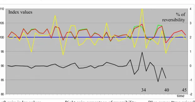
However, our methodology can be applied directly to real datasets, with no difficulties. Figure 2 presents the results of an estimation with T1 = 40 and T2 = 45. The green curve gives the

index values on [0,40], for the old dataset, the yellow curve gives the index values on [0,45], using only the new data T2\T1, and the red is for the completed sample. The black curve shows

the percentage of reversibility (Indt(45)/Indt(40) - 1) for t = 0,…,40. The sample of the new

data T2\T1 is smaller than the two others; thus its curve logically presents a higher volatility.

For the majority of the dates, the difference between the old index and the completed one is negligible; the black curve is close to zero. It is only in the last quarter of the interval [0,40] that the two curves can diverge (the spread can reach 1% with our simulated data). The direction of the variation is given by the new data. For instance, at t = 34 the index T2\T1 is at

110, whereas the old index is around 104. Consequently, the yellow curve brings the old value (104) to a higher level (105). As we can see, the reversibility phenomenon has a temporal pattern: it appears essentially for the nearest dates. This phenomenon is also documented by Clapham et al. (2006) and Deng and Quigley (2008). Unfortunately, from an investment point of view, these recent past values are in general the most important values. Therefore, it is crucial to elaborate a methodology able to indicate the level of reliability of the index values.

4.3. The simulation process

The Monte Carlo technique is well adapted to our problem. The simulation algorithm is presented in Figure 3 (in several points we could introduce some variations in the assumptions according to the needs of the modeling; here we present a basic version). From a repeat-sales sample on [0,T1] we calculate the associated index with R(T1) and Î(T1). These two quantities

are fixed during the entire process. The present is time T1, and we know that the two

(18)

We try to infer variations of the index when the estimation will be renewed at T2; in other

words, we would like to compare R(T1) and R(T2). Unfortunately, at point T1 the quantities

Î(T2), Î(T2\T1) and R(T2\T1) are unknown. The idea of the algorithm is to forecast these three

measures in order to solve the equation with unknown R(T2), and then to compare R(T1) and

R(T2). The first step consists of calibrating the exponential benchmark with the old data on

[0,T1]. More precisely, we are looking for the values of parameters K0 (constant flow on the

market) and α0 (resale speed) such that the total number of repeat-sales N and the total

quantity of information I is equal between the real dataset and the benchmark sample22_.

Mathematically speaking, we can estimate parameter α0 simply by working with quantity I/N,

which does not depend on K (numerical resolution). When α0 is known, we can calculate K0

with equation N = K T (1 – π ). Once the benchmark is calibrated, we assume that the arrival of the information on the interval [T1,T2] will occur according to the same rhythm as

previously. In this way we get an approximation23_Î

bench(T2\T1) for matrix Î(T2\T1). At the same

time, we also get an approximation for matrix Î(T2) adding Î(T1) and Îbench(T2\T1) (cf.

Proposition v). After the left side of Figure 3 devoted to informational matrixes, we now focus on the right side, dedicated to growth rate vectors, and try to infer vector R(T2\T1). R(T1) gives

the index evolution on interval [0,T1]. For the rest of interval [T1,T2], we complete it in a T2

-vector Rhyp = (R(T1), Rhyp(T1 ;T2)). Rhyp(T1 ;T2) is a scenario for the future of real estate prices.

In Simon (2007) we established that the vector R(T2\T1) is Gaussian. It is centered on the

growth rates of the theoretical index values,24_{and its variance-covariance matrix}25_{is σ} G²

Î(T2\T1)-1. Because of its unobservability at T1,we have to generate R(T2\T1) randomly as a

Gaussian vector

N

(Rhyp ; σG² Î(T2\T1)-1). The theoretical expectation (the true rates values) is

replaced here with the best estimator that we have on [0,T1] at T1, that is, R(T1), and we

complete it with the economic assumptions on [T1,T2] through vector Rhyp(T1 ;T2). For the

(19)

the process we know Î(T1), Î(T2\T1), Î(T2), R(T1), and R(T2\T1). The final step consists simply

of calculating vector R(T2) with the equation Î(T1)R(T1) + Î(T2\T1)R(T2\T1) = Î(T2)R(T2). Once

R(T2) is known, we can now calculate index values Intt(T2) on the interval [0,T1], and we can

measure the size of the reversibility phenomenon for each simulation of R(T2\T1). Repeatedly

running this procedure, we finally arrive at an empirical distribution of the spreads.

4.4. The theoretical law of reversibility in a simplified context

The Monte Carlo technique is interesting for the very complex situations in which closed formulas will be impossible to establish. For simple situations it is useful to deepen the mathematical analysis in order to get an idea of the dynamic of the revisions and to potentially model this phenomenon with a stochastic process. We start here with an initial repeat-sales sample ω0, associated with interval [0,T1]. In our model the benchmark is calibrated on this

dataset and, using the corresponding parameters, we get an estimation for matrix Î(T2\T1). The

quantities Î(T1), R(T1), Îbench(T2\T1), and Î(T2) are fixed and we just have one random source,

which is R(T2\T1). We also assume that vector Rhyp(T1 ;T2) is constant. Under these

assumptions and with the formula R(T2) = [Î(T2)]-1 [Î(T1)R(T1)+Îbench(T2\T1)R(T2\T1)], we can demonstrate that vector R(T2) is Gaussian and we have:

E[R(T2)] = R(T1) + [Î(T2)-1 Îbench(T2\T1)]Rhyp(T1;T2) V [R(T2)] = σG² [Î(T2)-1Îbench(T2\T1)][Î(T2)]-1 (6)

Matrix Îbench(T2\T1) represents new information, Î(T2), the total information. Consequently,

product Î(T2)-1 Îbench(T2\T1), which appears in these two formulas, can be interpreted as the

(vectorial) proportion of the new information contained in the total. The first formula simply asserts that the expectation of R(T2) is equal to the old and constant vector R(T1), plus a

quantity that represents the influence of the economic hypotheses Rhyp(T1;T2) on [T1,T2]. This

influence of Rhyp(T1;T2) is weighted by [Î(T2)]-1 Îbench(T2\T1); a relative measure of the

informational weight of the new data. Regarding the variance formula, we have to compare it with the formula26_{V [R(T}

(20)

the estimation for the index on [0,T2] directly with the entire dataset, without doing a halfway

estimation at T1. In a reversibility situation we already know a part of the total sample;

therefore the resulting index is less volatile. What is expressed with the second formula is simply that the attenuation coefficient for the volatility is nothing other than [Î(T2)]-1

Îbench(T2\T1), once more. Now, if we decide that on [T1,T2] real estate growth is null, in other

words, Rhyp(T1;T2) = 0, we can demonstrate27 the following result:

Reversibility law

For t = 1,…,T1 the ratio Indt(T2) / Indt(T1) is log-normally distributed:

LN

(0; v(t))

v(t) is the tth_{diagonal element of the matrix}28_σ

G²A(T2)

[

[Î(T2)]-1Îbench(T2\T1)

]

[ Î(T2)]-1 [A(T2)]’

The reversibility percentage29_{for date t is a random variable that we can write 100(Y} t – 1),

with Yt ~

LN

(0; v(t)). Figure 4 represents the theoretical deciles, anticipated at T1, using

sample ω0 on [0,T1]. The black curve gives the observed reversibility for this specific sample

when the horizon is extended from T1 to T2. As we can see, the theoretical curves are a good

approximation of the empirical one. The magnitude of the potential revisions is small and approximately constant for the left side of the interval. But on the right side, things are different. Near T1 the fluctuations are potentially more pronounced, as evidenced by the

divergence of the theoretical curves in Figure 4. With the methodology developed in this paragraph, it now becomes possible to anticipate and to quantify reversibility effects in a reliable way.

4.5. Comments

In the above algorithm, randomness appears with simulation of the Gaussian vector30

R(T2\T1). However, if we are interesting in deepening the simulation, we could introduce two

additional random sources: for vector Rhyp(T1 ;T2) and for the couple (K, α). Indeed, in order to

estimate the expectation of vector R(T2\T1), we completed vector R(T1) with Rhyp(T1 ;T2). This

(21)

as the future is uncertain, it could be reasonable to let these last coordinates fluctuate randomly, rather than restricting them to a single path. The second generalization concerns the couple (K, α). The first variable represents a constant level of liquidity in the market and the second the resale speed. With the calibration step on interval [0,T1] we found a mean couple

(K0,α0). However, we can think that for interval [T1,T2], market conditions might be slightly

different. To take this possibility into account we could randomly choose parameter K in an interval [K0 – ε ; K0 + ε] and α0 in [α0 – ε’ ; α0 + ε’], for each Monte-Carlo simulation. We

could even go further with this methodology, considering that the rhythm of transactions depends on the economic context and especially on future real estate prices. Here, we should first calibrate a proportional hazard model on [0,T1], like the one developed by Cheung, Yau,

and Hui (2004), for instance. Then, according to the scenario simulated on [T1,T2], the rhythm

of resales could be deduced. The last point we want to analyze in this paragraph is the direction of revisions. If we look at Figure 4, the probability of having a positive revision is equal to the probability of a negative one. But, from Clapp and Giaccotto (1999) we know that most of the time we have a downward revision, as is also documented by Clapham et al. (2006). Actually, it seems that there are two sides to the reversibility problem. The first corresponds to the decrease in variance of the estimators when more data become available, as shown in Figure 4; thanks to the methodology developed in this paper, we can easily have an idea of the magnitude of these revisions. The second aspect is a selectivity problem: the density of “flips” is higher near the right edge of interval [0,T1]. When the estimation horizon

is extended to T2, the relative weights between the flips and the goods with a longer holding

period come back to a more normal level for the dates near T1. It would not be a problem if

the financial features (trend and volatility) were the same across all types of goods, however, we have some evidence to suggest that this is not true (Clapham et al. (2006): “This suggests systematic differences in the relative appreciation of those early

(22)

entrants to the sample compared to those that arrive later”). The simplest solution to avoid the revision problem would be to exclude all “flips” from the estimation sample; however, with this choice we would also remove some interesting information about market conditions. If we want to estimate an index of the whole market, is it possible to deal with this problem using the formalism previously introduced? The answer is probably positive. For purposes of simplicity we are going to assume that the initial sample can be divided into two subsamples: flips (holding period < 2 years) and non-flips. For each subsample, we calculate for each elementary time interval [t,t+1] the quantities of relevant information: Iflips[t,t+1] and Inon-flips[t,t+1]. Near the right edge of the interval the ratio Iflips[t,t+1]/

Inon-flips[t,t+1] increases automatically. The idea of a correction would be to

remove just a portion of the flips from the global dataset in order to recover the same level for the ratio Iflips[t,t+1]/ Inon-flips[t,t+1] as the one we can

observe in the middle of the interval. After this initial correction of the selectivity problem we estimate the index on [0,T1]. Then, we apply the

methodology developed above to control for the revisions that do not depend on flips.

4.6. Derivatives and reversibility

In the last section of Clapham et al. (2006) several possibilities are investigated for the contract settlement of the derivatives. More precisely the issue is: when should cash flows be measured to give the best estimation of the true economic return realized between t and T, that is, Ln(IndexT/Indext)? Four choices are examined on a specific dataset (from the least to the

most effective):

(23)

2. Ln( IndT(T) ) – Ln( Indt(T) ) : current indexes

3. Ln( IndT(T+d) ) – Ln( Indt(t+d) ) : initial indexes delayed

4. Ln( IndT(T+d) ) – Ln( Indt(T+d) ) : current indexes delayed

We know that these four random variables are all centered on the true value: Ln(IndexT) –

Ln(Indext). The levels of reliability for these approximations are given by their respective

standard deviations. We establish formulas in appendix C for variances. As we can see, the formulas differ from that established in paragraph 4.4 with the reversibility law. How should we understand the difference? Actually, the reversibility law gives the conditional behavior for the revisions: we are at T1, we know value Indt(T1), and we want an idea of the variation of

this single index value when we re-estimate the index at T2. Here, in this paragraph, things are

different: we are looking at the absolute behavior of the revisions. In others words, we are at 0 and we want to forecast the error on the measure of the return, without knowing the index values at T1. Can we get back the ranking of Clapham et al. with our theoretical approach? If

we want to study this problem from a general point of view, we have to work with a “neutral” sample. We choose an exponential sample, assuming that K = 200, λ = 0.1, σG² = 0.001, and θ =

10 (conservative choice). Figure 5a gives the results for the no-delay situations, with three

choices for the resale date T (5, 30, and 45) and a purchase date t that varies between 0 and T-1. It appears clearly that the current choice is always better than the initial one. It is especially true for transactions with a purchase near the left edge of the interval. For repeat-sales with a purchase date in the middle or at the end of the estimation interval, a difference also exists, but in a smaller proportion. With Figure 5b we look at the delay effect for a transaction realized between t and T = 30. The three kinds of curves give the results for the no-delay situation, for a delay equal to 4 (four quarters), and for a delay equal to 8 (two years). When the measure of the return is realized one year later, the global quality of the approximation improves significantly compared with the no-delay choice. But when we extend the delay up

(24)

to two years, the additional improvement becomes lower (for instance, with the current choice and t = 10: no delay = 1.23%; delay one year = 1,11%; delay two years = 1,07%). From a cost/benefit point of view, this suggests that the optimal delay is maybe closer to one year than to two years. We also note that the no-delay current index is a bit problematic for repeat-sales with a purchase near T; as we can see, the quality of the measure deteriorates at the right of the interval. If we compare these results with the ones established in Clapham et al. (2006) we find the same ranking, except when we are dealing with delayed indexes. It seems that the current indexes are always better than the initial ones, according to this model. Moreover, we also bring to the fore the fact that the error strongly depends on the purchase date. If we want to go further in the study of the derivatives, the next step would be to choose a stochastic dynamic for the RSI in order to price the contingent claims. Unfortunately, things are rather complex because of the reversibility. If we consider the basic assumption for stochastic processes in finance (related to the concept of market efficiency), that is their Markovian31

behavior, a problem occurs. Is it really possible to describe the dynamic of the RSI with a single Markovian process? The answer is no. We can understand heuristically the problem in just rewriting the reversibility formula: Î(T2)R(T2) – Î(T1)R(T1) = Î(T2\T1)R(T2\T1). The left

side measures an increment between the present T1 and the future T2. If the Markovian

assumption is satisfied, this variation cannot depend on the dates before T1. But we know that

the right side Î(T2\T1)R(T2\T1), associated with new data arriving with the time extension, adds

information not only to [T1,T2] but also to interval [0,T1]. Consequently, RSI does not have a

Markovian behavior. What follows from this result is that we cannot use, at least directly, the usual stochastic dynamics (geometric Brownian motion, Ornstein-Uhlenbeck…) to price a contingent claim. A solution might be to describe the reversibility process itself with a dynamic related to the reversibility law, and then to model the RSI as a noisy asset, as in Childs et al. (2001, 2002a, 2002b). Using this approach, we could capture the price discovery

(25)

mechanism associated with the reversibility phenomenon. Even if the technical problems are important, the stakes are real and crucial for the finance industry. It is nothing less than the possibility of pricing the real estate derivatives written on the RSI.

5. Conclusion

By means of an informational reformulation of the RSI framework, we first established an intuitive and easy to handle formula for the reversibility phenomenon (cf. Appendix A for the example). Then, using an exponential benchmark for the resale decision and Monte-Carlo simulations, we developed a methodology for quantifying the size of the potential revisions, conditionally and unconditionally. In this way we answered the problem32_{mentioned in}

Clapham et al. (2006) for the repeat-sales index. For the moment, as we do not have a similar technique for the hedonic indexes, we cannot conclude that the RSI is not a suitable underlying for the derivatives contracts. Indeed, if its fluctuations are probably higher, they are nevertheless predictable, contrary to the hedonic approach. Regarding the best choice for settlement of the derivatives contracts, it seems that the current indexes with a delay equal to one year are the optimal choice. In this article we established that the reversibility phenomenon is not just a selectivity problem but also an inherent and intrinsic feature of the RSI. We probably cannot reduce the entire phenomenon to a single sample effect. The natural question for future researches is now to disentangle the two sources and to better understand their respective impacts.

(26)

References

Bailey, M.J., R.F. Muth, and H.O. Nourse. 1963. A Regression Method for Real Estate Price Index Construction. Journal of the American Statistical Association, 1962, 58.

Baroni, M., F. Barthélémy, and M. Mokrane. Physical Real Estate: A Paris Repeat Sales Residential Index. ESSEC Working paper DR 04007, ESSEC Research Center, ESSEC Business School, 2004.

Case, K.E, and R.J. Shiller. Prices of Single Family Homes since 1970: New Indexes for Four Cities. New England Economic Review, September/October 1987: 45-56.

Case, K.E, and R.J. Shiller. The Efficiency of the Market for Single-Family Homes. The American Economic Review, 1989, 79(1):125-137.

Chau, K.W., S.K. Wong, C.Y. Yiu, and H.F. Leung. Real Estate Price Indices in Hong-Kong. Journal of Real Estate Literature, 2005, 13(3): 337-356.

Cheung, S.L., K.W. Yau, and Y.V. Hui. The Effects of Attributes on the Repeat Sales Pattern of Residential Property in Hong-Kong. Journal of Real Estate Finance and Economics, 2004, 29(3):

321-Childs, P.D., S.H. Ott, and T.J. Riddiough. Valuation and Information Acquisition Policy for Claims Written on Noisy Real Assets. Financial Management, Summer 2001: 45-75.

Childs, P.D., S.H. Ott, and T.J. Riddiough. Optimal Valuation of Noisy Real Assets. Real Estate Economics, 2002a, 30(3): 385-414.

Childs, P.D., S.H. Ott, and T.J. Riddiough. Optimal Valuation of Claims on Noisy Real Assets: Theory and Application. Real Estate Economics, 2002b, 30(3): 415-443.

(27)

Clapham, E., P. Englund, J.M. Quigley, and C.L. Redfearn. Revisiting the Past and Settling the Score: Index Revision for House Price Derivatives. Real Estate Economics, 2006, 34(2): 275-302.

Clapp, J.M., and C. Giaccotto. Revisions in Repeat-Sales Price Indexes: Here Today, Gone Tomorrow?” Real Estate Economics, 1999, 27(1): 79-104.

Deng, Y., and J.M. Quigley. Index Revision, House Price Risk, and the Market for House Price Derivatives, 2008. Available on SSRN.

Gatzlaff, D., and D. Geltner. A Repeat-Sales Transaction-Based Index Of Commercial Property" A Study For The Real Estate Research Institute, 1998.

Hoesli, M., C. Giaccotto, and P. Favarger. Three New Real Estate Price Indices for Geneva, Switzerland. Journal of Real Estate Finance and Economics, 1997, 15(1): 93-109.

Meese, R.A., and N.E. Wallace. The Construction of Residential Housing Price Indices: A Comparison of Repeat-Sales, Hedonic-Regression and Hybrid Approaches. Journal of Real Estate Finance and Economics, 1997, 14: 51-73.

Simon, A. Information and Repeat-Sales. Working paper, available on SSRN, 2007.

Simon, A. Boundary Effects and Repeat-Sales. Working paper, available on SSRN, 2008.

Wang, F.T., and P.M. Zorn. Estimating House Price Growth with Repeat Sales Data: What’s the Aim of the Game?” Journal of Housing Economics, 1997, 6: 93-118.

(28)

Appendix A. Algebraic examples A1. Old index T1 on [0,2]

Old dataset

Time 0 1 2

House a pa,1 pa,2

House b pb,0 pb,1

House c pc,0 pc,2

Real distribution Informational distribution

ni,j 0 1 2 Li,j 0 1 2 0 1 1 0 1 0,5 1 1 1 1 2 2 1,5 0,5 2 0 0,5 1,5 0 2 Matrix Î Matrix η τ0_(T 1) = τ1(T1) = 2/1,5 ≈ 1,33

Purchase price in C(i,j) Resale price in C(i,j)

hp(i,j) 0 1 2 hf(i,j) 0 1 2

0 pb,0 pc,0 0 pb,1 pc,2

1 pa,1 1 pa,2

2 2

Mean purchase and resale prices in Sptt

Hp(0;T1) =

[

( pb,0 )1 ( pc,0 )0,5

]

1/ 1,5 Hp(1;T1) =

[

( pa,1 )1 ( pc,0 )0,5

]

1/ 1,5

We can understand these equations, for instance the first one, in the following way. The mean rate realized by the repeat-sales that are relevant for the interval [0,1] on their whole holding

(29)

periods, in other words ρ0(T1), depends on 75% of the first unitary index rate r0(T1), and on

25% of the second unitary index rate r1(T1). This set of transactions is more focused on the

first time-interval but not only because of the good c, bought at 0 and resold at 2. If we solve the system we get:

r0(T1) = 1,5 ρ0(T1) – 0,5 ρ1(T1)

r1(T1) = 1,5 ρ1(T1) – 0,5 ρ0(T1)

r0(T1) = 1/8 *

[

6 ln(pb,1/ pb,0) + 2 ln(pc,2/ pc,0) – 2 ln(pa,2/ pa,1)

A2. Index “new data” T2\T1 on [0,3]

New data

Time 0 1 2 3

House d pd,2 pd,3

House e pe,0 pe,3

ρ0(T2\T1) = 1/3 * [ ln(pe,3/ pe,0) ]

ρ1(T2\T1) = 1/3 * [ ln(pe,3/ pe,0) ]

ρ2(T2\T1) = 1/1,5*[(0,33/1,33) ln(pe,3/pe,0) + (1/1,33) ln(pd,3/pd,2)]

Estimation of the index: 0,33r0(T2\T1) + 0,33r1(T2\T1) + 0,33r2(T2\T1) = 1 ρ0(T2\T1)

0,33r0(T2\T1) + 0,33r1(T2\T1) + 0,33r2(T2\T1) = 1 ρ1(T2\T1)

0,33r0(T2\T1) + 0,33r1(T2\T1) + 1,33r2(T2\T1) = 2 ρ2(T2\T1)

A3. Completed index T2 on [0,3]

ρ0(T2) = 1/1,63*[(1/1,83)ln(pb,1/pb,0) + (0,5/1,83) ln(pc,2/pc,0) + (0,33/1,83) ln(pe,3/pe,0)]

ρ1(T2) = 1/1,63*[(1/1,83)ln(pa,2/pa,1) + (0,5/1,83) ln(pc,2/pc,0) + (0,33/1,83) ln(pe,3/pe,0)]

ρ2(T2) = 1/1,5 *[(0,33/1,33)ln(pe,3/pe,0) + (1/1,33) ln(pd,3/pd,2)]

Estimation of the index: 1,83r0(T2) + 0,83r1(T2) + 0,33r2(T2) = 3 ρ0(T2)

0,83r0(T2) + 1,83r1(T2) + 0,33r2(T2) = 3 ρ1(T2)

0,33r0(T2) + 0,33r1(T2) + 1,33r2(T2) = 2 ρ2(T2)

(30)

2 ρ2(T2) = 2 ρ2(T2)

And equivalently for vectors R:

1,83r0(T2)+0,83r1(T2)+0,33r2(T2) = [1,5r0(T1)+0,5r1(T1)]+[0,33r0(T2\T1)+0,33r1(T2\T1)+0,33r2(T2\T1)]

0,83r0(T2)+1,83r1(T2)+0,33r2(T2) = [0,5r0(T1)+1,5r1(T1)]+[0,33r0(T2\T1)+0,33r1(T2\T1)+0,33r2(T2\T1)]

0,33r0(T2)+0,33r1(T2)+1,33r2(T2) = 0 +[0,33r0(T2\T1)+0,33r1(T2\T1)+1,33r2(T2\T1)] Appendix B. Demonstration of the informational reversibility formulas

B1. Further details (estimation on [0,T1])

The number of repeat-sales in Splt_{is n}t_{= ∑}

i ≤ t < jni,j. For an element of

C

(i,j), the length of the

holding period is j – i. Using function G, we can define the G-mean33_ζt_{of these lengths in Spl}t

by ∑ i ≤ t < j ∑k’ G(j-i) = nt G(ζt). The first sum enumerates all the classes

C

(i,j) that belong to

Splt_{, the second, all the elements in each of these classes. Moreover, as G(j-i) measures the}

proportion of the time varying-noise Gk,t in the total noise for a repeat-sales of

C

(i,j), the

quantity G(ζt_{) can also be interpreted as the mean proportion of this Gaussian noise in the}

global one, for the entire subsample Splt_{. In the same spirit, we define the arithmetic average}

Ft_{of the holding frequencies 1/( j – i ), weighted by G( j – i ), in Spl}t_{: F}t₌

( nt_G(ζt_{) )}-1 _∑

i ≤ t < j∑k’G(j-i)*( 1 /(j-i) ) = It / (nt G(ζt)) . Its inverse τt = (Ft )-1 is then the

harmonic average34_{of holding periods j-i, weighted by G(j-i), in Spl}t_{. If at first the two}

averages ζt_{and τ}t_{appear to be two different concepts, in fact they are nothing of the sort. We}

always have, for each subsample Splt_{, ζ}t_{= τ}t_{(cf. Simon 2007 for more details).}

B2. Reversibility for I t_{and n}t

The table below exemplifies the extension of the horizon for the informational distribution. Two kinds of new repeat sales exist: those with a purchase before T1 and a resale after T1

(i < T1 < j ≤ T2), shown as solid lines, and those with a purchase and a resale between T1 and

(31)

the horizon is T1, are in light grey. And if the horizon becomes T2, the dark grey cells should

also be included in this set.

Informational distribution when the horizon is extended from T1 to T2

Solid lines: new repeat sales with a purchase before T1

and a resale after T1

(i<T1<j≤T2)

Dotted lines: new repeat sales with a purchase and a resale between T1

and T2 (T1≤ i < j ≤

T2)

For an interval [t,t+1], t < T1, the quantities of relevant information are It(T1) =

∑

i ≤ t < j ≤ T1Li,j for

the first horizon and It_(T

2) =

∑

i ≤ t < j ≤ T2 Li, j = It(T1) +

∑

i ≤ t < T1 < j ≤ T2Li,j for the second. The sum

with i ≤ t < T1 < j ≤ T2 corresponds to the additional information (dark grey). If we denote it

It_(T

2\T1), we simply get the relation It(T2) = It(T1) + It(T2\T1). Similarly, for the real equivalents

of It_(T

2), It(T1), and It(T2\T1), that is, nt(T2), nt(T1), and nt(T2\T1), we have exactly the same

kind of formula: nt_(T

2) = nt(T1) + nt(T2\T1). In what follows, the notation T2\T1 will refer to the

dataset of the new repeat sales that appear when the horizon is extended. B3. Reversibility for the mean prices Hp(t) and Hf(t)

We first calculate Hp(t) with the purchase prices for the two horizons:

[Hp(t,T1)]It(T1)=

Π

i ≤ t < j ≤T1( Πk’ pk’,i )1/ (Θ + (j – i )) [Hp(t,T2)]It(T2 )=

Π

i ≤ t < j ≤T2( Πk’ pk’,i )1/ (Θ + ( j – i ))

Therefore, we have:

hp(i,j)

)

Li,j =

Π

i ≤ t < T1 < j ≤ T2 ( Πk’ pk’,i )1/ (Θ + (j – i ))

0 1 … t t + 1 … T1 … T2 0 L0,1 … L0,t L0,t+1 … L0,T1 … L0,T2 1 … L1,t L1,t+1 … L1,T1 … L1,T2 ¦ … … … … t Lt,t+1 … Lt,T1 … Lt,T2 t + 1 … Lt+1,T1 … Lt+1,T2 ¦ … … … T1 … LT1,T2 ¦ … T2

(32)

For the interval [t,t+1], Hp(t, T2\T1) represents the mean purchase price for the new relevant

repeat sales. Thus, the reversibility formula is: [Hp(t,T2)]It(T2) = [Hp(t,T1)]It(T1)[Hp(t,T2\T1)]It(T2\T1).

As we can see, the new value Hp(t,T2) is the geometric average between the old value Hp(t,T1)

and a term that represents the new data: Hp(t,T2\T1). Their respective contributions are

Hf(t, T2 \ T1)

]

It( T2 \ T1)

B4. Reversibility for τt

We study in this section the link between the mean holding periods τt_(T

1) and τt(T2). We have:

It_(T

2\T1) =

∑

i ≤ t < T1 < j ≤ T2 Li,j =

∑

i ≤ t < T1 < j ≤ T2

∑

k’ G( j – i ) * ( 1 / ( j – i )). Thus, It(T2\T1) is almost

the arithmetic average of 1/(j-i) weighted by G(j-i). This formula lacks only the total mass of the weights, that is

∑

i ≤ t < T1 < j ≤ T2

∑

k’ G(j-i) = nt(T2\T1) G

(

ζ t(T2\T1)

)

, with ζt(T2\T1) the G-average

of the holding periods for the new repeat sales. Therefore, as in the basic situation, It_(T 2\T1) /

[

nt_(T

2\T1) G

(

ζ t(T2\T1)

)]

is a mean frequency Ft(T2\T1), and its inverse a mean harmonic

holding period τt_(T

2\T1) for the new repeat-sales. We can now establish the formal link

between τt_(T

[

nt_(T

2\T1)G(ζt(T2\T1))

]

/

τt(T2\T1). And, as we have nt(T2)G(ζt(T2)) = nt(T1)G(ζt(T1)) +

nt_(T

2\T1)G(ζt(T2\T1)), we can assert that τt(T2) is simply the harmonic weighted average of

τt_(T

1) and τt(T2\T1).

B5. Reversibility for ρt

B5a. Scalar formula for t < T1

For t < T1 we have35: ρt(T2) = [(1/τt(T1))*(lnHf(t,T1)-lnHp(t,T1))]*[ (It(T1)τt(T1)) /(It(T2)τt(T2))]

(33)

In the first square brackets we recognize ρt(T1). Moreover, we can easily prove that the third

brackets are also equal to [nt_(T

2\T1)G(ζ t(T2\T1))]-1 ∑ i ≤ t < T1 < j ≤ T2∑k’G(j-i)rk'(i,j). This expression is

simply the weighted mean of the mean rates rk'(i,j), for the new repeat sales. And, of course, we

denote it: ρt(T2\T1). Thus, the reversibility formula for ρt , t < T1, is:

ρt(T2) = [It(T1) / It(T2)][τt(T1) / τt(T2)]ρt(T1) + [It(T2\T1) / It(T2)][τt(T2\T1) / τt(T2)]ρt(T2\T1)

B5b. Vectorial formula

The above formula is valid for t < T1. However, the expressions that define It(T2\T1), τt(T2\T1),

ζ t_(T

2\T1), nt( T2 \ T1 ), and ρt(T2\T1) can be generalized for t ≥ T1. Indeed, in these expressions

the sums are for the classes C(i,j) such that i ≤ t < T1 < j ≤ T2 , that is the new repeat-sales

relevant for [t,t+1], with t < T1. Now, if we choose t ≥ T1, the relevant cells will be the ones

that satisfy36_{to i ≤ t < j ≤ T}

2. But what we get this way is not really new; it is just It(T2), τt(T2),

ζt_(T

2), nt( T2) and ρt(T2). For instance It(T2\T1) =

∑

i ≤ t < T1 < j ≤ T2Li,j gives for t ≥ T1:

∑

i ≤ t < j ≤ T2Li,j = It( T2). We can now write the reversibility formula for ρt in a more synthetic

manner. We regroup the values ρt(T2), for 0 ≤ t < T2, in a T2-vector P(T2) and the values ρt(T1),

for 0 ≤ t < T1, in a T1-vector P(T1). From vector P(T1), a T2-vector is created, adding to its end

T2-T1 zeros; it will be denoted in italics P(T1). The numbers ρt(T2\T1) are regrouped in a T2

-vector P(T2\T1). Its last T2-T1 coordinates are simply equal to ρt(T2). Thus, for t < T1 we have:

τt_(T

2) It(T2) ρt(T2) = It(T1) τt(T1) ρt(T1) + It(T2\T1) τt(T2\T1) ρt(T2\T1)

 nt_(T

2) G(ζt(T2)) ρt(T2) = nt(T1) G(ζt(T1)) ρt(T1) + nt(T2\T1) G(ζt(T2\T1)) ρt(T2\T1)

And for t ≥ T1:nt(T2) G(ζt(T2)) ρt(T2) = nt(T2\T1) G(ζt(T2\T1)) ρt(T2\T1)

The diagonal matrix η(T1) can be included in a T2-matrix, completing it with zeros, and

denoted in italics: η(T1). η(T2) is the usual T2-diagonal matrix. We denote η(T2\T1) the T2

-diagonal matrix that we get with n0_(T

2\T1)G(ζ0(T2\T1),…,nT2-1(T2\T1) G(ζT2-1(T2\T1)). We can

now write simultaneously these two kinds of equations (for t < T1 and for t ≥ T1):

(34)

B6. Reversibility for the informational matrix Î

For an interval [ti, tj] the relevant information is denoted I[ti, ti](T1) or I[ti, ti](T2), according to the

horizon. The associated informational matrixes are Î(T1) and Î(T2), dimension T1 and T2

respectively. A third matrix Î(T2\T1), dimension T2, is the link between Î(T1) and Î(T2). Its

values are calculated only with the new Li,j (cf. Table below), and for each interval [ti, tj] C

[0,T2] they represent the additional quantity of information.

Informational distribution for dataset T2\T1

0 1 … T1 T1 +1 … T2 0 0 … 0 L0,T1₊₁ … L0,T2 1 … 0 L1,T1₊₁ … L1,T2 ¦ ¦ ¦ … ¦ T1 LT1,T1₊₁ … LT1,T2 T1 +1 … L T1₊₁,T2 ¦ ¦ T2

We can write Î(T2\T1) with three submatrixes Îa(T2\T1), Îb(T2\T1), and Îc(T2\T1). Îa(T2\T1) and

Îc(T2\T1) are two square matrixes of dimension T1 and T2-T1, whereas Îb(T2\T1) is a T1*(T2-T1)

matrix and its transpose tÎb(T2\T1) a (T2-T1)*T1 matrix. Îa(T2\T1) is symmetric and its diagonal

elements correspond to the first column of Îb(T2\T1) ; from one of these diagonal elements,

the matrix values are the same on the right and below. The matrixes Îb(T2\T1) and Îc(T2\T1) are

simply extracted from Î(T2). Îa and Îc respectively represent the additional information for an

interval [ti,tj] C [0,T1] and [ti,tj] C [T1,T2]. Whereas Îb is for the intervals [ti,tj] C [0,T2] with ti

< T1 < tj. If we include now the matrix Î(T1) in a T2*T2 matrix, completing it with zeros and

denoting it in italics

Î

(T1), the reversibility formula for the informational matrix is simply:

Î(T2) =

Î

(T1) + Î(T2\T1).

Îa(T2\T1) Îb(T2\T1)

t _Î

b(T2\T1) Îc(T2\T1)

B7. Reversibility for the index

Î(T

2

\T

1