Quantitative chemical biosensing by bacterial chemotaxis in microfluidic chips: Chemotaxis-microfluidic biosensor

Supplementary Information to:

Quantitative chemical biosensing by bacterial chemotaxis in microfluidic chips

Clémence Roggo1_{, Cristian Picioreanu}2_{, Xavier Richard}3_{, Christian Mazza}3_{, Harald van Lintel}4 _and

Jan Roelof van der Meer1_*

1) Department of Fundamental Microbiology, University of Lausanne, 1015 Lausanne, Switzerland 2) Department of Biotechnology, Faculty of Applied Sciences, Delft University of Technology, 2629 HZ Delft, The Netherlands

3) Department of Mathematics, University of Fribourg, CH-1700 Fribourg, Switzerland

4) Microsystems Laboratory LMIS4, École Polytechnique de Lausanne (EPFL), Station 17, CH-1015 Lausanne, Switzerland

This supplementary information contains: - Supplementary Figures S1-S6

- Supplementary Tables S1, S2 - Metropolis script

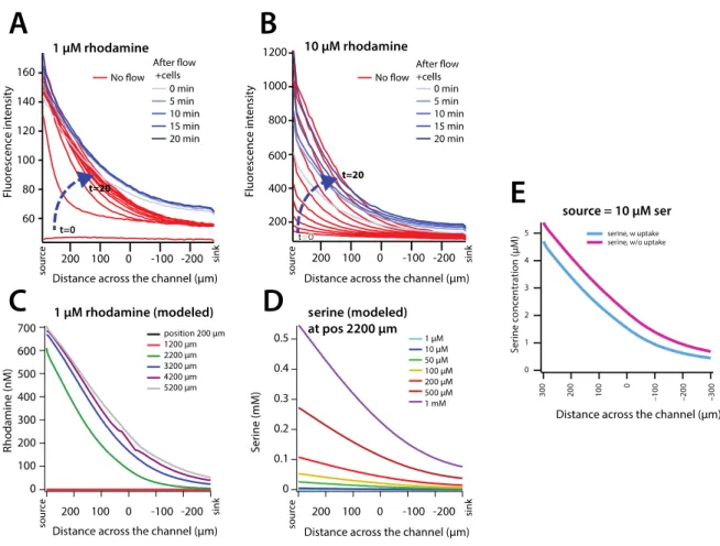
Figure S1. Gradient formation across the observation (middle) channel of the chip. Fluorescence profile formation across the channel without flow with (A) 1 µM or (B) 10 µM rhodamine in the source channel during 20 min (red lines, every 2 min), and after starting E. coli cell flow in the observation channel for another 20 min (blue lines, every 5 min). (C) Modeled rhodamine steady-state gradients at different transects along the observation channel. (D) Modeled serine gradients across the observation cell channel at position 2200 µm for seven source concentrations, as indicated, at the flow conditions computed as in Figure 1C. (E) Modeled effect of serine metabolism of E. coli on the established gradient at 10 µM serine source concentration and position 2200 µm in the observation channel. Note that for ease of comparison to the chip design, the distance across the channel is represented from 300 to –300 µm.

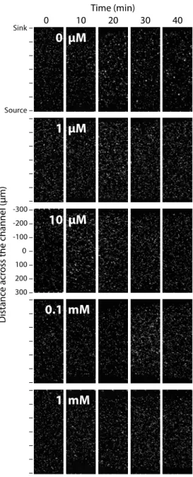
Figure S2: Non-chemotactic cell distribution of E. coli ∆fliC-mcherry toward serine. Images showing the distribution of ∆fliC-mcherry at the 2100-2200 µm location on the chip over time (0 - 40 min) as a function of the indicated serine concentration. Top is sink channel, bottom is source channel.

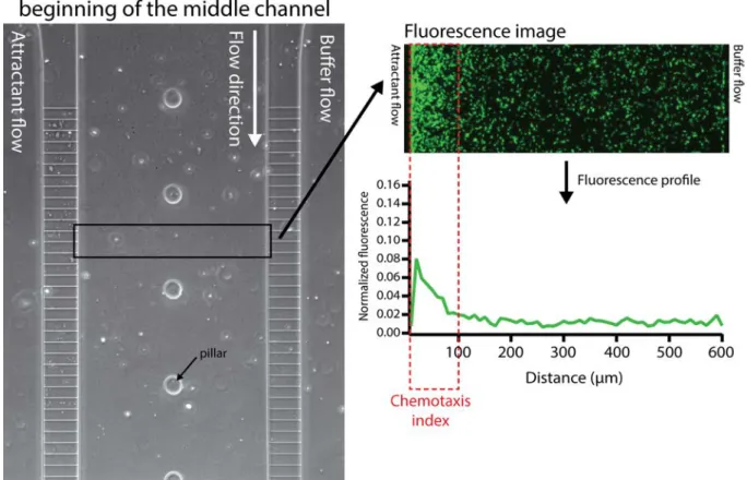
Figure S3: Chemotaxis index measurement setup. Chemotaxis response was quantified in a zone of 600 x 100 microns at a distance of 400 microns from the beginning of the filters. Fluorescence intensity profiles were extracted from the fluorescence images using ImageJ and normalized by the total fluorescence in the zone of measurement. The chemotaxis index was calculated as the proportion of fluorescence in the 100 µm segment closest to the source of attractant compared to the total fluorescence across the channel.

Figure S4: Microfluidic chip fabrication procedure. The fabrication procedure starts with a silicon wafer (1). A photolithography process produces a layer of resist at the filter position that protects this zone during the etching step (2). The etching results in the formation of the negative of the 650 nm high channels of the filters (3). A second step of photolithography produces the mold of thechannels with a resist layer of 14 microns high (4). This inverted mold is used multiple times to produce the PDMS chips, by pouring PDMS on it and let polymerize (5). Once polymerized, the PDMS is peeled off the inverted mold and, after punching holes for the inlets, is bonded to the glass slide by a plasma treatment (6).

Figure S5. (A) Model geometry, dimensions, domains and boundaries. Ω1: Source domain (fed with

chemoattractant solution), Ω2: Sink domain (fed with water), Ω3: Cells domain (fed with a suspension

of cells), Ω4 and Ω5: Filter domains (separate the cells from source and sink channels). Γi,1, Γi,2, Γi,3:

Inflows, Γo,1, Γo,2, Γo,3: Outflows. The geometry dimensions are listed in Table S1. (B) Finite element

Table S1. Parameters of the continuum steady-state model

Description Symbol Value Units Source

Geometry Height (z-direction) - channel - filter h 14 0.25 µm µm experimental Cell channel - width - length LY,3 LX,3 0.6 11.5 mm mm experimental Source and sink channels

- width - length LY,1 , LY,2 LX,1 , LX,2 1 9 mm mm experimental Inlet/outlet channels - width - length LX,i LY,i 0.26 2 mm mm experimental Filters - width - length LX,f LY,f 5 100 µm µm experimental

Filter spacing Lf 30 µm experimental

Flow

Water viscosity (at 20°C) µ 0.001 Pa s -

Water density ρ 1000 kg m–3 _-

Flow rate source/sink channels inlet

Fin,l 0.25 µL min–1 experimental

Flow rate cell channel inlet

Fin,m 0.003 µL min–1 experimental

Solutes Diffusion coefficienta) - rhodamine B - serine DS 3.6×10–10 8.9×10–10 m2 _s–1 _{(Culbertson et} al., 2002)

(Ma

Maximum serine uptake rate

vmax 338 nmol mmol–1

min–1 (Kayahara et al., 1992) Michaelis-Menten half-saturation coefficient Km 6 µmol L–1 (Kayahara et al., 1992) Cells

Basic motility coefficient DX 3×10–9 m2 s–1 estimated

Chemotaxis sensitivity coefficient

χ0 8×10–4 cm2 s–1 estimated after

(Chen et al., 1998)

a) corrected for 20 °C

b) To calculate the biomass in mM we use a typical elemental formula of E. coli cells of CH1.8O0.5N0.2

that corresponds to a molecular dry weight of 24.6 g/C-mol biomass. At an estimated individual E. coli cell weight of 300 fg and a starting suspension of 8·108 _{cells per mL, this corresponds to 10}

Table S2. Parameters, variables and functions used in the Metropolis model Description Symbol in script Symbol in main text

Value Units Source

Counter for simulation steps

s 0, 1, 2, ..., 1200 steps 1200

corresponds to 60 min Distance per time

step of simulation

d 20 µm Chosen

Grid width h Ly 600 µm Channel

width

Grid length l Lx 2500 µm Channel

length Cell simulation

window position

2000–2500 µm

Random angle r θ rand(0:360) degrees

Chemotactic sensitivity

ksi_0 ξ_ 1·105 _{- (Chen et al.,}

1998) Receptor-ligand dissociation constant c_dis KC 0.03 mM (Kalinin et al., 2009) Free parameter Gibbs-Boltzmann equation beta β -0.000013 - Fitting

Correction factor alpha α 0.4 - Fitting

Gradient Local serine concentration in y-direction for inlet concentration g(y) cS(p) mM 0 mM ser 0 mM Definition 0.001 mM ser -0.0006/(0.715*exp(-0.0056*y)+0.684)+0.00093 mM Fitting 0.01 mM ser -0.009/(1.027*exp(-0.005*y)+1)+0.0095 mM Fitting 0.1 mM ser -0.09/(1.34*exp(-0.005*y)+1.04)+0.092 mM Fitting 1 mM ser -0.9/(1.5*exp(-0.0054*y)+1.03)+0.9 mM Fitting Mean gradient Local serine starting c cS,0 mM

1 mM ser 0.279 mM Fitting Adaptation function a(t) _{1 (1 + 𝑒𝑒⁄} −𝑘𝑘∗( 𝑠𝑠_{100 −𝑠𝑠}0)₎ Logistic

function steepness k k mid-sigmoidal inflection point on simulation-axis s0 s0 0 mM ser 1 Definition 0.001 mM ser k=2.5; s0=0.01 - Fitting 0.01 mM ser k=2; s0=0.1 - Fitting 0.1 mM ser k=1.5; s0=2 - Fitting 1 mM ser k=1, s0=3 - Fitting

Metropolis script

function metropolis(x,y,g,d,c_dis,ksi_0,beta,alpha,a,c)

#x,y; starting position on the (x,y) grid within cell accumulation window position

#Number of simulation steps: 1200 (corresponding in the experiments to 60 min; so ~3 s equivalent to each simulation step). This function is called at each time step.

#Number of cells: 5000 #Number of simulations: 5

#sind(r): sinus in degrees of random angle #cosd(r): cosinus in degrees of random angle

#rand(): random number between 0 and 1 from a uniform distribution #h=600 (grid width) ## function H ## r = rand(0:360); Hx = ksi_0*(c_dis*c/(c+c_dis)^2)^alpha*(g(y)/c); Hy = ksi_0*(c_dis*c/(c+c_dis)^2)^alpha*(g(y+d*sind(r))/c); ## metropolis algorithm ## if sind(r)<=0 if y <= -d*sind(r) y = 0 x = x + d*cosd(r) else y = y + d*sind(r) x = x + d*cosd(r) end else if exp(-beta*a*(Hy-Hx)) >= rand() if y >= h - d*sind(r) y = h x = x + d*cosd(r) else y = y + d*sind(r) x = x + d*cosd(r) end end return [x,y] end

Supplementary references

Chen, K.C., Ford, R.M., and Cummings, P.T. (1998) Perturbation expansion of Alt's cell balance equations reduces to Segel's one-dimensional equations for shallow chemoattractant gradients. SIAM J Appl Math 59: 35-57.

Culbertson, C.T., Jacobson, S.C., and Ramsey, J.M. (2002) Diffusion coefficient measurements in microfluidic devices. Talanta 56: 365-373.

Kalinin, Y.V., Jiang, L., Tu, Y., and Wu, M. (2009) Logarithmic sensing in Escherichia coli bacterial chemotaxis. Biophys J 96: 2439-2448.

Kayahara, T., Thelen, P., Ogawa, W., Inaba, K., Tsuda, M., Goldberg, E.B., and Tsuchiya, T. (1992) Properties of recombinant cells capable of growing on serine without NhaB Na+/H+ antiporter in Escherichia coli. J Bacteriol 174: 7482-7485.

Ma, Y., Zhu, C., Ma, P., and Yu, K.T. (2005) Studies on the diffusion coefficients of amino acids in aqueous solutions. J Chem Eng Data 50: 1192-1196.