HAL Id: hal-03180730
https://hal.archives-ouvertes.fr/hal-03180730v4
Submitted on 26 May 2021
HAL is a multi-disciplinary open access
archive for the deposit and dissemination of
sci-entific research documents, whether they are
pub-lished or not. The documents may come from
teaching and research institutions in France or
L’archive ouverte pluridisciplinaire HAL, est
destinée au dépôt et à la diffusion de documents
scientifiques de niveau recherche, publiés ou non,
émanant des établissements d’enseignement et de
recherche français ou étrangers, des laboratoires
Faster One Block Quantifier Elimination for Regular
Polynomial Systems of Equations
Huu Phuoc Le, Mohab Safey El Din
To cite this version:
Huu Phuoc Le, Mohab Safey El Din. Faster One Block Quantifier Elimination for Regular
Polyno-mial Systems of Equations. International Symposium on Symbolic and Algebraic Computation 2021
(ISSAC ’21), Jul 2021, Saint Petersburg, Russia. �10.1145/3452143.3465546�. �hal-03180730v4�
FASTER
ONE
B
LOCK
QUANTIFIER
ELIMINATION FOR
REGULAR
P
OLYNOMIAL
SYSTEMS OF
EQUATIONS
Huu Phuoc Le Sorbonne Université, CNRS, Laboratoire d’Informatique de Paris 6, LIP6,
Équipe POLSYS
F-75252, Paris Cedex 05, France [email protected]
Mohab Safey El Din Sorbonne Université, CNRS, Laboratoire d’Informatique de Paris 6, LIP6,
Équipe POLSYS
F-75252, Paris Cedex 05, France [email protected]
May 26, 2021
A
BSTRACTQuantifier elimination over the reals is a central problem in computational real algebraic geometry, polynomial system solving and symbolic computation. Given a semi-algebraic formula (whose atoms are polynomial constraints) with quantifiers on some variables, it consists in computing a logically equivalent formula involving only unquantified variables. When there is no alternation of quantifiers, one has a one block quantifier elimination problem.
This paper studies a variant of the one block quantifier elimination in which we compute an almost equivalent formula of the input. We design a new probabilistic efficient algorithm for solving this variant when the input is a system of polynomial equations satisfying some regularity assumptions. When the input is generic, involves 𝑠 polynomials of degree bounded by 𝐷 with 𝑛 quantified variables and 𝑡 unquantified ones, we prove that this algorithm outputs semi-algebraic formulas of degree bounded by 𝒟 using 𝑂̃︀(︁(𝑛 − 𝑠 + 1) 8𝑡𝒟3𝑡+2(︀𝑡+𝒟
𝑡
)︀)︁
arithmetic operations in the ground field where 𝒟 = 2(𝑛 + 𝑠) 𝐷𝑠(𝐷 − 1)𝑛−𝑠+1(︀𝑛𝑠)︀. In practice, it allows us to solve quantifier elimination problems which are out of reach of the state-of-the-art (up to 8 variables). Keywords Quantifier elimination; Effective real algebraic geometry; Polynomial system solving
Huu Phuoc Le and Mohab Safey El Din are supported by the ANR grants ANR-18-CE33-0011 SESAME, and ANR-19-CE40-0018 DERERUMNATURA, the joint ANR-FWF ANR-19-CE48-0015 ECARP project and the European Union’s Horizon 2020 research and innovative training network program under the Marie Skłodowska-Curie grant agreement N° 813211 (POEMA).
1
Introduction
Problem statement. Let 𝑓 = (𝑓1, . . . , 𝑓𝑠) ⊂ Q[𝑦][𝑥] with 𝑥 = (𝑥1, . . . , 𝑥𝑛) and 𝑦 = (𝑦1, . . . , 𝑦𝑡). We aim at
solving the following quantifier elimination problem over the reals
This consists in computing a logically equivalent quantifier-free semi-algebraic formula Φ(𝑦), i.e. Φ is a finite disjunction of conjonctions of polynomial constraints in Q[𝑦] which is true if and only if the input quantified formula is true. The 𝑥 variables are called quantified variables and the 𝑦 variables are called parameters.
Let 𝜋 be the projection (𝑥, 𝑦) ↦→ 𝑦. Note that, geometrically, Φ describes the projection on the 𝑦-space of the real algebraic set 𝒱R⊂ R
𝑡
× R𝑛
defined by simultaneous vanishing of the 𝑓𝑖’s. In this paper, we focus on solving a
variant of the classical one block quantifier elimination, which computes a semi-algebraic formula which defines a dense subset of the interior of 𝜋(𝒱R).
Example 1. Consider the toy example 𝑥2+ 𝑦2 = 1. Its projection on the 𝑦 coordinate is described by the quantifier-free formula(𝑦 ≥ −1) ∧ (𝑦 ≤ 1) while for our variant quantifier elimination problem, an admissible output is (𝑦 > −1) ∧ (𝑦 < 1).
Except for proving theorems, this is sufficient for most of applications of quantifier elimination in engineering sciences or computing sciences where either the output formula only needs to define a sufficiently large subset of the 𝜋(𝒱R) or is evaluated with parameters’s values which are subject to numerical noise.
Prior works. The real quantifier elimination is a fundamental problem in mathematical logic and computational real algebraic geometry. It naturally arises in many problems in diverse application areas. The works of Tarski and Seidenberg [39,32] imply that the projection of any semi-algebraic set is also semi-algebraic and give an algorithm, which is however not elementary recursive, to compute this projection. The Cylindrical Algebraic Decomposition (CAD) [8] is the first effective algorithm for this problem whose complexity is doubly exponential in the number of indeterminates [11]. Since then, there have been extensive researches on developing this domain. We can name the CAD variants with improved projections [24,19,25,6] or the partial CAD [9]. Following the idea of [17] that exploits the block structure, [28,3] introduced algorithms of only doubly exponential complexity in the order of quantifiers (number of blocks). For one-block quantifier elimination, the arithmetic complexity and the degree of polynomials in the output of these algorithms are of order 𝑠𝑛+1𝐷𝑂(𝑛𝑡)where 𝐷 is the bound on the degree of input polynomials (see [4, Algo 14.6]). However, obtaining efficient implementations of these algorithms remains challenging. We also cite here some other works in real quantifier elimination [41,38,40,7,36] and applications to other fields [23,1,37].
In spite of this tremendous progress, many important applications stay out of reach of the state-of-the-art of the classic quantifier elimination. This motivates the researches on its variants. Generic quantifier elimination, in which the input and output formulas are equivalent for only almost every parameter, is studied in [12,33]. A practically efficient algorithm is presented in [20,21] for the same problem but under some assumptions on the input. The variant studied in this paper is a particular instance of the one in [20,21].
Main results. In this paper, we consider the input 𝑓 = (𝑓1, . . . , 𝑓𝑠) satisfying the assumptions below.
AssumptionA.
• The ideal of Q[𝑥, 𝑦] generated by 𝑓 is radical.
• The algebraic set 𝒱 ⊂ C𝑡+𝑛of𝑓 is equi-dimensional of dimension 𝑑 + 𝑡. Its singular locus has dimension
at most𝑡 − 1.
AssumptionB. The Zariski closure 𝜋(𝒱) of 𝜋(𝒱) is the whole parameter space C𝑡and𝜋(𝒱
R) is not of zero-measure
in R𝑡.
The first result of the paper is a new probabilistic algorithm for solving the aforementioned variant of the quantifier elimination on such an input 𝑓 . Our algorithm applies the algorithm of [30] to the system 𝑓 considering Q(𝑦) as the based field. This allows to reduce our problem to zero-dimensional polynomial systems in Q(𝑦)[𝑥]. Next, we compute semi-algebraic formulas that describe approximate projections of these systems on the 𝑦-space through the algorithm of [22]. This algorithm relies on a parametric variant of Hermite matrices for real root counting [27,18]. A similar outline is also presented in [40,13], in which the author computes an expensive comprehensive Gröbner bases [42] to analyze all cases before applying the real root counting algorithm of [27]. The relaxation of the output allows us to replace this exhaustive computation by the real root finding algorithm of [30].
Our second goal is to analyze the complexity of this new algorithm. For generic inputs, we bound the degree of the outputs and establish an arithmetic complexity which depends on this bound. The precise notion of genericity is as follows.
Let C[𝑥, 𝑦]≤𝐷= {𝑝 ∈ C[𝑥, 𝑦] | deg(𝑝) ≤ 𝐷}. A property 𝑃 is said to be generic over C[𝑥, 𝑦]𝑠𝐷if and only
if there exists a non-empty Zariski open subsetP ⊂ C[𝑥, 𝑦]𝑠
Our complexity result is then stated below. The notation 𝑂̃︀(𝑔) means 𝑂(𝑔 log
𝜅
(𝑔)) for some 𝜅 > 0. Theorem 1. Let 𝒟 = 2(𝑛 + 𝑠) 𝐷𝑠(𝐷 − 1)𝑛−𝑠+1(︀𝑛𝑠)︀. There exists a non-empty Zariski open subsetF of C[𝑥, 𝑦]𝑠≤𝐷
and a probabilistic algorithm such that, for every𝑓 ∈F , this algorithm, in case of success, computes a semi-algebraic formulaΦ defining a dense subset of the interior of 𝜋(𝑉 (𝑓 ) ∩ R𝑡+𝑛) within
𝑂̃︀(︀(𝑛 − 𝑠 + 1) 8𝑡𝒟3𝑡+2(︀𝑡+𝒟 𝑡
)︀)︀
arithmetic operations in Q and Φ involves only polynomials in Q[𝑦] of degree at most 𝒟.
Even though our complexity result has the same order as the one of [4, Algo 14.6], we obtain explicitly the degree bounds on the output formulas and the constant in the 𝑂 notation in the exponent.
On the practical aspect, our implementation in MAPLEof this algorithm outperforms real quantifier elimination functions in MAPLEand MATHEMATICA. It allows us to solve examples, both generic and non-generic, that are out of reach of these softwares (up to 8 indeterminates). These timings are reported in Section6.
Structure of the paper. In Section2, we start by recalling some basic notions. In Section3, we resume the algorithm for real root finding of [30]. Also in the same section, we prove some auxiliary results in order to apply this algorithm parametrically. Next, we dedicate Section4for the description of our algorithm for solving the targeted problem and proving its correctness. The complexity of this algorithm is analyzed in Section5. Finally, we report on some experimental results in Section6.
2
Preliminaries
Algebraic sets and critical points. Let F be a subfield of C and 𝐹 ⊂ F[𝑥1, . . . , 𝑥𝑛]. The algebraic subset
of C𝑛 at which the elements of 𝐹 vanish is denoted by 𝑉 (𝐹 ). For an algebraic set 𝒱 ⊂ C𝑛, we denote by 𝐼(𝒱) ⊂ C[𝑥1, . . . , 𝑥𝑛] the radical ideal associated to 𝒱. The singular locus of 𝒱 is denoted by sing(𝒱). Given any
subset 𝒮 of C𝑛, we denote by 𝒮 the Zariski closure of 𝒮, i.e., the smallest algebraic set containing 𝒮. An algebraic set
𝒱 is equi-dimensional if its irreducible components share the same dimension.
A map 𝜙 between two algebraic sets 𝒱 ⊂ C𝑛and 𝒲 ⊂ C𝑖is a polynomial map if there exist 𝜙1, . . . , 𝜙𝑖 ∈
C[𝑥1, . . . , 𝑥𝑛] such that 𝜙(𝜂) = (𝜙1(𝜂), . . . , 𝜙𝑖(𝜂)) for 𝜂 ∈ 𝒱. Let 𝒱 ⊂ C𝑛be an equi-dimensional algebraic
set. We denote by crit(𝜙, 𝒱) the set of critical points of the restriction of 𝜙 to the non-singular locus of 𝒱. If 𝑐 is the codimension of 𝒱 and (𝑓1, . . . , 𝑓𝑠) generates the ideal 𝐼(𝒱), the subset of 𝒱 at which the Jacobian matrix
jac(𝑓1, . . . , 𝑓𝑠, 𝜙1, . . . , 𝜙𝑖) of (𝑓1, . . . , 𝑓𝑠, 𝜙1, . . . , 𝜙𝑖) has rank less than or equal to 𝑐 is the union of crit(𝜙, 𝒱) and
sing(𝒱) (see, e.g., [31, Subsection 3.1]).
Gröbner bases and zero-dimensional ideals. Let F be a field and F be its algebraic closure. We fix an
admissible monomial order ≻ (see [10, Sec. 2.2]) over F[𝑥] where 𝑥 = (𝑥1, . . . , 𝑥𝑛). For 𝑝 ∈ F[𝑥], the leading
monomial of 𝑝 with respect to ≻ is denoted by lm≻(𝑝).
A Gröbner basis 𝐺 of an ideal 𝐼 ⊂ F[𝑥] w.r.t. the order ≻ is a finite generating set of 𝐼 such that the set of leading monomials {lm≻(𝑔) | 𝑔 ∈ 𝐺} generates ⟨lm≻(𝑝) | 𝑝 ∈ 𝐼⟩. For 𝑝 ∈ F[𝑥], the remainder of the division of 𝑝
by 𝐺 using the order ≻ is uniquely defined and is called the normal form of 𝑝 w.r.t. 𝐺. A polynomial 𝑝 is reduced by 𝐺 if 𝑝 equals to its normal form w.r.t. 𝐺.
An ideal 𝐼 is said to be zero-dimensional if the algebraic set 𝑉 (𝐼) ⊂ F𝑛is finite and non-empty. When this holds, by [10, Sec. 5.3, Theorem 6], the quotient ring F[𝑥]/𝐼 is a F-vector space of finite dimension. The dimension of this vector space is also called the algebraic degree of 𝐼; it coincides with the number of points of 𝑉 (𝐼) counted with multiplicities [4, Sec. 4.5]. For any Gröbner basis of 𝐼, the set of monomials in 𝑥 which are irreducible by 𝐺 forms a monomial basis, denoted by 𝐵, of this vector space. For 𝑝 ∈ F[𝑥], the normal form of 𝑝 by 𝐺 can be interpreted as its image in F[𝑥]/𝐼 and is a F-linear combination of elements of 𝐵.
Properness & Noether normalization. A map 𝜙 : 𝑉 ↦→ C𝑖is proper at 𝛽 ∈ C𝑖if there exists a neighborhood 𝒪 of 𝛽 such that 𝜙−1(𝒪) is compact, where 𝒪 denotes the closure of 𝒪 in the Euclidean topology. If 𝜙 is proper everywhere on its image, we say that the map 𝜙 is proper. The properness is strongly related to the following notion of Noether normalization.
Let F be a field and 𝐼 be an ideal of F[𝑥1, . . . , 𝑥𝑛]. The variables (𝑥𝑖+1, . . . , 𝑥𝑛) are in Noether position w.r.t.
𝐼 if their canonical images in the quotient algebra F[𝑥1, . . . , 𝑥𝑛]/𝐼 are algebraic integers over F[𝑥1, . . . , 𝑥𝑖] and
F[𝑥1, . . . , 𝑥𝑖] ∩ 𝐼 = ⟨0⟩. Once F = C and the variables (𝑥𝑖+1, . . . , 𝑥𝑛) is in Noether position w.r.t. 𝐼, the projection
of 𝑉 (𝐼) on (𝑥1, . . . , 𝑥𝑖) is proper.
Change of variables. Given a field F, we denote by GL(𝑛, F) the set of invertible matrices of size 𝑛 × 𝑛 with entries in F. Let 𝑝 ∈ F[𝑥] be a polynomial. For any 𝐴 ∈ GL(𝑛, F), we denote by 𝑝𝐴the polynomial 𝑝(𝐴 · 𝑥) ∈ F[𝑥]. For any algebraic set 𝑉 ⊂ F𝑛, 𝑉𝐴denotes the algebraic set {𝐴−1· 𝑥 | 𝑥 ∈ 𝑉 }.
For two blocks of indeterminates 𝑥 and 𝑦, we consider frequently the matrices that act only on the variables 𝑥 and leave 𝑦 invariant. Those matrices form a subset denoted by GL(𝑛, 𝑡, F) of GL(𝑛 + 𝑡, F).
3
Algorithm for real root finding
3.1 The 𝑆2algorithm
We recall the algorithm in [30], which we refer to as the 𝑆2algorithm, that computes at least one point per connected component of a smooth real algebraic set.
Let 𝑓 = (𝑓1, . . . , 𝑓𝑠) be a polynomial sequence in R[𝑥1, . . . , 𝑥𝑛]. For 1 ≤ 𝑖 ≤ 𝑑, let 𝜑𝑖be the projection
(𝑥1, . . . , 𝑥𝑛) → (𝑥1, . . . , 𝑥𝑖). When 𝑓 defines a smooth equi-dimensional algebraic set 𝒱 ⊂ C𝑛and generates a
radical ideal, one can build a polynomial system using appropriate minors of jac(𝑓 ) to define crit(𝜑𝑖, 𝒱). Note that
the critical loci are nested
crit(𝜑1, 𝒱) ⊂ crit(𝜑2, 𝒱) ⊂ · · · crit(𝜑𝑑, 𝒱) ⊂ crit(𝜑𝑑+1, 𝒱) = 𝒱.
Note also that in generic coordinates crit(𝜑𝑖, 𝒱) has expected dimension 𝑖 − 1. The algorithm in [30] then exploits
stronger properties of these critical loci under some genericity assumption on the coordinate system (which are satisfied through a generic linear change of coordinates).
Proposition 2. [30, Theorem 2] Assume that𝑓 defines a smooth equi-dimensional algebraic set and generates a radical ideal.
Then, there exists a non-empty Zariski open setA𝑓 ∈ GL(𝑛, C) such that for 𝐴 ∈ A𝑓the following holds:
• the restriction of 𝜑𝑖−1tocrit(𝜑𝑖, 𝒱𝐴) is proper;
• the set crit(𝜑𝑖, 𝒱𝐴) is either empty or of dimension 𝑖 − 1 for 1 ≤ 𝑖 ≤ 𝑑 + 1.
The first item in Proposition2implies the second one. The index in the notationA𝑓indicates that the non-empty
Zariski open set depends on 𝑓 . Algorithm 𝑆2considers fibers of the above critical loci with the convention 𝜋
0: 𝑥 → ∙.
Proposition2is the cornerstone of the 𝑆2algorithm which can be derived from the following one.
Proposition 3. [30, Theorem 2] Assume that𝑓 defines a smooth equi-dimensional algebraic set and generates a radical ideal.
For𝐴 ∈A𝑓∩ GL(𝑛, Q) as defined in Proposition2and𝛼 = (𝛼1, . . . , 𝛼𝑑) ∈ R𝑑, the union of the sets
crit(𝜑𝑖, 𝒱𝐴) ∩ 𝜑−1𝑖−1((𝛼1, . . . , 𝛼𝑖−1)), 1 ≤ 𝑖 ≤ 𝑑 + 1
is finite and meets all connected components of𝒱 ∩ R𝑛
. Example 4. Let 𝒱 be the smooth surface defined by 𝑥2
1− 𝑥22− 𝑥23= 1. The Jacobian matrix jac(𝑓 ) writes simply
(2𝑥1, −2𝑥2, −2𝑥3). It turns out that the identity matrix lies in the setA defined in Proposition2. Taking𝛼 = (0, 0),
we obtain 3 zero-dimensional systems:
• crit(𝜑1, 𝒱): {−2𝑥2, −2𝑥3, 𝑥21− 𝑥22− 𝑥23− 1},
• crit(𝜑2, 𝒱) ∩ 𝜑−11 (0): {−2𝑥3, 𝑥12− 𝑥22− 𝑥23− 1, 𝑥1},
• 𝒱 ∩ 𝜑−12 (0): {𝑥2
The first system admits two real solutions(1, 0, 0) and (−1, 0, 0). The other systems do not have any real solution. The two points(1, 0, 0) and (−1, 0, 0) intersect the two connected components of 𝒱.
Of course, on general examples, one would need to perform a randomly chosen linear change of variables but this example illustrates already how𝑆2works.
3.2 Parametric variant of 𝑆2
We present now a parametric variant of 𝑆2. We let 𝑓 = (𝑓1, . . . , 𝑓𝑠) ⊂ Q[𝑦][𝑥] where 𝑦 = (𝑦1, . . . , 𝑦𝑡) are
considered as parameters and 𝑥 = (𝑥1, . . . , 𝑥𝑛) are variables. The algebraic set defined by 𝑓 is denoted by
𝒱 ⊂ C𝑡
× C𝑛
. Let 𝜋 denote the projection (𝑥, 𝑦) ↦→ 𝑦 and 𝜋𝑖denote the projection (𝑦, 𝑥) ↦→ (𝑦, 𝑥1, . . . , 𝑥𝑖).
Considering Q(𝑦) as the ground field, the parametric variant of 𝑆2computes on the input 𝑓 a list of finite subsets of Q[𝑦][𝑥], each of which generates a zero-dimensional ideal of Q(𝑦)[𝑥]. These subsets are basically 𝑓𝐴∪ Δ𝐴
𝑖 ∪ {𝑥1− 𝛼1, . . . , 𝑥𝑖−1− 𝛼𝑖−1}, where (𝐴, 𝛼) is randomly chosen in GL(𝑛, 𝑡, Q) × Q𝑛and Δ𝐴𝑖 is the set
of all (𝑛 − 𝑑)-minors of the Jacobian matrix of 𝑓𝐴w.r.t. 𝑥𝑖, . . . , 𝑥𝑛.
The rest of this subsection is devoted to the auxiliary results that allow us to use the 𝑆2algorithm parametrically as above.
Lemma 5. When Assumptions (A) and (B) hold, there exists a non-empty Zariski open subsetB of C𝑡such that for every𝜂 ∈B, the specialization 𝑓(𝜂, ·) of 𝑓 at 𝜂 generates a radical equi-dimensional ideal whose algebraic set is either empty or has dimension𝑑.
Proof. Under Assumption (B), by the fiber dimension theorem [34, Theorem 1.25], there exists a non-empty Zariski open subsetB′of C𝑡such that 𝜋−1(𝜂) ∩ 𝒱 is an algebraic set of dimension 𝑑.
Let 𝒲 denote the set of points of 𝒱 at which the Jacobian matrix jac𝑥(𝑓 ) of 𝑓 w.r.t. 𝑥 has rank at most 𝑛 − 𝑑 − 1.
We note that 𝒲 = crit(𝜋, 𝒱) ∪ sing(𝒱). The algebraic version of Sard’s theorem [31, Proposition B2] implies that 𝜋(crit(𝜋, 𝒱)) is contained in a proper Zariski closed subset of C𝑡. On the other hand, as Assumptions (A) hold, the dimension of 𝜋 (sing(𝒱)) is less than 𝑡. Thus, it is also contained in a proper Zariski closed subset of C𝑡.
Hence, the Zariski closure of 𝜋(𝒲) is a proper Zariski closed subset of C𝑡. LetB be the intersection of the complement in C𝑡of this Zariski closure withB′. For 𝜂 ∈B, the set
{𝑥 ∈ C𝑛| 𝑓 (𝜂, 𝑥) = 0, rank jac𝑥(𝑓 )(𝜂) < 𝑛 − 𝑑}
is empty. Since the dimension of 𝜋−1(𝜂)∩𝒱 is 𝑑 and the Jacobian matrix jac𝑥(𝑓 )(𝜂, ·) of 𝑓 (𝜂, ·) w.r.t. the variables 𝑥 is of rank 𝑛 − 𝑑 for every (𝜂, 𝑥) ∈ 𝒱 ∩ 𝜋−1(𝜂), the ideal 𝑓 (𝜂, ·) is radical and defines a smooth and equi-dimensional set of dimension 𝑑 by Jacobian criterion [14, Theorem 16.19].
Lemma5shows that when specializing 𝑦 = (𝑦1, . . . , 𝑦𝑡) to a generic point 𝜂 ∈B ∩ R𝑡in 𝑓 , one obtains
𝑓 (𝜂, ·) satisfying the assumptions of Proposition2. One could then apply Algorithm 𝑆2to 𝑓 (𝜂, ·) to grab sample points in the real algebraic set it defines. However, proceeding this way would lead us to use a change of variables encoded by a matrix 𝐴 depending on 𝜂. The result below shows that choosing one generic change of variables will be valid for most of parameters’ values.
Proposition 6. Assume that Assumptions (A) and (B) hold. There exists a dense Zariski open subsetO of GL(𝑛, 𝑡, C) such that for every𝐴 ∈O ∩ GL(𝑛, 𝑡, Q) the following holds.
There exists a dense Zariski open subsetY𝐴of C𝑡such thatY𝐴is a subset of the Zariski open setB in Lemma5
and𝐴 lies in the Zariski open setA𝑓 (𝜂,.)defined in Proposition2for every𝜂 ∈Y𝐴.
Proof. Let C(𝑦) denote the algebraic closure of C(𝑦). We consider C(𝑦) as the coefficient field. The proof of [30, Theorem 1] is purely algebraic and then is valid over the based field C(𝑦). Hence, there exists a non-empty Zariski open subset ˜O of GL(𝑛, 𝑡, C(𝑦)) such that for 𝐴 ∈ ˜O ∩ GL(𝑛, 𝑡, Q), the variables (𝑥1, . . . , 𝑥𝑖−1) is in Noether
position w.r.t. the ideal in Q(𝑦)[𝑥] generated by 𝑓𝐴+ Δ𝐴𝑖 for 1 ≤ 𝑖 ≤ 𝑑 + 1 where Δ𝐴𝑖 is the set of maximal
minors of the truncated Jacobian matrix of jac(𝑓𝐴) with all the partial derivatives w.r.t. 𝑦 and 𝑥
𝑗for 1 ≤ 𝑗 ≤ 𝑖 being
This is equivalent to the following. For 1 ≤ 𝑖 ≤ 𝑑 + 1, 𝑖 ≤ 𝑗 ≤ 𝑛, there exist the polynomials 𝑝𝑖,𝑗 ∈
Q(𝑦)[𝑥1, . . . , 𝑥𝑖−1, 𝑥𝑗] such that each 𝑝𝑖,𝑗lies in the ideal of Q(𝑦)[𝑥] generated by 𝑓𝐴∪ Δ𝐴𝑖 and it is monic when
considering 𝑥𝑗as the only variable (with the coefficients in Q(𝑦)[𝑥1, . . . , 𝑥𝑖−1]).
The denominators of 𝑝𝑖,𝑗 are then polynomials in Q[𝑦]. We choose Y𝐴 to be the intersection of the
non-empty Zariski open setB defined in Lemma5and the non-empty Zariski open set defined by the non-vanishing of all the denominators appeared in the 𝑝𝑖,𝑗’s. Thus, for 𝜂 ̸∈Y𝐴, 𝑝𝑖,𝑗(𝜂, ·) ∈ Q[𝑥1, . . . , 𝑥𝑖−1, 𝑥𝑗] is monic in 𝑥𝑗.
Consequently, (𝑥𝑖, . . . , 𝑥𝑛) is in Noether position w.r.t. the ideal of C[𝑥] generated by 𝑓𝐴(𝜂, ·) ∪ Δ𝐴𝑖 (𝜂, ·). Finally,
takingO = ˜O ∩ GL(𝑛, 𝑡, C), the conclusion follows.
4
One-block QE algorithm
4.1 Description
In this subsection, we describe our algorithm for solving our variant of the quantifier elimination problem. The input is a polynomial sequence 𝑓 = (𝑓1, . . . , 𝑓𝑠) ⊂ Q[𝑥, 𝑦] satisfying Assumptions (A) and (B). Further, we denote by
𝑍(Ψ) the zero set of any semi-algebraic formula Ψ, i.e., 𝑍(Ψ) = {𝑦 ∈ R𝑡| Ψ(𝑦) is true}.
By Assumptions (A) and (B), the fiber dimension theorem [34, Theorem 1.25] implies that there exists a non-empty Zariski open subset of C𝑡such that 𝜋−1(𝜂) has dimension 𝑑. The idea is to apply the parametric variant of 𝑆2 with Q(𝑦) as a ground field.
More precisely, we start by picking randomly (𝐴, 𝛼) in GL(𝑛, 𝑡, Q) × Q𝑛and apply the change of variables 𝑥 ↦→ 𝐴 · 𝑥 to the input 𝑓 to obtain a new sequence 𝑓𝐴
. As 𝐴 acts only on 𝑥, 𝜋(𝑉 (𝑓𝐴) ∩ R𝑛+𝑡) = 𝜋(𝒱
R). Hence, a
quantifier-free formula that solves our problem for 𝑓𝐴is also a solution of the same problem for 𝑓 . Let jac𝑥(𝑓𝐴) be the Jacobian matrix of 𝑓𝐴w.r.t. the variables 𝑥 = (𝑥
1, . . . , 𝑥𝑛). We denote by 𝐽1, . . . , 𝐽𝑛
the columns of jac𝑥(𝑓 𝐴
) respectively. For 1 ≤ 𝑖 ≤ 𝑑, let 𝑊𝑖𝐴,𝛼be the union of 𝑓 𝐴
, all the (𝑛 − 𝑑)-minors of the matrix consisting of the columns 𝐽𝑖+1, . . . , 𝐽𝑛and {𝑥1− 𝛼1, . . . , 𝑥𝑖−1− 𝛼𝑖−1}. In particular, 𝑊𝑑+1𝐴,𝛼denotes
𝑓𝐴∪ {𝑥1− 𝛼1, . . . , 𝑥𝑑− 𝛼𝑑}.
We prove later in Lemma8that, for generic (𝐴, 𝛼), the ideals of Q(𝑦)[𝑥] generated by 𝑊𝑖𝐴,𝛼are radical and
zero-dimensional.
We now solve the quantifier elimination problem for each of the polynomial sets 𝑊𝑖𝐴,𝛼. For this step, we refer
to a subroutine called RealRootClassification that takes as input a polynomial sequence 𝐹 ⊂ Q[𝑦][𝑥] such that the ideal of Q(𝑦)[𝑥] generated by 𝐹 is radical and zero-dimensional and computes a quantifier-free formula Φ𝐹 in 𝑦
such that 𝑍(Φ𝐹) is dense in the interior of 𝜋(𝑉 (𝐹 ) ∩ R𝑛+𝑡). For this task, we refer to the algorithm of [22]. We will
explain the essential details of this subroutine later in Subsection4.2.
Calling the subroutine RealRootClassification on the inputs 𝑊𝑖𝐴,𝛼gives us the lists of semi-algebraic formulas Φ𝑖. Finally, we return Φ = ∨𝑑+1𝑖=1Φ𝑖as the output of our algorithm.
The pseudo-code below summarizes our algorithm, we introduce two additional subroutines:
• GenericDimension which takes the sequence 𝑓 and computes the dimension of the ideal generated by 𝑓 in Q(𝑦)[𝑥].
• (𝑛 − 𝑑) Minors which takes as input a matrix 𝑀 whose coefficients are in Q[𝑥, 𝑦] and computes all of its (𝑛 − 𝑑)-minors.
4.2 Real root classification
Now we explain the general ideas of the algorithm presented in [22] that is used in the RealRootClassification subroutine.
Let 𝐹 ⊂ Q[𝑦][𝑥] be a polynomial sequence such that the ideal ⟨𝐹 ⟩ generated by 𝐹 in Q(𝑦)[𝑥] is radical and zero-dimensional.
For such an input 𝐹 , RealRootClassification computes a semi-algebraic formula Φ𝐹 and a polynomial
Algorithm 1:One-block quantifier elimination
Input: 𝑓 ∈ Q[𝑦][𝑥] satisfying Assumptions (A) and (B). Output: A formula Φ s.t 𝑍(Φ) is dense in the interior of 𝜋(𝒱R).
1 Choose randomly (𝐴, 𝛼) ∈ GL(𝑛, Q) × Q𝑛 2 𝑓𝐴← 𝑓 (𝐴 · 𝑥) 3 [𝐽1, . . . , 𝐽𝑛] ← jac𝑥(𝑓 𝐴 ) 4 𝑑 ← GenericDimension(𝑓𝐴) 5 for 1 ≤ 𝑖 ≤ 𝑑 + 1 do 6 𝑊𝑖𝐴,𝛼← (𝑛 − 𝑑) Minors([𝐽𝑖+1, . . . , 𝐽𝑛]) ∪ {𝑓𝐴, 𝑥1− 𝛼1, . . . , 𝑥𝑖−1− 𝛼𝑖−1} 7 Φ𝑖← RealRootClassification(𝑊𝑖𝐴,𝛼) 8 return Φ ← ∨𝑑+1𝑖=1Φ𝑖 • 𝑍(Φ𝐹) ⊂ 𝜋(𝑉 (𝐹 ) ∩ R𝑛+𝑡), • 𝑍(Φ𝐹) ∖ 𝑉 (𝑤∞) = 𝜋(𝑉 (𝐹 ) ∩ R𝑛+𝑡) ∖ 𝑉 (𝑤∞).
The algorithm in [22] is based on constructing a symmetric matrix 𝐻𝐹 with entries in Q(𝑦) associated to 𝐹 . This
matrix is basically a parametric version of the classical Hermite matrix for the ideal ⟨𝐹 ⟩ (see, e.g., [4, Chap. 4]), which provides the number of distinct real/complex solutions of the system 𝐹 (𝜂, ·) through the signature/rank of the specialization of 𝐻𝐹 at 𝜂 [22, Corollary 17].
Let 𝐺𝐹be the reduced Gröbner basis of the ideal in Q[𝑥, 𝑦] generated by 𝐹 w.r.t. the grevlex(𝑥) ≻ grevlex(𝑦)
order. We consider the leading coefficients of the elements of 𝐺𝐹 in variables 𝑥 w.r.t. the grevlex(𝑥) order, which
are polynomials in Q[𝑦]. Then, 𝑤𝐹 is taken as the square-free part of the product of these leading coefficients.
The polynomial 𝑤𝐹 defines a proper algebraic subset of 𝑦-space over which the matrix 𝐻𝐹 does not have good
specialization property ([22, Proposition 16]).
Next, we choose randomly a matrix 𝑄 ∈ GL(𝛿, Q). As the entries of 𝐻𝐹lie in Q(𝑦), so do the leading principal
minors 𝑀1, . . . , 𝑀𝛿of 𝑄𝑇 · 𝐻𝐹· 𝑄. Let 𝑚1, . . . , 𝑚𝛿be the numerators of those minors, which are in Q[𝑦]. A
sufficiently generic matrix 𝑄 ensures that none of the 𝑚𝑖’s is identically zero, hence allowing us to determine the
signature of 𝐻𝐹according to the signs of the 𝑚𝑖’s. We then compute a finite set of points 𝐿 of Q𝑡that intersects
every connected component of the semi-algebraic set defined by ∧𝛿𝑖=1(𝑚𝑖̸= 0) ∧ (𝑤𝐹 ̸= 0). Over those connected
components, the polynomials 𝑚𝑖are sign-invariant. Since the signature of 𝐻𝐹(𝜂) can be deduced from the signs of
the 𝑚𝑖(𝜂), the number of real solutions of 𝐹 (𝜂, ·) is also invariant when 𝜂 varies in each connected component.
Let 𝐿0= {𝜂 ∈ 𝐿 | 𝐹 (𝜂, ·) admits at least one real solution} and
Φ𝐹 = (︁ ∨𝜂∈𝐿0 (︁ ∧𝛿 𝑖=1sign 𝑀𝑖= sign 𝑀𝑖(𝜂) )︁)︁ ∧ (𝑤𝐹 ̸= 0).
Then, 𝑤∞is taken as the product of the 𝑚𝑖’s and 𝑤𝐹. We return Φ𝐹, 𝑤∞as the output of RealRootClassification
for 𝐹 . The correctness of this algorithm is given in [22, Proposition 28]. In the pseudo-code below, we introduce the subroutines
• HermiteMatrix which takes as input a polynomial sequence 𝐹 ⊂ Q[𝑦][𝑥] such that the ideal ⟨𝐹 ⟩ ⊂ Q(𝑦)[𝑥] is zero-dimensional and computes the parametric Hermite matrix associated to 𝐹 w.r.t. the grevlex(𝑥) order.
The description of this subroutine is given in [22, Algo. 2].
• PrincipalMinors computes the leading principal minors of the matrix 𝑄𝑇· 𝐻𝐹· 𝑄.
• SamplePoints which takes as input a polynomial sequence 𝑚1, . . . , 𝑚𝛿, 𝑤𝐹 ∈ Q[𝑦] and computes
a finite set of points that intersects every connected component of the semi-algebraic set defined by ∧𝛿
𝑖=1𝑚𝑖̸= 0 ∧ 𝑤𝐹 ̸= 0.
We describe such a subroutine in [22, Sec. 3].
• Signature which evaluates the signature of a symmetric matrix of entries in Q. We end this subsection by an example to illustrate our algorithm.
Algorithm 2:RealRootClassification
Input: A polynomial sequence 𝐹 ⊂ Q[𝑦][𝑥] such that the ideal of Q(𝑦)[𝑥] generated by 𝐹 is radical and zero-dimensional.
Output: A formula Φ𝐹and a polynomial 𝑤∞∈ Q[𝑦]. 1 𝐻𝐹, 𝑤𝐹 ← HermiteMatrix(𝐹 )
2 Choose randomly 𝑄 ∈ GL(𝛿, Q) // 𝛿 is the size of 𝐻𝐹 3 (𝑀1, . . . , 𝑀𝛿) ← PrincipalMinors(𝑄𝑇· 𝐻𝐹 · 𝑄) 4 (𝑚1, . . . , 𝑚𝛿) ← Numerators(𝑀1, . . . , 𝑀𝛿) 5 𝐿 ← SamplePoints(︀(︀∧𝛿𝑖=1𝑚𝑖̸= 0)︀ ∧ 𝑤𝐹 ̸= 0)︀ 6 for 𝜂 ∈ 𝐿 do 7 if Signature (𝐻𝐹(𝜂)) ̸= 0 then 8 Φ𝐹 ← Φ𝐹∨(︀∧𝛿𝑖=1sign 𝑀𝑖= sign 𝑀𝑖(𝜂))︀ 9 Φ𝐹 ← Φ𝐹∧ (𝑤𝐹 ̸= 0) 10 𝑤∞← 𝑤𝐹 ·∏︀𝛿𝑖=1𝑚𝑖 11 return Φ𝐹, 𝑤∞
Example 7. We consider the polynomial 𝑓 = 𝑥21+ 𝑦1𝑥22+ 𝑦2𝑥2+ 𝑦3. LetΔ = 𝑦22− 4𝑦1𝑦3. The projection of
𝑉 (𝑓 ) ∩ R5on(𝑦1, 𝑦2, 𝑦3) is
(Δ ≥ 0 ∧ 𝑦1> 0) ∨ (𝑦1< 0) ∨ (𝑦1= 0 ∧ ((𝑦2̸= 0) ∨ (𝑦2= 0 ∧ 𝑦3≤ 0))) .
Applying the parametric variant of𝑆2for𝐴 = 𝐼3and𝛼 = (0, 0), we obtain 2 systems 𝑊1= {2𝑦1𝑥2+ 𝑦2, 𝑓 } and
𝑊2= {𝑓, 𝑥1}. Next, we call RealRootClassification on these systems, choosing 𝑄 = 𝐼2to simplify the calculation.
We obtain then𝑤1,∞= 𝑤2,∞= 𝑦1and the Hermite matrices:
𝐻1=(︂2 0 0 −2𝑦3+ 𝑦22/(2𝑦1) )︂ , 𝐻2= (︂ 2 −𝑦2/𝑦1 −𝑦2/𝑦1 (−2𝑦1𝑦3+ 𝑦22)/𝑦12 )︂ .
The sequences of leading principal minors are respectively[2, Δ/𝑦1] and [2, Δ/𝑦12]. We compute then 4 points
representing4 connected components of the semi-algebraic set defined by 𝑦1̸= 0 ∧ Δ ̸= 0:
(1, 1/8, 0), (−1, 1/8, 0), (1, 1/8, 1/128), (−1, 1/8, −1/128).
The matrix𝐻2 has non-zero signature over the first and second points, which both lead to the sign condition
Δ > 0 ∧ 𝑦21> 0. Thus, we have
Φ2= (Δ > 0 ∧ 𝑦12> 0) ∧ (𝑦1̸= 0).
For𝐻1, non-zero signatures are satisfied at the first and fourth points. Evaluating the sign ofΔ and 𝑦1at those points
gives
Φ1= ((Δ > 0 ∧ 𝑦1> 0) ∨ (Δ < 0 ∧ 𝑦1< 0)) ∧ (𝑦1̸= 0).
The final output is thereforeΦ = Φ1∨ Φ2, which is equivalent to
Φ = (Δ > 0 ∧ 𝑦1> 0) ∨ (Δ < 0 ∧ 𝑦1< 0) ∨ (Δ > 0 ∧ 𝑦1̸= 0)
= (Δ > 0 ∧ 𝑦1> 0) ∨ (Δ ̸= 0 ∧ 𝑦1< 0).
It is straight-forward to see that𝑍(Φ) is a dense subset of 𝜋(︀𝑉 (𝑓 ) ∩ R5)︀. 4.3 Correctness of Algorithm1
We start by proving that the polynomial sequences 𝑊𝑖𝐴,𝛼satisfy the assumptions required by RealRootClassification.
Lemma 8. Assume that Assumptions (A) and (B) hold. LetO be the Zariski open subset of GL(𝑛, 𝑡, C) defined in Proposition6and𝐴 ∈O ∩ GL(𝑛, 𝑡, Q). There exists a non-empty Zariski open subset X of C𝑑such that for 𝛼 ∈X ∩ Q𝑑
Proof. By Proposition6, the algebraic set defined by 𝑊𝑖𝐴,𝛼(𝜂, ·) is finite when 𝜂 varies over a non-empty Zariski
open subsetY𝐴of C𝑡. Thus, the ideal of Q(𝑦)[𝑥] generated by 𝑊𝑖𝐴,𝛼is zero-dimensional. Now we prove that the
ideal generated by 𝑊𝑖𝐴,𝛼is radical.
Let 𝑀1𝐴, . . . , 𝑀ℓ𝐴be the (𝑛 − 𝑑) minors of the Jacobian matrix 𝐽 associated to 𝑓 𝐴
when considering only the partial derivatives w.r.t. 𝑥𝑖+1, . . . , 𝑥𝑛. Recall that 𝑊𝑖𝐴,𝛼is the union of 𝑓
𝐴
with the 𝑀1𝐴, . . . , 𝑀ℓ𝐴 with
𝑥1− 𝛼1, . . . , 𝑥𝑖−1− 𝛼𝑖−1. Further, we denote by 𝑊′𝐴𝑖 ⊂ Q(𝑦)[𝑥] the ideal generated by 𝑓𝐴, 𝑀1𝐴, . . . , 𝑀ℓ𝐴.
The idea is to follow [31, Definitions 3.2 and 3.3] where charts and atlases are defined for algebraic sets defined by the vanishing of 𝑓𝐴and 𝑀1𝐴, . . . , 𝑀ℓ𝐴.
Let 𝑚 be a (𝑛 − 𝑑 − 1) minor of 𝐽 . Without loss of generality we assume that it is the upper left such minor and let 𝑀1𝐴, . . . , 𝑀𝑑−(𝑖−1)𝐴 be the (𝑛 − 𝑑) minors of 𝐽 obtained by completing 𝑚 with the 𝑛 − 𝑑-th line of 𝐽 and the
missing column. We denote by Q(𝑦)[𝑥]𝑚the localized ring where divisions by powers of 𝑚 are allowed.
By [31, Lemma B.12] there exists a non-empty Zariski open setO𝑚,𝑛−𝑑′ such that for 𝐴 ∈ GL(𝑛, 𝑡, C),
the localization of the ideal generated by 𝑓1𝐴, . . . , 𝑓𝑛−𝑑𝐴 , 𝑀1𝐴, . . . , 𝑀𝑑−(𝑖−1)𝐴 in the ring Q(𝑦)[𝑥]𝑚is radical and
coincides with the localization of 𝑊′𝐴𝑖 in Q(𝑦)[𝑥]𝑚. By [31, Prop. 3.4], there exists a non-empty Zariski open set
O′′
⊂ GL(𝑛, 𝑡, C) such that for 𝐴 ∈ O′′
, any irreducible component of the algebraic set defined by 𝑊′𝐴𝑖 contains
a point at which a (𝑛 − 𝑑 − 1) minor of 𝐽 does not vanish. This implies that any primary component 𝑊′𝐴𝑖 whose
associated algebraic set contains such a point is radical and then prime.
Now define Ω as the intersection ofO (defined in Proposition6), all non-empty Zariski open setsO𝑚,𝑘′ andO ′′
. Hence, we then deduce that 𝑊′𝐴𝑖 generates a radical ideal. It remains to prove that there exists a non-empty Zariski
open setX𝑖⊂ C𝑖−1such that for 𝛼 = (𝛼1, . . . , 𝛼𝑖−1) ∈X𝑖, ⟨𝑊′𝐴𝑖⟩ + ⟨𝑥1− 𝛼1, . . . , 𝑥𝑖−1− 𝛼𝑖−1⟩ is radical in
Q(𝑦)[𝑥]. Choosing 𝛼 outside the set of critical values of 𝜋𝑖restricted to the algebraic set defined by 𝑊′𝐴𝑖 in Q(𝑦) 𝑛
is enough. By Sard’s theorem, this set of critical values is contained in the vanishing set of a non-zero polynomial 𝜈 ∈ Q[𝑦][𝑥]. Now note that it suffices to define X𝑖as the complement of the vanishing set of the coefficients of 𝜈
when it is seen in Q[𝑥][𝑦] and X = ∩𝑑+1𝑖=1X𝑖.
We prove the correctness of Algorithm1in Proposition9below.
Proposition 9. Assume that Assumptions (A) and (B) hold. LetO ⊂ GL(𝑛, 𝑡, C) and X ⊂ C𝑑
be defined respectively in Proposition6and Lemma8. Then for𝐴 ∈ O ∩ GL(𝑛, 𝑡, Q) and 𝛼 ∈ X ∩ Q𝑑, the formulaΦ computed by Algorithm1defines a dense subset of the interior of𝜋(𝒱R).
Proof. By Lemma8, 𝑊𝑖𝐴,𝛼satisfies the assumptions of RealRootClassification. Thus, the calls of
RealRoot-Classification on 𝑊𝑖𝐴,𝛼are valid and return the formulas Φ𝑖and the polynomials 𝑤𝑖,∞. As 𝐴 acts only on 𝑥,
𝜋(𝒱R𝐴) = 𝜋(𝒱R). Thus,
𝑍(Φ𝑖) ⊂ 𝜋(𝑉 (𝑊𝑖𝐴,𝛼) ∩ R 𝑛+𝑡
) ⊂ 𝜋(𝒱R𝐴) = 𝜋(𝒱R).
Therefore, 𝑍(Φ) = ∪𝑑+1𝑖=1𝑍(Φ𝑖) ⊂ 𝜋(𝒱R).
By the description of Φ𝑖, for 1 ≤ 𝑖 ≤ 𝑑 + 1,
𝑍(Φ𝑖) ∖ 𝑉 (𝑤𝑖,∞) = 𝜋(𝑉 (𝑊𝑖𝐴,𝛼) ∩ R 𝑛+𝑡
) ∖ 𝑉 (𝑤𝑖,∞).
LetY𝐴be the non-empty Zariski open subset of C𝑡in Proposition6(Y𝐴depends on the matrix 𝐴). We denote
𝒲 = ∪𝑑+1𝑖=1𝑉 (𝑤𝑖,∞) ∪ (C𝑡∖Y𝐴).
We will show that, for 𝜂 ∈ 𝜋(𝒱R𝐴) ∖ 𝒲, 𝜂 ∈ 𝑍(Φ). Since 𝜂 ∈ 𝜋(𝒱R𝐴), 𝑉 (𝑓𝐴
(𝜂, ·)) ∩ R𝑛
is not empty. On the other hand, as 𝜂 ∈ 𝒴𝐴, 𝑓𝐴(𝜂, ·) generates a
radical equi-dimensional ideal whose algebraic set is either empty or smooth of dimension 𝑑. By Proposition3, 𝑉 (𝑓𝐴
(𝜂, ·)) ∩ R𝑛is not empty if and only if ∪𝑑+1 𝑖=1𝑉 (𝑊
𝐴,𝛼 𝑖 (𝜂) ∩ R
∪𝑑+1 𝑖=1𝜋(𝑉 (𝑊 𝐴,𝛼 𝑖 ) ∩ R 𝑛+𝑡 ) ∖ 𝒲. We have that ∪𝑑+1 𝑖=1𝜋(𝑉 (𝑊 𝐴,𝛼 𝑖 ) ∩ R 𝑛+𝑡 ) ∖ 𝒲 = ∪𝑑+1𝑖=1(𝜋(𝑉 (𝑊 𝐴,𝛼 𝑖 ) ∩ R 𝑛+𝑡 ) ∖ 𝒲) = ∪𝑑+1𝑖=1(𝑍(Φ𝑖) ∖ 𝒲) = (∪𝑑+1𝑖=1𝑍(Φ𝑖)) ∖ 𝒲.
Therefore, 𝑍(Φ) ∖ 𝒲 = 𝜋(𝒱R) ∖ 𝒲 and 𝜋(𝒱R) ∖ 𝑍(Φ) is of measure zero in R 𝑡
. By Assumption (B), we conclude that 𝑍(Φ) is a dense subset of the interior of 𝜋(𝒱R).
5
Complexity analysis
We now estimate the arithmetic complexity of Algorithm1once 𝐴 ∈O ∩ GL(𝑛, 𝑡, Q) and 𝛼 ∈ X ∩ Q𝑛as in
Proposition6are found from a random choice. In this section, the input 𝑓 forms a regular sequence of Q[𝑥, 𝑦] (then, 𝑠 = 𝑛 − 𝑑) satisfying Assumptions (A) and (B). As the calls to RealRootClassification on the systems 𝑊𝑖𝐴,𝛼are the
most costly parts of our algorithm, we focus on estimating their complexities. To this end, we introduce the following assumption.
AssumptionC. Let 𝐹 ⊂ Q[𝑥, 𝑦] and 𝐺 be the reduced Gröbner basis of 𝐹 w.r.t. the grevlex(𝑥) ≻ grevlex(𝑦)
order. Then𝐹 is said to satisfy Assumption (C) if and only if for any 𝑔 ∈ 𝐺, the total degree of 𝑔 in both 𝑥 and 𝑦 equals the degree of𝑔 w.r.t. only 𝑥.
In [22, Lemma 13], it is proven that, on an input 𝐹 satisfying Assumption (C), the polynomial 𝑤∞in
Real-RootClassification is simply 1 and the entries of the Hermite matrix 𝐻𝐹 are in Q[𝑦]. Therefore, the SamplePoints
subroutine is called on the sequence of leading principal minors of the parametric Hermite matrices. Again, with Assumption (C), the degree of these leading principal minors can be bounded (see [22, Lemma 32]). Therefore, one obtains the complexity bound for RealRootClassification for such 𝐹 .
Back to our problem, we will establish a degree bound for the polynomials given into SamplePoints. Some notations that will be used further are introduced below.
Let 𝐷 be a bound of the total degree of elements of 𝑓 . The zero-dimensional ideal of Q(𝑦)[𝑥] generated by 𝑊𝑖𝐴,𝛼is denoted by ⟨𝑊𝑖𝐴,𝛼⟩. The quotient ring Q(𝑦)[𝑥]/⟨𝑊𝐴,𝛼
𝑖 ⟩ is a finite dimensional Q(𝑦)-vector space. Let 𝐺𝑖
be the reduced Gröbner basis of the ideal of Q[𝑥, 𝑦] generated by 𝑊𝑖𝐴,𝛼w.r.t. grevlex(𝑥) ≻ grevlex(𝑦) and 𝐵𝑖be
the monomial basis of Q(𝑦)[𝑥]/⟨𝑊𝑖𝐴,𝛼⟩ constructed using 𝐺𝑖as in Section2. We begin with the following lemma.
Lemma 10. When Assumption (C) holds for 𝑊𝑖𝐴,𝛼, any leading principal minor of the matrix𝐻𝑖has degree bounded
by2∑︀
𝑏∈𝐵𝑖deg(𝑏).
Proof. The proof can be deduced from [22, Lemma 13, Proposition 31, Lemma 32]. It is mainly based on the control of degrees appearing in the normal form computation in Q(𝑦)[𝑥]/⟨𝑊𝑖𝐴,𝛼⟩.
It remains to estimate the sum∑︀
𝑏∈𝐵𝑖deg(𝑏). A bound is obtained by simply taking the product of the highest
degree appeared in 𝐵𝑖and its cardinality. As the Hilbert series of Q(𝑦)[𝑥]/⟨𝑊𝑖𝐴,𝛼⟩ when 𝑓 is a generic system are
known (see, e.g., [16,35]), explicit bounds of these quantities are easily obtained.
Lemma 11. Let 𝐵𝑖be defined as above. There exists a dense Zariski open subsetQ of C[𝑥, 𝑦]𝑠≤𝐷such that, for
𝑓 ∈Q, the following inequality holds for 1 ≤ 𝑖 ≤ 𝑑 + 1: ∑︀
𝑏∈𝐵𝑖deg𝑥(𝑏) ≤ (𝑛 + 𝑠 − 𝑖) 𝐷
𝑠
(𝐷 − 1)𝑛−𝑖−𝑠+2(︀𝑛−𝑖+1 𝑠 )︀.
Proof. By [26, Theorem 2.2], there exists a dense Zariski open subsetQ1,1⊂ C[𝑥, 𝑦]𝑠≤𝐷such that for 𝑓 ∈Q1,1,
the degree of ⟨𝑊1𝐴,𝛼⟩, which equals to the cardinality of 𝐵1, is bounded by
𝐷𝑠∑︀𝑛−𝑠 𝑘=0 (︀𝑘+𝑠−1 𝑠−1 )︀ (𝐷 − 1) 𝑘≤ 𝐷𝑠(𝐷 − 1)𝑛−𝑠(︀𝑛 𝑠)︀.
On the other hand, by [35, Corollary 3.2], there exists a dense Zariski open subsetQ1,2 ⊂ C[𝑥, 𝑦]𝑠≤𝐷such that
grevlex(𝑥), is bounded by (𝑛+𝑠−1)𝐷 −2𝑛+2. Thus, the highest degree in 𝐵1is bounded by (𝑛+𝑠−1)𝐷 −2𝑛+1.
Thus, letQ1=Q1,1∩Q1,2and, for 𝑓 ∈Q1, we obtain
∑︀
𝑏∈𝐵1deg(𝑏) ≤ (𝑛 + 𝑠 − 1) 𝐷
𝑠
(𝐷 − 1)𝑛−𝑠+1(︀𝑛 𝑠)︀.
For 1 ≤ 𝑖 ≤ 𝑑, the system 𝑊𝑖𝐴,𝛼can also be interpreted as the system defining the critical locus of the projection (𝑥𝑖, . . . , 𝑥𝑛) ↦→ 𝑥𝑖restricted to 𝑉(︀𝑓𝐴(𝛼1, . . . , 𝛼𝑖−1, 𝑥𝑖, . . . , 𝑥𝑛))︀. Therefore, by replacing 𝑛 by 𝑛 − 𝑖 + 1 in the
above bound, we deduce that, for 1 ≤ 𝑖 ≤ 𝑑, there exists a dense Zariski open subsetQ𝑖⊂ C[𝑥, 𝑦]𝑠≤𝐷such that
∑︀
𝑏∈𝐵𝑖deg(𝑏) ≤ (𝑛 + 𝑠 − 𝑖) 𝐷
𝑠(𝐷 − 1)𝑛−𝑖−𝑠+2(︀𝑛−𝑖+1 𝑠 )︀.
For 𝑖 = 𝑑 + 1, the cardinality of 𝐵𝑑+1is bounded by 𝐷𝑠and the highest degree in 𝐵𝑑+1is bounded by 𝑠(𝐷 − 1).
Thus, the bound holds for 𝑖 = 𝑑 + 1. TakingQ = ∩𝑑+1𝑖=1Q𝑖, we conclude the proof.
Further, 𝒟 denotes 2(𝑛 + 𝑠 − 1)𝐷𝑠(𝐷 − 1)𝑛−𝑠+1(︀𝑛
𝑠)︀. Now we show that Assumption (C) holds generically
then prove Theorem1.
Proposition 12. There exists a dense Zariski open subsetP ⊂ C[𝑥, 𝑦]𝑠
≤𝐷such that, for every𝑓 ∈P, there exists
a dense Zariski open subsetK𝑓 ⊂ GL(𝑛, 𝑡, C) × C𝑛such that for(𝐴, 𝛼) ∈K𝑓, Assumption(C) holds for every
system𝑊𝑖𝐴,𝛼.
Proof. Let 𝑦𝑡+1be a new variable andℎQ[𝑥, 𝑦, 𝑦𝑡+1]𝐷be the set of homogeneous polynomials in Q[𝑥, 𝑦, 𝑦𝑡+1]
of degree 𝐷. For 𝐹 ⊂ Q[𝑥, 𝑦], we denote byℎ𝐹 ⊂ Q[𝑥, 𝑦, 𝑦𝑡+1] the homogenization of 𝐹 w.r.t. all the variables
(𝑥, 𝑦), that meansℎ𝐹 = 𝑦deg(𝑝) 𝑡+1 · 𝐹 (︁ 𝑥1 𝑦𝑡+1, . . . , 𝑥𝑛 𝑦𝑡+1, 𝑦1 𝑦𝑡+1, . . . , 𝑦𝑡 𝑦𝑡+1 )︁
for each 𝑝 ∈ 𝐹 . Further, ⟨ℎ𝐹 ⟩ℎdenotes the
ideal of C[𝑥, 𝑦, 𝑦𝑡+1] generated byℎ𝐹 .
We consider the following property (C1): The leading terms appearing in the reduced Gröbner basis of ⟨ℎ𝐹 ⟩ℎ
w.r.t. grevlex(𝑥 ≻ 𝑦 ≻ 𝑦𝑡+1) do not involve any of the variables 𝑦1, . . . , 𝑦𝑡+1. By the proof of [22, Prop. 30], the
property (C1) implies Assumption (C).
Following the proof of [2, Prop. 7], if 𝑦𝑗+1 is not a zero-divisor of the quotient ring
C[𝑥, 𝑦, 𝑦𝑡+1]/⟨ℎ𝐹, 𝑦1, . . . , 𝑦𝑗⟩ℎfor every 0 ≤ 𝑗 ≤ 𝑡, then 𝐹 satisfies the property (C1). This property means
that (𝑦1, . . . , 𝑦𝑡+1) forms a regular sequence in the quotient ring C[𝑥, 𝑦, 𝑦𝑡+1]/⟨ℎ𝐹 ⟩ℎ. We name this property as
(C2).
From the proof of [35, Lemma 2.1, Lemma 2.2] and [14, Proposition 18.13], there exists a dense Zariski open subsetP1⊂ C[𝑥, 𝑦]𝑠≤𝐷such that for 𝑓 ∈P1, there exists a dense Zariski open subsetK𝑓 ,1⊂ GL(𝑛, 𝑡, C) × C𝑛
such that for (𝐴, 𝛼) ∈K𝑓 ,1, the quotient ring C[𝑥, 𝑦, 𝑦𝑡+1]/⟨ℎ𝑊1𝐴,𝛼⟩ℎis a Cohen-Macaulay ring of dimension
𝑡 + 1 and the ideal ⟨ℎ𝑊𝐴,𝛼
1 , 𝑦1, . . . , 𝑦𝑡+1⟩ℎhas dimension 0. By the unmixedness theorem [14, Corollary 18.14],
(𝑦1, . . . , 𝑦𝑡+1) is a regular sequence over C[𝑥, 𝑦, 𝑦𝑡+1]/⟨ℎ𝑊1𝐴,𝛼⟩ℎ. Thus, 𝑊1𝐴,𝛼satisfies the property (C2) and
Assumption (C) holds.
Similar for 2 ≤ 𝑖 ≤ 𝑑 + 1, we obtain dense Zariski subsetsP𝑖⊂ C[𝑥, 𝑦]𝑠≤𝐷andK𝑓 ,𝑖⊂ GL(𝑛, 𝑡, C) × C𝑛
for each 𝑓 ∈P𝑖. TakingP = ∩𝑑+1𝑖=1P𝑖, andK𝑓 = ∩𝑑+1𝑖=1K𝑓 ,𝑖, we conclude the proof.
Proof of Theorem1. It is well-known that Assumptions (A) and (B) are generic. Also, the set of regular sequences is dense in C[𝑥, 𝑦]𝑠≤𝐷. Thus, there exists a dense Zariski open subsetR ⊂ C[𝑥, 𝑦]𝑠≤𝐷such that for any 𝑓 ∈R,
𝑓 forms a regular sequence satisfying Assumptions (A) and (B). As 𝑉 (𝑓 ) has dimension 𝑑 + 𝑡 and 𝑓 forms a regular sequence in Q[𝑥, 𝑦], 𝑑 = 𝑛 − 𝑠. Algorithm1consists of (𝑑 + 1) calls to RealRootClassification on 𝑊𝑖𝐴,𝛼. LetP be the dense Zariski open set in Proposition12andQ = P ∩ R. Then, for 𝑓 ∈ Q, SamplePoints is called on a list of polynomials in Q[𝑦] of degree bounded by 𝒟. The number of principal minors is equal to the dimension of the quotient ring Q(𝑦)[𝑥]/⟨𝑊𝑖𝐴,𝛼⟩, which is also bounded by 𝒟. Applying [22, Theorem 2], each call
to RealRootClassification on 𝑊𝑖𝐴,𝛼costs at most 𝑂̃︀(︀8𝑡𝒟3𝑡+2(︀𝑡+𝒟
𝑡 )︀)︀ arithmetic operations in Q. In total, the
arithmetic complexity of Algorithm1is bounded by 𝑂̃︀(︀(𝑛 − 𝑠 + 1) 8𝑡𝒟3𝑡+2(︀𝑡+𝒟 𝑡 )︀)︀.
6
Experiments
We compare the practical behavior of Algorithm1with QuantifierElimination (MAPLE’s RegularChains) and Resolve (MATHEMATICA) on an Intel(R) Xeon(R) Gold 6244 3.60GHz machine of 754GB RAM. The timings are given in seconds (s.), minutes (m.) and hours (h.). The symbol ∞ means that the computation is stopped after 72 hours without getting the result. We use ourMAPLEimplementation for Hermite matrices, in which FGBpackage [15] is used for Gröbner bases computation. The computation of sample points is done by RAGLIB[29] which uses msolve [5] for polynomial system solving.
For RealRootClassification, we use the following notations:
• HM: timings of computing Hermite matrices and their minors. • SP: total timings of computing the sample points.
• SIZE: the largest size of the Hermite matrices.
• DEG: the highest degree appeared in the output formulas.
Start with random dense systems, we fix the total degree 𝐷 = 2 and run our algorithm for various (𝑡, 𝑛, 𝑠). In Table1, SamplePoints accounts for the major part of our timings. While our algorithm can tackle these examples, neither MAPLEnor MATHEMATICAfinish within 72h. The theoretical degree bound agrees with the practical observations. This agrees with our complexity result. On smaller problems, we observe that formulas computed byMAPLEandMATHEMATICAhave larger degrees than our output. Hence, these implementations, based on CAD, suffer from its doubly exponential complexity while our implementation takes advantage of the singly exponential complexity of our algorithm.
𝑡 𝑛 𝑠 HM SP SIZE DEG MAPLE MATHEMATICA
2 3 2 .2 s. 3 s. 8 24 ∞ ∞ 2 4 2 9 s. 1 m. 12 40 ∞ ∞ 2 5 2 2 m. 15 m. 16 56 ∞ ∞ 2 6 2 20 m. 2.5 h. 20 72 ∞ ∞ 2 7 2 1.5 h. 6 h. 24 88 ∞ ∞ 3 3 2 6 s. 1 m. 8 24 ∞ ∞ 3 4 2 5 m. 15 m. 12 40 ∞ ∞ 3 5 2 2 h. 5 h. 16 56 ∞ ∞ 3 6 2 8 h. 16 h. 20 72 ∞ ∞ 4 3 2 40 s. 30 m. 8 24 ∞ ∞ 4 4 2 6 h. 40 h. 12 40 ∞ ∞ 5 3 2 5 m. 14 h. 8 24 ∞ ∞
Table 1: Generic systems with 𝐷 = 2
Table2shows the timings for sparse systems. Each polynomial is generated with 𝐷 = 2 and has 2𝑛 terms. Even Assumption (C) is not satisfied, our algorithm still applies. Thanks to the sparsity, the size and degree of the matrices in our algorithm are smaller than in the dense cases. Thus, our algorithm runs faster here than in Table1while these examples are out of reach ofMAPLEandMATHEMATICA.
𝑡 𝑛 𝑠 HM SP SIZE DEG MAPLE MATHEMATICA
3 3 2 3 s. 37 s. 7 22 ∞ ∞ 3 4 2 2 m. 10 m. 9 34 ∞ ∞ 3 5 2 2 m. 10 m. 9 32 ∞ ∞ 4 3 2 20 s. 20 m. 7 22 ∞ ∞ 4 4 2 15 s. 18 m. 5 20 ∞ ∞
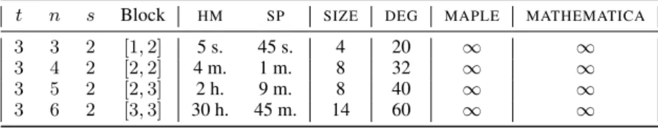
Table3gives the timings for structured systems. We separate the variables 𝑥 into blocks of total degree 1; [𝑖, 𝑛 − 𝑖] means that the degree in [𝑥1, . . . , 𝑥𝑖] and [𝑥𝑖+1, . . . , 𝑥𝑛] are respectively 1. Here, entries of the Hermite
matrices have non-trivial denominators with high degree. Computation those matrices takes the major part. However, our algorithm still outperforms the two other software.
𝑡 𝑛 𝑠 Block HM SP SIZE DEG MAPLE MATHEMATICA
3 3 2 [1, 2] 5 s. 45 s. 4 20 ∞ ∞ 3 4 2 [2, 2] 4 m. 1 m. 8 32 ∞ ∞ 3 5 2 [2, 3] 2 h. 9 m. 8 40 ∞ ∞ 3 6 2 [3, 3] 30 h. 45 m. 14 60 ∞ ∞
Table 3: Structured systems
References
[1] Hirokazu Anai and Volker Weispfenning. Reach set computations using real quantifier elimination. In Hybrid Systems: Computation and Control, pages 63–76. Springer Berlin Heidelberg, 2001.
[2] Magali Bardet, Jean-Charles Faugère, and Bruno Salvy. On the complexity of the F5 Gröbner basis algorithm. J. Symb. Comput., 70:49–70, 2015.
[3] Saugata Basu, Richard Pollack, and Marie-Françoise Roy. On the combinatorial and algebraic complexity of quantifier elimination. J. ACM, 43(6):1002–1045, November 1996.
[4] Saugata Basu, Richard Pollack, and Marie-Françoise Roy. Algorithms in Real Algebraic Geometry. Springer-Verlag, Berlin, Heidelberg, 2006.
[5] Jérémy Berthomieu, Christian Eder, and Mohab Safey El Din. msolve: A Library for Solving Polynomial Systems. Preprint, February 2021.
[6] Christopher W. Brown. Improved projection for Cylindrical Algebraic Decomposition. J. Symb. Comput., 32(5):447 – 465, 2001.
[7] Christopher W. Brown and Christian Gross. Efficient preprocessing methods for quantifier elimination. In Computer Algebra in Scientific Computing, pages 89–100, Berlin, Heidelberg, 2006. Springer Berlin Heidelberg. [8] George E. Collins. Quantifier elimination for real closed fields by cylindrical algebraic decomposition: a
synopsis. ACM SIGSAM Bulletin, 10(1):10–12, 1976.
[9] George E. Collins and Hoon Hong. Partial Cylindrical Algebraic Decomposition for quantifier elimination. J. Symb. Comput., 12(3):299 – 328, 1991.
[10] David A. Cox, John Little, and Donal O’Shea. Ideals, Varieties, and Algorithms: An Introduction to Computa-tional Algebraic Geometry and Commutative Algebra, (Undergraduate Texts in Mathematics). Springer-Verlag, Berlin, Heidelberg, 2007.
[11] James H. Davenport and Joos Heintz. Real quantifier elimination is doubly exponential. J. Symb. Comput., 5(1):29 – 35, 1988.
[12] Andreas Dolzmann, Thomas Sturm, and Volker Weispfenning. A new approach for automatic theorem proving in real geometry. J. Autom. Reason., 21(3):357–380, December 1998.
[13] Andreas Dolzomann and Lorenz A. Gilch. Generic hermitian quantifier elimination. In Bruno Buchberger and John Campbell, editors, Artificial Intelligence and Symbolic Computation, pages 80–93, Berlin, Heidelberg, 2004. Springer Berlin Heidelberg.
[14] David Eisenbud. Commutative Algebra: With a View Toward Algebraic Geometry. Graduate Texts in Mathematics. Springer, 1995.
[15] Jean-Charles Faugère. FGb: A Library for Computing Gröbner Bases. In Mathematical Software - ICMS 2010, volume 6327 of Lecture Notes in Computer Science, pages 84–87. Springer Berlin / Heidelberg, 2010. [16] Jean-Charles Faugère, Mohab Safey El Din, and Pierre-Jean Spaenlehauer. On the complexity of the generalized
minrank problem. J. Symb. Comput., 55:30 – 58, 2013.
[18] Charles Hermite. Sur le nombre des racines d’une équation algébrique comprises entre des limites données. extrait d’une lettre á m. borchardt. J. Reine Angew. Math., 52:39–51, 1856.
[19] Hoon Hong. An improvement of the projection operator in Cylindrical Algebraic Decomposition. In Proceedings of the International Symposium on Symbolic and Algebraic Computation, ISSAC ’90, page 261–264, New York, NY, USA, 1990. Association for Computing Machinery.
[20] Hoon Hong and Mohab Safey El Din. Variant real quantifier elimination: Algorithm and application. In Proceedings of the 2009 International Symposium on Symbolic and Algebraic Computation, ISSAC ’09, page 183–190, New York, NY, USA, 2009. Association for Computing Machinery.
[21] Hoon Hong and Mohab Safey El Din. Variant quantifier elimination. J. Symb. Comput., 47(7):883 – 901, 2012. International Symposium on Symbolic and Algebraic Computation (ISSAC 2009).
[22] Huu Phuoc Le and Mohab Safey El Din. Solving parametric systems of polynomial equations over the reals through Hermite matrices. Preprint, November 2020.
[23] Richard Liska and Stanly L. Steinberg. Applying Quantifier Elimination to Stability Analysis of Difference Schemes. The Computer Journal, 36(5):497–503, 01 1993.
[24] Scott McCallum. An improved projection operation for Cylindrical Algebraic Decomposition of three-dimensional space. J. Symb. Comput., 5:141 – 161, 1988.
[25] Scott McCallum. On projection in CAD-based quantifier elimination with equational constraint. In Proceedings of the 1999 International Symposium on Symbolic and Algebraic Computation, ISSAC ’99, page 145–149, New York, NY, USA, 1999. Association for Computing Machinery.
[26] Jiawang Nie and Kristian Ranestad. Algebraic degree of polynomial optimization. SIAM J. on Optimization, 20(1):485–502, April 2009.
[27] P. Pedersen, Marie-Françoise Roy, and Aviva Szpirglas. Counting real zeros in the multivariate case. In Frédéric Eyssette and André Galligo, editors, Computational Algebraic Geometry, pages 203–224, Boston, MA, 1993. Birkhäuser Boston.
[28] James Renegar. On the computational complexity and geometry of the first-order theory of the reals. Part III: Quantifier elimination. J. Symb. Comput., 13(3):329–352, March 1992.
[29] Mohab Safey El Din. Real alebraic geometry library, RAGlib (version 3.4), 2017.
[30] Mohab Safey El Din and Éric Schost. Polar varieties and computation of one point in each connected component of a smooth real algebraic set. In Proc. of the 2003 Int. Symp. on Symb. and Alg. Comp., ISSAC ’03, page 224–231, NY, USA, 2003. ACM.
[31] Mohab Safey El Din and Éric Schost. A nearly optimal algorithm for deciding connectivity queries in smooth and bounded real algebraic sets. J. ACM, 63(6):48:1–48:37, January 2017.
[32] A. Seidenberg. A new decision method for elementary algebra. Annals of Mathematics, 60(2):365–374, 1954. [33] Andreas Seidl and Thomas Sturm. A generic projection operator for partial cylindrical algebraic decomposition.
In Proceedings of the 2003 International Symposium on Symbolic and Algebraic Computation, ISSAC ’03, page 240–247, New York, NY, USA, 2003. Association for Computing Machinery.
[34] Igor R. Shafarevich. Basic Algebraic Geometry 1: Varieties in Projective Space. Springer Berlin Heidelberg, Berlin, Heidelberg, 2013.
[35] Pierre-Jean Spaenlehauer. On the complexity of computing critical points with Gröbner bases. SIAM Journal on Optimization, 24:1382–1401, 07 2014.
[36] Adam W. Strzebo´nski. Cylindrical Algebraic Decomposition using validated numerics. J. Symb. Comput, 41(9):1021 – 1038, 2006.
[37] Thomas Sturm and Ashish Tiwari. Verification and synthesis using real quantifier elimination. In Proceedings of the 36th International Symposium on Symbolic and Algebraic Computation, ISSAC ’11, page 329–336, New York, NY, USA, 2011. Association for Computing Machinery.
[38] Thomas Sturm and Volker Weispfenning. Computational geometry problems in REDLOG. In Selected Papers from the International Workshop on Automated Deduction in Geometry, page 58–86, Berlin, Heidelberg, 1996. Springer-Verlag.
[40] V. Weispfenning. A new approach to quantifier elimination for real algebra. In Quantifier Elimination and Cylindrical Algebraic Decomposition, pages 376–392, Vienna, 1998. Springer Vienna.
[41] Volker Weispfenning. The complexity of linear problems in fields. J. Symb. Comput., 5(1):3–27, 1988. [42] Volker Weispfenning. Comprehensive gröbner bases. Journal of Symbolic Computation, 14(1):1–29, 1992.