Questions? Contact the NRC Publications Archive team at
[email protected]. If you wish to email the authors directly, please see the first page of the publication for their contact information.
https://publications-cnrc.canada.ca/fra/droits
L’accès à ce site Web et l’utilisation de son contenu sont assujettis aux conditions présentées dans le site LISEZ CES CONDITIONS ATTENTIVEMENT AVANT D’UTILISER CE SITE WEB.
READ THESE TERMS AND CONDITIONS CAREFULLY BEFORE USING THIS WEBSITE. https://nrc-publications.canada.ca/eng/copyright
NRC Publications Archive Record / Notice des Archives des publications du CNRC :
https://nrc-publications.canada.ca/eng/view/object/?id=322e6e7a-3c15-4815-b63b-a9220755193e https://publications-cnrc.canada.ca/fra/voir/objet/?id=322e6e7a-3c15-4815-b63b-a9220755193e
Archives des publications du CNRC
Access and use of this website and the material on it are subject to the Terms and Conditions set forth at
Ice force modeling for DP control systems
Introduction
In conventional applications of DP systems, the environmental forces acting on the vessel arise from three sources: wind, waves and current. Existing DP technology is based on tried and true techniques of wind force feedforward and stochastic state estimation techniques for the current and waves. How well the system models, and therefore predicts, the forces acting on the vessel, directly influences the
stationkeeping capability.
For a vessel operating in ice-covered waters, the dominant force will most likely arise from ice pushing against the hull. Therefore, the ability of the control system to predict, or estimate, the total ice-induced forces acting on the vessel and to counteract them with the thrusters is of great importance.
In this paper, we will describe the development of numerical and physical models to characterize the ice loading of dynamically positioned vessels and how this information might improve the stationkeeping capability. This work is being carried out by the Institute for Ocean Technology (IOT), a research facility operated by the National Research Council of Canada.
Background
Dynamically positioned vessels are usually controlled in only three axes: surge, sway and heading (or yaw), which is a body coordinate frame. The sign conventions for these axes are defined in Figure 1.
Figure 1: Vessel coordinate sign conventions (body frame).
In order to maintain a position, the dynamic positioning system simply attempts to balance the sum of forces and moment acting on the vessel in these three degrees of freedom:
• Surge Force, Fx
• Sway Force, Fy
• Yaw Moment, Mz
In a simple static sense, the desired force (and moment) balance in any of the controlled axes can be summarized by equation (1): 0 = + + + + =
∑
F Fwind Fwaves Fcurrent Fice Fcontrol (1)where the forces and moments due to wind, waves, current and ice (i.e. environmental) are applied in an equal and opposite sense to cause the summation to be zero. It should be noted that each of the
environmental forces is a function of time and other variables, such as the vessel’s heading.
In order to effectively carry out this force balance and to optimize the stationkeeping performance, we must thoroughly understand how each of these individual environmental forces arises. Understanding of the environmental process leads to the development of a numerical model, and in turn, numerical models become part of the control algorithm. These numerical models can also be used to develop simulators for operational training scenarios and to predict the performance of a vessel design before it is constructed.
Ice Forces
The discussion of ice forces in this paper are in the context of managed ice. A managed ice field is one in which one or more ice breakers have actively affected the ice conditions. These ice breakers operate up stream from the stationkeeping vessel in the direction of the drifting ice field. The goal of this activity is to break level ice, larger floes and other ice structures into pieces that are more manageable by the stationkeeping vessel.
The factors affecting global load acting on a stationkeeping vessel in an ice pack are many and include:
• Floe shape
• Floe size
• Pack ice concentration (% ice/open water)
• Ice thickness
• Ice Material properties (bending, crushing strength, etc.)
• Hull shape
• Control System Behaviour
The difficulty of developing a simple global ice force model is underscored by the many variables and the fact that they are often interconnected and not measurable. The relationships between variables lead to highly non-linear behaviours for which standard linear modeling techniques are inadequate. It should be noted that DP control system techniques for optimal control rely on linear (or are at least piecewise linear) models.
For use in a control system (or, for that matter a simulator), an ice model must be suitable for time-domain computation, and be executable in real time. This discourages the use of complex, physics-based models that might, for instance, model every single ice floe in the vicinity of a vessel’s hull.
Modeling Methodologies
Numerical model development can be carried out in a number of ways:
• First principles: developed from the basic physics of the process being studied
• Model scale empirical: parameter or system identification from model-scale measurements
• Full scale empirical: parameter or system identification from full-scale measurements. Physics-Based Modeling
Models developed from first principles are sensitive to the choice of the conditions chosen for the simulation and due to limitations in size of the model, can only be an approximation. Increasing
simulation grid resolution is not a viable solution, since the computational complexity of this category of models is polynomial order or worse. This means that a doubling in the resolution of the finite elements in a model would lead to a consequent increase in computation time and storage of 2n times, where
3
≥
n . Thus, this type of model is not computable in real time.
Advantages to using this type of model are that it gives insight into the physical processes that give rise to the ice loads and allows for a relatively inexpensive way to conduct many tests while precisely varying the test conditions. In a later section of this paper, we will discuss our development of a full multi-physics model.
Full Scale Measurements
Full-scale testing involves carrying out field trials consisting of stationkeeping operations with a real vessel (1:1 scale) in actual ice conditions. Based on these tests and the measurements of test conditions and the vessel’s response, an empirical model can be derived through either full structural identification (“black-box”) or parametric identification (“gray-box”). The disadvantages of this type of testing are cost and the inability to measure the ice conditions in a reliable way. In addition, without the ability to vary testing conditions, the field trial merely proves the tested conditions, not the most extreme expected conditions. Thus, the ultimate limit state (ULS) for the stationkeeping system as a whole cannot be tested this way.
Model Scale Measurements
Model testing plays a crucial role in the development of numerical models: like a numerical model, the physical model is a model of the “real world” or full-scale situation. As in numerical modeling, certain assumptions must be made about the test conditions, the model environment(s) and the model itself, but this is where the similarity to numerical modeling ends. Once the model vessel is placed in a physical model environment, the numerical solvers of the physics-based numerical model are replaced by the real-world physical laws of nature. The concept of model scaling laws and the principles of similitude govern the correctness of the results of model testing.
Advantages of model testing is that it is inexpensive (relative to full scale), is less prone to errors in methodology (compared to theoretically-derived numerical models), testing can be conducted to assess ULS conditions, and the designer has virtually complete control over all aspects of the experiment.
Combined Approach to Model Development
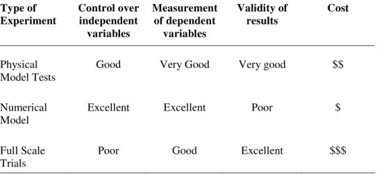
In practice, the most effective means of developing a model for use in DP control and related applications is to use a combination of all of the approaches that have been described above. As summarized in Table 1, each of the approaches has strengths and weaknesses. In the life-cycle of developing a useful model, each experimental technique can often be used in parallel. In general, the lowest cost experiment
(numerical modeling) should be used the most, while the most expensive (full scale trials) should be used less frequently. It should be noted that the results of numerical models are the least trustworthy, so these should be only relied upon once they have been validated by a more trustworthy source, either model or full scale experiments (i.e. validation).
At IOT, the approach has been to conduct model scale experiments and, in parallel, construct numerical models. We are currently comparing the numerical modeling results to specific model test scenarios to validate the modeling tools we have developed. In the following sections, each of these approaches will be described in some more detail.
Table 1: Comparison of model types for DP system performance evaluation. Type of Experiment Control over independent variables Measurement of dependent variables Validity of results Cost Physical Model Tests
Good Very Good Very good $$
Numerical Model
Excellent Excellent Poor $
Full Scale Trials
Physical Modeling
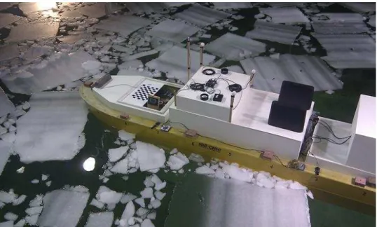
IOT has been carrying out physical model testing in order to quantify ice loads on a dynamically-positioned vessel in simulated managed ice conditions. For modeling of stationkeeping applications, the pack ice moved and the vessel stands still. Since this is not easy to recreate without a flume tank and an endless supply of ice, the vessel is moved through the stationary ice field. The result is essentially the same, if the speed of the vessel is set to be the desired drift speed of the ice, then the pack ice
encountering the hull has the correct relative drift speed.
Figure 2: Model DP drillship in IOT's ice tank (August 2011).
The model that is pictured in Figure 2 was designed to approximate a large drillship or FPSO at a scale in the range of 1:30 to 1:40. At a scale of 1:40, the model represents a full scale vessel that is 200 m LOA, has 40 m beam and that displaces around 100,000 tonnes. For propulsion, the model is equipped with 6 azimuthing thrusters that at full scale would generate around 8 MN of propulsion total. For model testing, the response time of thrusters and maximum thrusts must be carefully modeled to ensure similitude to the full-scale vessel.
Model Dynamic Positioning System
In order to have complete control over the independent variables of the test, IOT uses an in-house DP system that is designed with non-proprietary control technology. This is an important factor in the
validation of the test results, since proprietary, “black-box” DP control algorithms may not be comparable from manufacturer to manufacturer and may potentially influence the test results in unexpected ways. IOT’s model DP system allows for testing of models without tethering (free-running tests). All
communications to and from the model are done via wireless systems and the model has a self-contained power source that has sufficient storage to power the model for more than a day of testing. In our experience, umbilical systems for models can influence the model motion. Although the force imparted on the model by an umbilical is small, it may have a significant effect in ice testing due to the sensitivity of these tests to initial conditions.
All internal DP calculations, including state estimates from Kalman filters, error signals, control demands, and thruster settings are available to be recorded. In Fig. 3 the results of a DP vessel operating in pack ice drifting at 1 knot full scale speed are presented. These plots show the excursion of the vessel from the desired station (setpoint of 30,-5 meters, and heading angle 0 degrees). At full-scale, this record represents around an hour of operation.
Figure 3: A typical data product from a model test that shows how well the vessel held station in drifting ice (results are scaled to full scale).
Ice Conditions
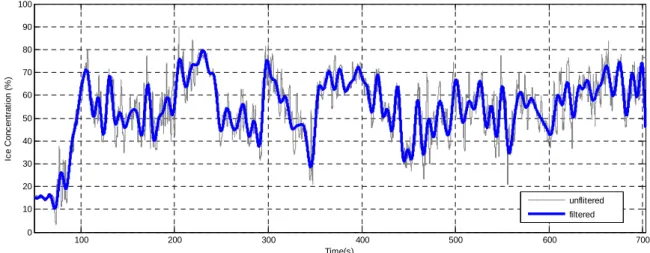
Measuring and recording the ice field that the vessel encounters as it moves down the tank is of the utmost importance, since we are attempting to find a relationship between characteristics of the ice field and the forces and moment that the DP system uses to maintain station. IOT has developed a machine-vision system that images, analyzes and records the ice conditions surrounding the vessel in real time. Some parameters that can be generated by this system are concentration, and statistical quantities regarding the ice pieces within defined areas surrounding the vessel. This information is essential to the analysis of the model test results and to defining, reproducing and correlating results with the numerical models.
Figure 4: Machine vision system with thresholded image of ice on the left and edge detection on the right. 100 200 300 400 500 600 700 0 10 20 30 40 50 60 70 80 90 100 Time(s) Ic e C o n c e n tr a ti o n ( % ) unflitered filtered
Figure 5: Concentration as a function of time computed by the ice machine vision system.
Numerical Simulation
The purpose of the numerical simulation is to predict ice loads cost effectively associated with model testing. As the first step, numerical model needs to be validated with model test data. Once the model is validated, a wide range of ice conditions and vessel’s operating conditions can be simulated to estimate ice loads with reasonable accuracy. At this stage, we will use model test data to evaluate the numerical model: agreement between the two modeling techniques increases confidence in the correctness of both techniques because the results were arrived at it in completely different ways.
Numerical Setup
Fig. 6 shows the numerical domain for simulation using commercial Finite Element Code, LS-DYNA. It consists of water, air, ship and ice pieces. Ice pieces were roughly imitated from the still cut of the video
but it will be more accurately and automatically generated using the ice machine vision system described in the previous section. This feature is currently undergoing testing and was not complete at the time of writing.
Figure 6: Numerical domain of vessel, ice and water.
For this simulation, ship and ice were modeled as a rigid body with no dynamic positioning system applied. Essentially, the vessel in the simulation is towed by a virtual tow carriage (only surge motion is allowed), forcing the vessel to move smoothly.
This simulation is at a preliminary stage and it shows the future plan for numerical analysis, which is to improve ice load predictions for both the numerical and the physical models. Figs 7-9 show the rough visual comparison between numerical simulation and model testing. In future steps, the numerical model should have a model of the DP system as part of its dynamics and should be free to move in all three axes: i.e. sway and yaw, in addition to surge.
Scale of Numerical Models
Numerical models were created in LS-DYNA for both a model scale vessel and a full-scale vessel in order to understand the differences that might occur due to scale effects. The primary expected difference between full scale and model scale behaviour is with the ice movement, as at model scale, the drift movement is dominated by fluid forces which do not scale well at model scale. This is a well-known issue with physical modeling: fluid drag forces are more correctly modeled using Reynolds scaling, while the model tests are designed around Froude scaling as they hold well for hydrodynamics, propulsion and other related phenomena.
In Figs. 7 – 9, we see the results of a physical model test on the right hand side and the results of the numerical model on the left. This shows reasonably good agreement between the two out to 20 seconds, with ice piece motion working reasonably well (moving, tilting and sliding).
Figure 7: Numerical simulation (left) and model testing (right) before starting
Figure 8: Numerical simulation (left) and model testing (right) after 10 seconds
Conclusions
In the near future, DP-equipped vessels operating in ice-covered waters will become more commonplace. DP stationkeeping operations in managed ice will owe their success in a large part to the ability of the control system to anticipate ice loading/unloading on the vessel’s hull and to deal with these events appropriately.
In addition to helping DP system performance, the development of numerical models of how these global ice loads impact a vessel will enable designers to assess performance and determine safe operating limits. These models can also be used to construct realistic simulation environments for operator training and for development of operational scenarios.
The best approach to developing a validated numerical model is to rely on both full-scale data and model scale data. Unfortunately, full-scale data for vessel stationkeeping in ice is rare and generally proprietary. Model scale testing provides a relatively low-cost way of testing the limitations of stationkeeping systems in ice as well as providing validation to the numerical modeling.
Bibliography
1. Ljung, L., System Identification: Theory for the User, Prentice Hall, 1987. 2. Ogata, K., Modern Control Engineering, Prentice Hall, 4th Ed., 2002. 3. Khalil, H. K., Nonlinear Systems, Prentice Hall, 3rd Ed., 2002.
4. Fossen, T.I., Guidance and Control of Ocean Vehicles, John Wiley & Sons, 1994. 5. Fossen, T.I., Marine Control Systems, Marine Cybernetics, 2002.
6. Palm, W.J., Modeling, Analysis and Control of Dynamics Systems, Second Ed., 1999. 7. Grewal, M and Andrews, A., Kalman Filtering Theory and Practice, Prentice Hall, 1993.