Publisher’s version / Version de l'éditeur:
Vous avez des questions? Nous pouvons vous aider. Pour communiquer directement avec un auteur, consultez la première page de la revue dans laquelle son article a été publié afin de trouver ses coordonnées. Si vous n’arrivez pas à les repérer, communiquez avec nous à [email protected].
Questions? Contact the NRC Publications Archive team at
[email protected]. If you wish to email the authors directly, please see the first page of the publication for their contact information.
https://publications-cnrc.canada.ca/fra/droits
L’accès à ce site Web et l’utilisation de son contenu sont assujettis aux conditions présentées dans le site LISEZ CES CONDITIONS ATTENTIVEMENT AVANT D’UTILISER CE SITE WEB.
The 23nd International Congress on Applications of Lasers & Electro-Optics
(ICALEO) 2004 [Proceedings], 2004-10-08
READ THESE TERMS AND CONDITIONS CAREFULLY BEFORE USING THIS WEBSITE.
https://nrc-publications.canada.ca/eng/copyright
NRC Publications Archive Record / Notice des Archives des publications du CNRC : https://nrc-publications.canada.ca/eng/view/object/?id=880bb8db-ed00-4c52-a00d-c238cfaaa28b https://publications-cnrc.canada.ca/fra/voir/objet/?id=880bb8db-ed00-4c52-a00d-c238cfaaa28b
NRC Publications Archive
Archives des publications du CNRC
This publication could be one of several versions: author’s original, accepted manuscript or the publisher’s version. / La version de cette publication peut être l’une des suivantes : la version prépublication de l’auteur, la version acceptée du manuscrit ou la version de l’éditeur.
Access and use of this website and the material on it are subject to the Terms and Conditions set forth at
Optimization of Aluminium Laser Welding Using Taguchi and EM
Methods
IMI2004-105433-g CNRC4695&
Optimization of aluminium laser welding using Taguchi and EM methods
L. DUBOURGa,l, B. DES ROCHEsa, A. COUTUREb, D. BOUCHARDa ,H. R. SHAKERIa
a Aluminium Technology Centre, National Research Council Canada, 501 Boul. de I'Universite, Saguenay (Quebec) Canada, G7H 8C3
b REMAC Inc., 2953 boul. du Royaume, Saguenay (Quebec) Canada, G7X 7V3 I Corresponding author: Tel. +1 418 545-5098; Fax + 1418545-5345
E-mail: [email protected] (L. Dubourg)
ABSTRACT
Effect of laser welding parameters such as power, out-of-focus length, speed, diameter of feeding wire and feeding speed on weld properties are studied. The process parameters and their respective and interactive effects on the final responses have been investigated simultaneously by minimizing the number of experimental runs. The results, indicating the interlateral relationship between laser process parameters and responses, have been used to optimize the laser parameters, to predict the responses and to increase the process robustness. Two millimetre thick plates of AA6061 were welded in fillet configuration using a cw/Nd:Y AG laser and AA5356 wire as the filler metal. Two different experiment-designing methods were used and compared to find the most efficient way to optimize laser welding. The Taguchi method that allows a multicriteria optimization, using orthogonal arrays, was used to reduce the number of trials necessary to cover the whole functional process parameters window. The same kind of optimization was then carried out with E.M. method in a more interactive way allowing a dynamic construction of the feasible domain throughout the data collection. The weld properties of interest were weld fillet size, penetration depth, concavity size and HAZ dimensions.
1. INTRODUCTION
Many studies conducted on laser welding have shown that a number of process parameters could affect properties of welds. Effects of nature as well as volumetric flow rate of the shielding gas (1, 2), laser power (1, 2), welding speed (1-4), and out-of-focus length (4, 5) on one or more of the properties such as porosity, keyhole stability, weld geometry, hot cracking, depth of penetration, loss of alloying elements due to evaporation and the size of HAZ have been investigated. Most studies are based on butt-joint and bead-on-plate welding without using any filler. In instances where a large number of parameters need to be considered, the use of design of experiment (DOE) is highly recommended. In most welding applications, full factorial designs are traditionally used. In such designs that vary one factor at a time, the number of runs increases dramatically with the number of parameters and levels. With multi-variant methods, many factors can be simultaneously varied that minimizes the number of runs. The Taguchi method is based on an orthogonal array system and leads to a design where the effect of every parameters can be evaluated in far fewer runs (6, 7). This method has several advantages, but also some limitations. New multi-variant methods have been developed based on alternative principles, which solve some of the problems in Taguchi method. Authors have already compared Taguchi method with D-optimal (8). In the present study, the optimization of the number of runs was done using both Taguchi and E.M. (9, 10). The latter technique is based on building an Euclidian domain and modifying it in an interactive way, varying all the parameters at the same time. This method has already been used in arc welding (11). The objective of this investigation was to identify the process parameters that affected most the welds and their proper settings. This was done using both Taguchi and E.M. methods. A statistical model and multicriteria optimisation was performed to get the overall optimum of the process parameters. Finally, two methods as well as the obtained results were compared.
2.EXPERIMENTAL PROCEDURE
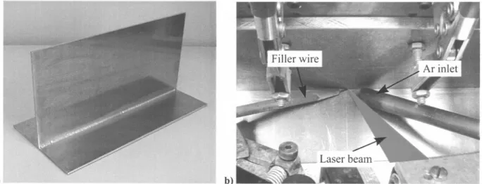
ANd: YAG laser of 1.064-f.tm wavelength and a 600 f.tmdiameter optical fibre operating in continuous wave regime was used. A 200-rom focal length lens with 0.6 mm spot diameter at the focal point was used. Plates of 2-mm thick AA6061 were welded in fillet configuration (Fig. l.a). Optical fibre of the laser, shielding gas and wire filler delivery systems were controlled using a Fanuc multi-axis robotic arm. The angle between the laser beam and the horizontal plate maintained at 45°. The laser was pointed towards the edge of the joint formed by the two plates with an angle of 15° with respect to a plane perpendicular to that edge (Fig. l.b). Normal incidence was avoided to minimize beam reflections, which could damage the optical fibre or the laser chamber. Argon was used as the shielding gas and was injected through a copper nozzle at a 45° angle with respect to axis of the laser using a volumetric flow rate of 25 l.min". AA5356 filler wires of 1.2 and 1.6 rom diameter were fed at a 60° angle relative to laser axis. The plate surface was degreased with acetone to eliminate hydrogen compounds, which could lead to the occurrence of porosity (5).
--a)
I
.
b)Figure 1: a) sample after welding, b) experimental set-up.
iIIi
'*
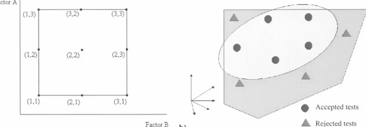
The influence oflaser welding parameters such as power, out-of-focus length, welding speed, wire diameter and wire feeding speed on weld properties were studied. Two different DOE methods (Taguchi and EM) were used and compared in order to find the better way to optimize laser welding parameters. The Taguchi method relies on a system based on a normalized orthogonal matrix. Each set of matrix assures that the space will be investigated in a way that the effect of every variable can be detected without mixing them up (although secondary and higher order interactions may be confounded). This could be done by varying many parameters at the same time along the orthogonal border of the orthogonal domain. The number of factors and possible levels for each factor determine the size of the orthogonal domain. Fig. 2.a shows a L9 matrix for 2 factors with 3 levels. In this case, it is equivalent to a traditional factorial design with 32trials. With a L9 matrix, like the case in this study, it is possible to study 4 factors at three levels each in only nine trials. A one at a time factor design would otherwise take 34 trials. In this study, 2 steps ofL32 design reduced the 1024 (45)trials requested by a factorial design down to 64 trials. Alternatively, E.M. technique is based on building a Euclidian domain and modifying it in an interactive way, varying all the parameters at the same time. The feasible domain in the process that is defined by the multidimensional volume in a continuous factor space best discriminates between accepted tests inside this volume and rejected tests that are outside. Fig. 2.b illustrates the feasible domain. This domain is built test after the test and the selection of each subsequent test is based on maximizing the gain in new information. If the test is accepted, based on predefined criteria, the domain will be redefined to take into account this new direction of investigation. But if the test were rejected, the boundaries of the domain in this direction and causes of rejection would be identified. This method allows a more interactive approach through dynamic construction of the feasible domain throughout the data collection. In the present study, a combination of Taguchi and EM methods were used. As the first step, a L32 Taguchi matrix was used to promptly define the feasibility domain and to explore efficiently the multidimensional volume. Subsequently, the EM method
was used to refine the domain and to find the key indictors that could explain the variations of the responses and to build a stable equation with good analytical capability.
Factor A
A
/"""---8 8'\,/
//
Y
)
A
/
, . ."8
8
{(
I
\8
I \/
~
"-~ . 1.-
.-
J
./'~
/-(
/~~
~'... ,---~/ 8 Acceptedtestsa) FactorB b)
~
Rejected testsFigure 2: a) Example of Taguchi method: L9 design for 2 factors at 3 level each, b) Example of E.M. method: feasible domain of the process.
(1,3) (3,2) (3,3)
(1,2) (2,2)
.
(2,3)(1,1) (2,1) (3,1)
In order to characterize the welds, 4 responses were analysed. The weld geometry was evaluated using an optical microscope. Four dimensions were measured for each sample as shown in Fig. 3. The height (H) and width (L) of the weld were measured as well as the average size defined as (H+L)/2. The distance from the junction of the two plates to the most distant weld point in the matrix was used to quantify penetration (P). Finally, a triangle of height Hand width L was drawn. The hypotenuse of this triangle represents a flat weld of same dimension as the actual weld. The distance (C) in this case is the largest gap between this hypotenuse and the weld surface. It was given a negative value for a concave shape, as seen on Fig. 3, and a positive value for a convex weld. The last parameter analyzed was the size of the heat-affected zone (HAZ). An advantage oflaser welding is that it produces a narrow HAZ compared to traditional techniques like arc welding due to its lower heat input (2). Several authors (3) reported HAZ in
AA6061alloy as well as alloys of other heat-treatableseries during laser welding.Microhardnessmeasurements
were used to determine the size of the HAZ. For microhardness a 50g load, applied for 5 seconds, was performed to obtain hardness profiles throughout the specimen.
Figure 3: Dimensions measured for weld's characterization
3. RESULTS
3.1 Design of experiments
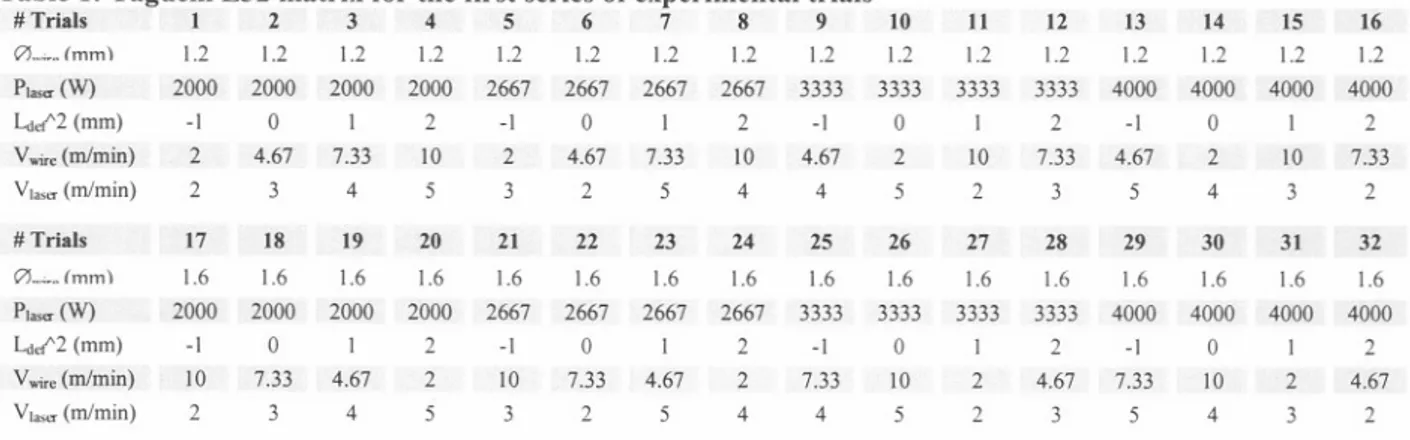
With the Taguchi method, a L32 matrix was used in the first step, combining 5 input parameters for a total of 32 trials (Table I). We used one 2-level input parameter (wire filler with diameters of 1.2 and 1.6mm) and four 4-level
parameters: power (ranging from 2000 to4000W), out-of-focuslength(rangingfrom -1 to 2 mm, negativelength
meaning a focal point within the matter), filler wire speed (from 2 to 10 mlmin) and welding speed (between 2 and 5 mlmin). After analysing the primary results, the orthogonal space generated using the previous design was assumed to be too large since 13 of the 32 scheduled trials had failed. It was then decided to reduce the range of process parameters. Most of the failures happened with the 1.6mm wire and were to the lower levels of power. From this first observation, it was concluded that the minimum power limit should be higher. Some failure cases also corresponded to higher wire feeding speed and welding speed. In both cases, the appropriate speed seemed to be different for each wire diameter. An L9 design was then selected for each wire diameter (1.2 and 1.6 mm). For 1.2 mm, laser power (2300,2800,3300 W), out-of-focus length (-1, 0, 1 mm), wire filler speed (3, 5, 7 mmImin) and welding speed (2,3, 4 mmImin) were the 4 remaining input parameters and 3 levels were selected for each one of them. For 1.6mm, the input parameters were set as follows: laser power: 2800, 3200 and 3600 W, out-of-focus length: -0.5,0.75 and 2 mm, wire feeding speed: 2, 4 and 6 mmlmin, welding speed: 2, 3 and 4 mmImin.
For the EM method, 2 steps were considered. In the first step, the same Taguchi L32 matrix as shown in Table 1 was used. This step promptly defined the feasibility domain and explored efficiently the multidimensional volume. In the second step, the interactive way of the E.M. technique was used, i.e. varying all the parameters at the same time. The domain was built test after the test and each subsequent test was selected in such way to maximize the gain in new information. If the test was accepted, the domain was redefmed to take into account this new direction of investigation. But if the test were rejected, the domain boundaries in this direction and the causes of rejection would have been identified. This method takes a more interactive approach leading to the dynamic construction of the feasible domain throughout the data collection. This reduces the number of tests from 50 with the Taguchi method alone to 42 with the combination of the 2 DOE methods. The number of tests was reduced by around 16%. Moreover, as shown in Table 2, the prediction equations obtained from EM were stable and were similar to the ones obtained from Taguchi.
3.2 Process modelling
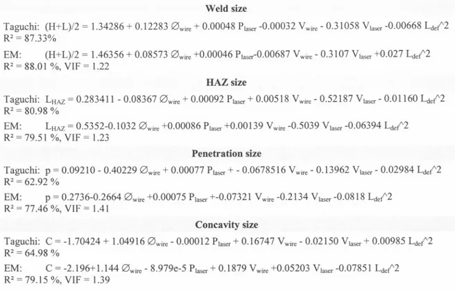
The regression equations of the table 2 show the modeling of the different responses as function of the input parameters for both methods. For all equations, we noted stable R2 regression coefficients higher than 70%, leading to a good analytical power. Moreover, in the EM equations, it could be seen that calculated variation inflation factors (VIF) is close to I. These factors measure how much the variance is increased relative to the case when all of the factors are uncorrelated. These VIF values assess the stability of the regression coefficients. VIF = 1 for independent predictors. VIF values above 5 are not acceptable. A VIF value exceeding 5 indicates that the regression coefficients are poorly estimated because of multicolinearity and regression coefficients are unstable (J0). (equivalent avec Taguchi ???). Moreover, regression equations obtained using the EM method were similar to the ones obtained using Taguchi, in spite ofa significant reduction of the test number.
Table 1: Taguchi L32 matrix for the first series of experimental trials
# Trials 1 2 3 4 5 6 7 8 9 10 11 12 13 14 15 16 0...lmm\ 1.2 1.2 1.2 1.2 1.2 1.2 1.2 1.2 1.2 1.2 1.2 1.2 1.2 1.2 1.2 1.2 PI...,.(W) 2000 2000 2000 2000 2667 2667 2667 2667 3333 3333 3333 3333 4000 4000 4000 4000 L.Jef'2 (mm) -I 0 1 2 -I 0 I 2 -J 0 1 2 -I 0 I 2 Vwire(mlmin) 2 4.67 7.33 10 2 4.67 7.33 10 4.67 2 10 7.33 4.67 2 10 7.33 VI"" (mlmin) 2 3 4 5 3 2 5 4 4 5 2 3 5 4 3 2 # Trials 17 18 19 20 21 22 23 24 25 26 27 28 29 30 31 32 0..,...lmm\ 1.6 1.6 1.6 1.6 1.6 1.6 1.6 1.6 1.6 1.6 1.6 1.6 1.6 1.6 1.6 1.6 P1...,.(W) 2000 2000 2000 2000 2667 2667 2667 2667 3333 3333 3333 3333 4000 4000 4000 4000 L.Jef'2 (mm) -I 0 J 2 -I 0 1 2 -I 0 1 2 -I 0 1 2 Vwire(mlmin) 10 7.33 4.67 2 10 7.33 4.67 2 7.33 10 2 4.67 7.33 10 2 4.67 VI...,. (mlmin) 2 3 4 5 3 2 5 4 4 5 2 3 5 4 3 2
Table 2: regression equations of responses as a function of the input parameters for the Taguchi and EM methods.
Weld size
Taguchi: (H+L)/2 = 1.34286 + 0.122830wire + 0.00048 Pla50r-0.00032 Vwire- 0.31058 Vla50r-0.00668 Lde{'2
R2 = 87.33%
EM: (H+L)/2 = 1.46356 + 0.08573 0wire +0.00046 Plaser-0.00687 Vwire- 0.3107 Vlaser+0.027 Lde{'2
R2= 88.01 %, VIF = 1.22
HAZ size
Taguchi: LHAZ
=
0.283411 - 0.083670wire + 0.00092 Plaser+ 0.00518 Vwire- 0.52187 Vlaser- 0.01160 Lde{'2R2= 80.98 %
EM: LHAZ= 0.5352-0.1032 0wire +0.00086 Plaser+0.00139 Vwire-0.5039 Vlaser-0.06394 Lde{'2
R2= 79.51 %, VIF = 1.23
Penetration size
Taguchi: p = 0.09210 - 0.40229 0wire + 0.00077 Plaser+ - 0.0678516 Vwire- 0.13962 Vla50r- 0.02984 Lde{'2
R2= 62.92 %
EM: p = 0.2736-0.2664 0wire +0.00075 Plaser+-0.07321 Vwire-0.2134 Vlaser-0.0818 Lde{'2
R2= 77.46 %, VIF = 1.41
Concavity size
Taguchi: C = -1.70424 + 1.049160wire - 0.00012 Plaser+ 0.16747 Vwire- 0.02150 Vlaser+ 0.00985 Lde{'2
R2 = 64.98 %
EM: C = -2.196+ 1.144 0wire - 8.97ge-5 Plaser+ 0.1879 Vwire+0.05203 Vlaser-0.07851 Lde{'2
R2= 79.15 %, VIF = 1.39
Fig. 4 and 5 show the Pareto charts for each response as a function of the input parameters. The Pareto chart is an illustration of the estimated effects of the predictors. The length of each bar on the chart is proportional to the positive or negative standardized effect. According to Fig. 4.a, weld average size is correctly predicted by the welding speed (Vlaser)and the laser power (P). This leads to the following conclusions. (i) The weld size is only a function of the laser power and the welding speed, i.e. the linear energy input. (ii) Wire feeding speed (Vwire)and wire diameter (0wire) do not influence the weld size. This came as a surprise since the couple (Vwire- 0wire) represents the quantity of filler material. These observations, led to the conclusion that for each couple (Vlaser
-
P)there is a corresponding single couple (Vwire
-
0wire), which can lead to a correct weld. (iii) The focus point position does not influence the weld size.The HAZ size is predicted by the same input parameters and with the same standardized effects as seen on Fig. 4.b. This leads to the following conclusions. (i) The HAZ size is only a function of the laser power and the welding speed, i.e. the linear energy input. (ii) HAZ size is proportional to the weld size. A small weld leads to a small HAZ zone.
Welding speed 18J+
.-
Welding speed.+
8-Laser power Laser power
Out-of-focus'2I
I
Wire diameterII
Wire speed I~ Out-of-focus'210
Wire diameter!I
Wire speedII
0 4 8 12 16 a 3 6 9 12 Standardizedeffect 15 Standardized effect a) b)Figure 4: Pareto chart for a) weld average size (H+L)/2, b) HAZ size (LHAZ).Highest-order effect is 2.
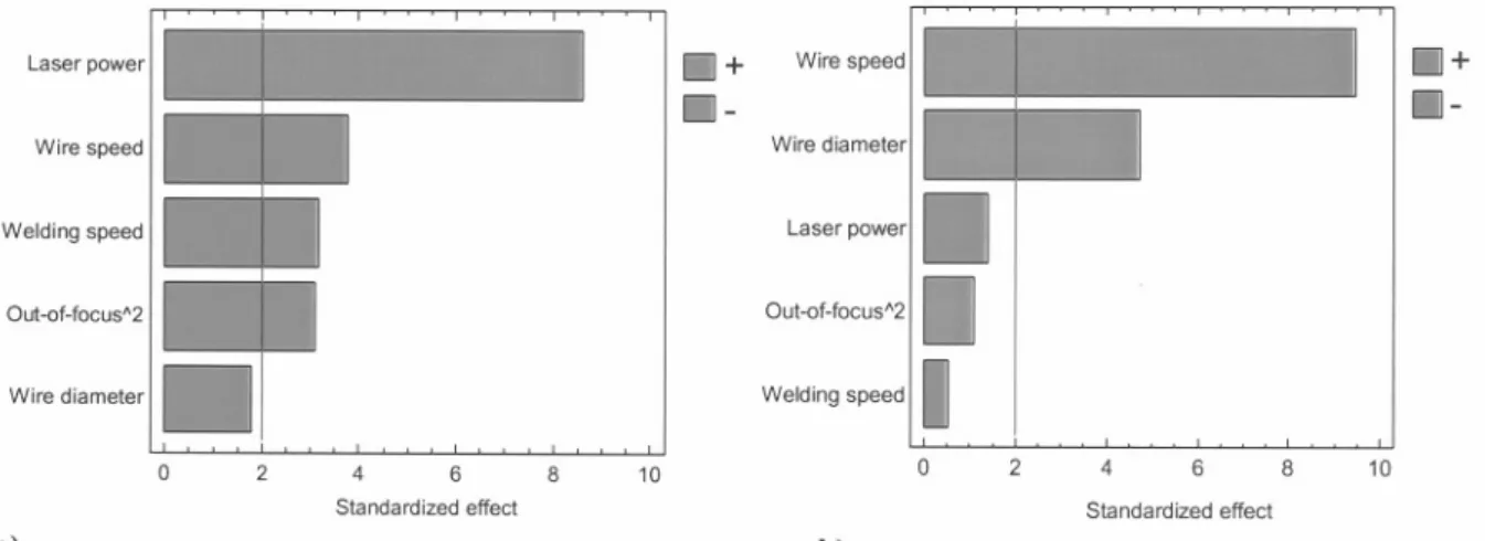
The laser power, the wire speed, the welding speed and the square of the out-of-focus length, i.e. the area of the beam spot, can predict depth of penetration (see Fig. 5.a), but the most meaningful input parameter is still the laser power. In the case of the concavity size, wire speed and wire diameter, i.e. the feed material quantity, are most influential (seeFig. 5.b).
Laser power
.+
.-
Wire speed.+
8-Wire diameter Wire diameterI
.
Laser powerl.
Out-of-focus'21.
Welding speedII
Welding speed Out-of-focus'2 0 2 4 6 8 10 0 2 4 6 8 10Standardized effect Standardized effect
a) b)
Figure 5: Pareto chart for a) penetration depth (p), b) concavity size (C). Highest-order effect is 2.
3.3 Process modelling
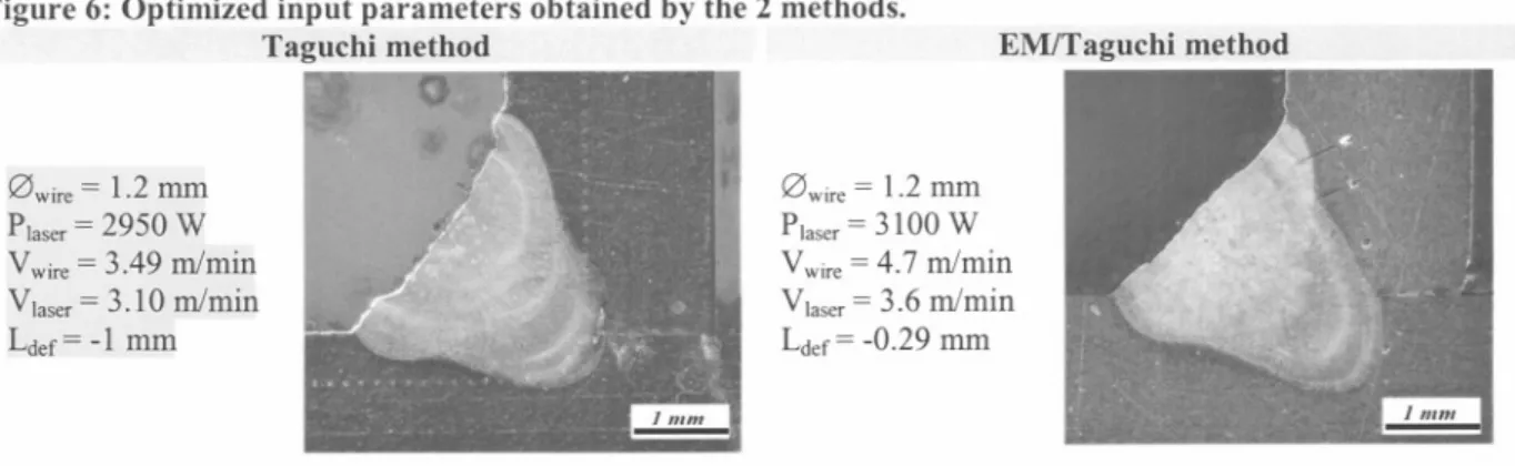
The previous process modeling (Table 2) was used to find the process parameters most optimized and robust for the both method. The optimization criteria were defined as follows: weld average size was targeted of 1.9 mm, HAZ was minimized to 0 mm, concavity size was targeted of 0 mm and penetration depth was minimized to 0 mm. Fig. 3 shows the optimized input parameters obtained by the Taguchi alone and the combination of Taguchi and EM The cross sections of the welds obtained with these optimized parameters are also shown. These results are very close; nevertheless, we noted that the optimized parameters obtained with Taguchi + EM were slightly higher than those obtained with Taguchi alone. This leads to a higher penetration depth.
Figure 6: Optimized input parameters obtained by the 2 methods.
Taguchi method EM/Taguchi method
0wire = 1.2 mm Plaser= 2950 W Vwire= 3.49 mlmin Vlaser= 3.10 mlmin Ldef= -1 mm 0wire = 1.2 mm Plaser= 3100 W Vwire= 4.7 mlmin Vlaser= 3.6 mlmin Ldef= -0.29 mm 4. DISCUSSION
The Taguchi method covers more than just the creation of a plan of experiments. In the present case, only the orthogonal matrix system generated by this method was used. This matrix allows examination of the space bounded by the defined limit levels for each input parameter. Moreover, this ensures that every single point so defined will lead to the identification of the effect of each variable on the response. Taguchi method can lead to a significant reduction in the number of experiments in many cases. The extent of this reduction depends on the number of input parameters and levels. These two components are used to select one matrix from the set of available matrices. In some cases, the number of experiments may be superabundant while in other cases, each experiment becomes critical and each point becomes essential in order to isolate the effect of each parameter. With a matrix built with the Taguchi method, extreme points in the space defined from the imposed parameters limits are always included in the trial runs. When more than two levels are chosen for the process parameters, intermediate points may also be investigated. However, with the Taguchi method, the experimental trials are preferentially located at the space boundaries to use the maximum of the matrix capabilities. In the particular case of welding experiments, certain combinations of parameters led to failed tests. The statistical analysis becomes more difficult because the information given by the failed tests is not easily described. Moreover, orthogonal matrices bound a regular and totally symmetrical space. If a region of this space needs special interest, it is always possible to add more points to this region. However, in case of processes like welding, the number of input parameters could be very large and it became difficult to identify an interesting sub-space in a four- or five-dimension space. Table 3 summarizes the advantages and drawbacks of Taguchi method that we found during this laser welding study.
Table 3: advantages and drawbacks of Taguchi method. Advantages
- Build a plan make sure that the effect of each parameter is taken into account
-
Leads to a fixed design plan, which is easy to follow- Leads to a systematic work plan (DOE, experimentation, measurements and analysis) - Possibility of mixing with other designs and adding points
- Allows multicriteria optimization
-
Explores the boundaries of a domain which can be useful to initialise an experimental campaign Drawbacks- Produces an orthogonal domain that is symmetric but this does not necessarily correspond the real domain
-
Preferable to have an apriori knowledge of the process in order to minimize failed tests-
Ifa test fails and cannot be analysed, there's a risk of missing the effect of some input parameters. - The design cannot be changed during the experimentEM is an interactive method, building of an elliptic domain (Euclidian geometry). This allows visualization of five-dimension spaces and identification of portions of this space yet to be explored. Points could be added anywhere, which allows examination of this space in a totally asymmetrical way with an emphasis on certain areas. Even when an experiment fails, it still comprises useful information since it could be further visualized that allows identification of non-exploitable zones not in the space. As far as domain building is concerned, EM presents an interesting aspect but with some limitations. It is effectively advantageous to be able to experimentally circumscribe the feasibility domain and to trace a limit. However, the elliptical domain does not always correspond to a real domain shape and during domain building, zones of interest may be excluded from the domain or zones with little interest might end up
being included in it. Even so, the ellipsoid remains a valuable reference and if it cannot represent the domain accurately, it can, according to the building criteria, define a zone into which one can be assured obtaining satisfying results. Moreover, with EM, there is no plan of experiments as such. Consequently, it might be difficult to explore a four-plus-dimension space, even with the help of the visualization system. Furthermore, there is no means to be sure that the selected runs would permit isolating the influence of each one of the parameters. For the EM method, Table 4 summarizes the advantages and drawbacks that we observed during these tests.
Table 4: advantages and drawbacks of EM method.
Advantages
-
Interactive domain building can lead to a lower number of experiments-
Possibility of mixing with other DOE-
Allows multicriteria optimization-
Interactive domain building is more likely to study irregular feasible domain-
Possibility to fit in an orthogonal DOE in it.Drawbacks - Does not lead to a fixed experimental plan
-
Results of previous experiments must be known to build feasible domain and to pursue experimentation. This can take time in the case of metallurgic preparation.- Euclidian geometry does not fit any domain. It depends of the specifications.
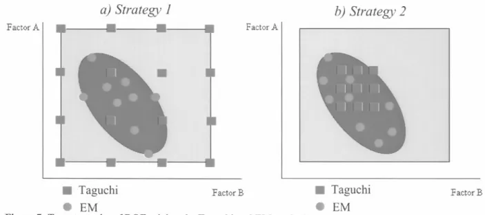
Concerning data analysis, both methods are comparable. Model building is based on regression analysis and similar statistical methods lead to the identification of the significant variables. Finally, mixing both methods was interesting. Two different strategies of mix could be adopted depending on the number of experiments that could be done (Fig. 7). The first one used in this study, consists in selecting wide limits on input parameters with numerous levels for each and using an orthogonal matrix (see Fig. 7.a). In this case, one could be assured to cover a large area of the space. The results could then be analyzed with the EM method to build a domain and to decide if more experiments are still needed. EM allows judicious selection of the new points in order to maximize the information gain (Fig. 7.a). In the present case, it translated into a reduction by 16% of the number of experiments while still determining the behaviour models for the process. This first strategy is mostly efficient when it is possible to complete a large number of experiments (42 in the present case) and also when the process behaviour is unknown. On the contrary, if the limits of the process are fairly known, the second strategy consists in limiting the variation of the input parameters and their levels and selecting an orthogonal matrix with a smaller number of experiments that for each run offers a good possibility of success (see Fig. 7.b). Afterwards, to explore new possibilities with the EM method requires enlarging the domain through running additional experiments (Fig. 7.b).
Factor A
a) Strategy 1
.
b) Strategy 2
FactorA
.
. Taguchi
Factor
B
. Taguchi
. EM
. EM
Figure 7: Two strategies of DOE mixing the Taguchi and EM methods.
5. CONCLUSION
The present work studied the influence of various laser welding parameters such as power, out-of-focus length, welding speed, wire diameter, and wire feeding speed on weld properties. Plates of 2-mm thick AA6061 were welded using a cw/Nd:YAG laser in fillet configuration with AA5356 wire as the filler metal. The weld properties of interest were weld fillet size, depth of penetration, concavity size and HAZ dimensions. Two different experiment design methods were used (Taguchi and TaguchilEM) and compared in order to find the most efficient way to optimize laser welding. The classic Taguchi method that allows a multicriteria optimization using orthogonal arrays was used to reduce the number of trials necessary to cover the whole functional process parameters window. Combination of Taguchi and EM methods promptly define the feasibility domain, explore efficiently the multidimensional volume and build dynamically of the feasible domain throughout the data collection. Both strategies provided equivalent prediction models for the optimised process parameters but the second required approximately 16% less experimental tests. The process parameters and their respective and interactive effects on the final responses have been investigated. The results, expressing the interrelationship between laser process parameters and responses, have been used to optimize the laser parameters, to predict the responses and to increase the process robustness.
REFERENCES
1. G. Casalino, L. A. C. De Filippis, A. D. Ludovico, paper presented at the 20th International Congress ICALEO 2001, Jacksonville, FL 2001.
C. Mayer, F. Fouquet, M. Robin, Materials Science Forum, 217 (1996). M. Kutsuna, Q. Yan, WeldingInternational 13, 597 (1999).
M. Pastor, H. Zhao, T. Debroy, WeldingInternational 15, 275 (2001).
A. Haboudou, P. Peyre, A. B. Vannes, G. Peix, Materials Science and Engineering A 363, 40 (2003). Y. S. Tamg, W. H. Yang, International Journal of Advanced Manufacturing Technology 14, 549 (1998). K. A. Kloss, paper presented at the Advances in Welding Technology, 11th Annual North American Welding Research Conference, Columbus OH, 7-9 Nov 1995 1996.
S. Subramaniam, D. R. White, J. E. Jones, D. W. Lyons, WeldingJournal 78, 166 (1999).
M. Galopin, T. M. Dao, 1. P. Boillot, paper presented at the 4th International Conference of Computer Technology in Welding, Cambridge, UK, 3-4 June 1992.
M. Galopin, S. Hansquine, T. M. Dao, C. Q. Zheng, paper presented at the High-Productivity Joining Processes, ICAWT '97 International Conference Advances in Welding Technology, Columbus, 17-19 Sept. 1997.
M. Galopin, J. P. Boillot, G. Begin, paper presented at the Recent Trends in Welding Science and Technology, Gatlinburg, TN, 14-18 May 1989.
2. 3. 4. 5. 6. 7. 8. 9. 10. 11.