Publisher’s version / Version de l'éditeur:
Urban Water, 3, September 3, pp. 131-150, 2001-09-01
READ THESE TERMS AND CONDITIONS CAREFULLY BEFORE USING THIS WEBSITE.
https://nrc-publications.canada.ca/eng/copyright
Vous avez des questions? Nous pouvons vous aider. Pour communiquer directement avec un auteur, consultez la première page de la revue dans laquelle son article a été publié afin de trouver ses coordonnées. Si vous n’arrivez pas à les repérer, communiquez avec nous à PublicationsArchive-ArchivesPublications@nrc-cnrc.gc.ca.
Questions? Contact the NRC Publications Archive team at
PublicationsArchive-ArchivesPublications@nrc-cnrc.gc.ca. If you wish to email the authors directly, please see the first page of the publication for their contact information.
NRC Publications Archive
Archives des publications du CNRC
This publication could be one of several versions: author’s original, accepted manuscript or the publisher’s version. / La version de cette publication peut être l’une des suivantes : la version prépublication de l’auteur, la version acceptée du manuscrit ou la version de l’éditeur.
For the publisher’s version, please access the DOI link below./ Pour consulter la version de l’éditeur, utilisez le lien DOI ci-dessous.
https://doi.org/10.1016/S1462-0758(01)00033-4
Access and use of this website and the material on it are subject to the Terms and Conditions set forth at
Comprehensive review of structural deterioration of water mains: statistical models
Kleiner, Y.; Rajani, B. B.
https://publications-cnrc.canada.ca/fra/droits
L’accès à ce site Web et l’utilisation de son contenu sont assujettis aux conditions présentées dans le site LISEZ CES CONDITIONS ATTENTIVEMENT AVANT D’UTILISER CE SITE WEB.
NRC Publications Record / Notice d'Archives des publications de CNRC:
https://nrc-publications.canada.ca/eng/view/object/?id=99c32573-d90c-472a-8074-ed5991285771 https://publications-cnrc.canada.ca/fra/voir/objet/?id=99c32573-d90c-472a-8074-ed5991285771
Comprehensive review of structural deterioration of water mains: statistical models
Kleiner, Y.; Rajani, B.B.
A version of this paper is published in / Une version de ce document se trouve dans: Urban Water, v. 3, no. 3, Oct. 2001, pp. 131-150
www.nrc.ca/irc/ircpubs
Comprehensive Review of Structural Deterioration of
Water Mains: Statistical Models
Yehuda Kleiner and Balvant Rajani
Institute for Research in Construction, National Research Council Canada, Ottawa, Ontario Canada K1A 0R6
Tel: (613)-993-3805, fax: (613)-954-5984 E-mail: Yehuda.Kleiner@nrc.ca
Submitted for publication to the Urban Water Journal
Comprehensive Review of Structural Deterioration of Water
Mains: Statistical Models
Y. Kleiner and B. Rajani
Abstract: This paper provides a comprehensive (although not exhaustive) overview of a large body of work carried out in the last twenty years to quantify the structural deterioration of water mains by analysing historical performance data. The physical mechanisms that lead to pipe failure often require data that are not readily available and are costly to obtain. Thus, physical models may currently be justified only for major transmission water mains, where the cost of failure is significant, whereas statistical models, which can be applied with various levels of input data, are useful for distribution water mains. The statistical methods are classified into two classes, deterministic and probabilistic models. Sub classes are probabilistic multi-variate and probabilistic single-variate group processing models. The review provides descriptions of the various models including their governing equations, as well as critiques, comparisons and identification of the types of data that are required for implementation. In some cases, a brief description of the methodology is provided where a decision support system was developed based on a specific statistical model.
A companion paper “Comprehensive Review of Structural Deterioration of Water Mains: Physical Models” helps to complete the picture of the work that has been done on the subject of water main deterioration and failure.
Key words:water main deterioration, pipe failure, probabilistic models, statistical analysis of water main breaks, water main rehabilitation, water main renewal.
Introduction
Distribution networks often account for up to 80% of the total expenditure involved in water supply systems. As water mains deteriorate both structurally and functionally, their breakage rates increase, network hydraulic capacity decrease, and the water quality in the distribution system may decline. Scarce capital resources make it essential for planners and decision-makers to seek the most cost-effective rehabilitation and renewal strategy. The ideal strategy should exploit the full extent of the useful life of the individual pipe, while addressing issues of safety, reliability, water quality, and economic efficiency.
Kirmeyer et al. (1994) estimated that in 1992, in the United States, more than two thirds of all existing water pipes were metallic (about 48% cast iron and 19% ductile iron), about 15% were asbestos-cement and the remaining 18% were plastic, concrete and others. In contrast, of the new pipes being installed about 48% are ductile iron, 39% PVC and 12.5% concrete pressure. Rajani and McDonald (1995), in a survey encompassing 21 Canadian cities (about 11% of the population of Canada) reveal a similar distribution of pipe material types.
The deterioration of pipes may be classified into two categories. The first is structural deterioration, which diminishes the pipes structural resiliency and its ability to withstand the various types of stresses imposed upon it. The second is the deterioration inner surfaces of the pipes resulting in diminished hydraulic capacity, degradation of water quality and reduced structural resiliency in cases of severe internal corrosion. Both categories of deterioration contribute to diminish the reliability of the distribution network. Figure 1 provides a holistic account of all the components that ideally should be considered in deciding on water main renewal and rehabilitation. Each of the components can be classified into major factors and mechanisms of: water quality, hydraulic capacity, structural performance and behaviour, pipe breakage, network reliability, economics, and decision-making process. With the current state of knowledge, however, there exists no model that can explicitly and quantitatively accommodate all of the components.
The physical mechanisms that lead to pipe breakage are often very complex and not completely understood. The facts that most pipes are buried, and that relatively little data is available about their breakage modes (due to historical lack of awareness at water utilities of the importance of collecting such data) also contribute to the incomplete knowledge. It appears that while the physical modelling may be scientifically more robust, it is, to date, limited by existing knowledge and available data. Some of the data that are required for the physical models can be obtained albeit at significant costs. These costs may currently be justified only for major transmission water mains, where the cost of failure is significant. In contrast, the statistically derived models can be applied with various levels of input data and may thus be useful for minor water mains for which there are few data available or for which the low cost of failure does not justify expensive data acquisition campaigns.
This paper provides a critical review of the statistical models that have been proposed in the scientific literature to explain, quantify and predict pipe breakage or structural pipe failures. The deterioration of the inner surfaces of the pipes is mentioned only as a factor contributing to the structural deterioration. Where applicable, a brief description is provided of decision processes that were formulated based on specific breakage prediction models. A companion paper (Kleiner and Rajani 1999a) reviews physical/mechanical models that lead to an improved understanding of structural performance or behaviour. Each of the models is discussed under the titles of “model description” and “critique” with corresponding data requirements indicated in tabular form. The intent of this format is to permit the reader to readily identify the principal characteristics of the models with the corresponding limitations and data requirements. The equations provided with the models should not deter the less mathematically inclined reader. These equations are intended mainly as an illustration of the complexity (or simplicity) of the model and the type of data that is required for its application.
Classes of Statistical Methods to Predict Water Main Breaks
The life cycle of a typical buried pipe is often described by a so-called “bathtub curve” as is illustrated in Figure 2. It should be noted that there are two types of bathtub curves, one that describes the instantaneous failure probability (hazard function) of a non-reparable unit, while the other describes the rate of occurrence of failure (ROCOF) of a repairable unit (Ascher and Feingold, 1984). A pipe is usually a reparable unit, thus the ROCOF bathtub curve is usually
associated with its life cycle. The bathtub curve often distinguishes between three phases in the life of a pipe. The first phase, also known as the “burn-in” phase, describes the period right after installation, in which breaks occur mainly as a result of faulty installation or faulty pipes. These breaks emerge gradually and are fixed in a declining frequency. Once the system is purged of these “childhood” problems the pipe goes into phase two, in which the pipe operates relatively trouble free, with some low failure frequency resulting from random phenomena such as random heavy loads, third party interference, etc. The third phase also called “wear-out phase” depicts a period of increasing failure frequency due to pipe deterioration and ageing. Not every pipe experiences every phase and the length of the phases may vary dramatically for various pipes and under various conditions.
Figure 2. The bathtub curve of the life cycle of a buried pipe
Although pipes are reparable, some models actually use the hazard function bathtub (e.g., Andreou, 1987 a and b) in conjunction with pipe failure. This is because these models deal with the time period between pipe breaks, rather than with breakage frequency over the life of the pipe. When the inter-break time duration is modelled, the hazard function is often used because the modelled “unit” becomes in fact a unit that is allowed only one failure.
Some of the models described later explicitly consider all three phases of the bathtub, while others implicitly consider only one or two phases. Others yet, assume different shapes for the
Time (years) Burn-in phase In-usage phase Wear-out phase A B
The statistical methods for predicting water main breaks use available historical data on past failures to identify pipe breakage patterns. These patterns are then assumed to continue into the future in order to predict the future breakage rate of a water main or its probability of breakage. The statistical methods described in this paper can be classified broadly into deterministic, probabilistic multi-variate and probabilistic single-variate models that are applied to grouped data. The terms “variates”, “co-variates” and “explanatory variables” are used interchangeably in the literature. They refer to factors that affect the water main breakage rate, survival rate, probability of failure or other predicted quantities as the case may be in the various models. These factors are typically expressed in the corresponding equations by a measurable quantity (e.g., pipe diameter in mm, pipe length in m, soil resistivity in ohm-cm., etc.) or a zero/one variate for non-measurable quantities such as type of soil, type of pipe, pipe vintage, etc.
The deterministic models predict breakage rates using two or three parameters, based on pipe age and breakage history. Many factors, operational, environmental and pipe type dependent, jointly affect the breakage rate of a water main. The population of water mains analysed has to be partitioned into groups that are appreciably uniform and homogeneous with respect to these factors, in order for two or three parameters to capture a true breakage pattern. Consequently, these models implicitly (and qualitatively) use the grouping criteria as covariates in the analysis, while maintaining a relatively simple mathematical framework. These models were therefore quite popular and in several cases have been used to analyse large distribution systems (e.g., Walski and Wade 1987; Male et al. 1990).
The partitioning of data into groups warrants careful attention because two conflicting objectives are involved. On one hand the groups have to be small enough to be uniform but, at the same time, the groups have to be large enough to provide results that are statistically significant. This subject was addressed by Kleiner and Rajani (1999b), who proposed using one-and two-way analysis of variance (ANOVA) procedures to ensure that the data are partitioned into groups that are sufficiently different from each other.
The probabilistic multi-variate models can explicitly and quantitatively consider most of the covariates in the analysis. This ability makes them potentially more powerful and general for predicting the future breakage rates of water mains. It also reduces the need to pre-partition the data into groups, although often some level of partitioning may still be required. However, the mathematical framework is much more complex and requires significant expertise.
The models that use probabilistic processes on grouped data to derive probabilities of pipe life expectancy, probability of breakage and probabilistic analysis of break clustering phenomenon fall under the class of the so-called probabilistic single-variate group-processing models. Efforts to statistically relate pipe breakage rates to temperature effects are not discussed here but in the companion paper within the framework of reviewing the physical/mechanical models for water main failure.
Deterministic Models Time-exponential models
Model description. Shamir and Howard (1979) used regression analysis to obtain a break prediction model that relates a pipe’s breakage to the exponent of its age.
) ( 0) ( ) (t N t eAt g N = ⋅ + (1)
where t is the time elapsed (from present) in years; N(t) is number of breaks per unit length per year (km-1 year-1); N(to) = N(t) at the year of installation of the pipe (i.e., when the pipe is new); g is the age of the pipe at time t; and A is coefficient of breakage rate growth (year-1). Note that N(to) ≠ 0, which means that on average a pipe is assumed to always have a breakage frequency, albeit very small in the beginning of its life.
Shamir and Howard (1979) provided no details on the location of the study, the quality and quantity of available data or the method of analysis. They did recommend that the regression analysis be applied to groups of pipes that were homogeneous with respect to the factors influencing their breaks.
Walski and Pelliccia (1982) proposed to enhance the exponential model (Table 1) by incorporating two additional factors in the analysis, based on observations made by the US Army Corps of Engineers in Binghamton, N.Y. The first factor accounted for known previous breaks in the pipe, based on an observation that once a pipe broke it was more likely to break again. The second factor accounted for observed differences in breakage rates in larger diameter pit cast iron pipes.
Clark et al. (1982) proposed to further enhance the exponential model and transform it into a two-phase model (Table 1). They observed a lag between the pipe installation year and the first
break consequently proposed a model comprising a linear equation to predict the time elapsed to the first break and an exponential equation to predict the number of subsequent breaks.
Shamir and Howard (1979) subsequently used their exponential model to analyse the cost of pipe replacement in terms of the present value of both break repair and capital investment. This analysis shows that a replacement time exists at which the total cost C(T) is minimised:
∫
+ − − + ⋅ ⋅ ⋅ ⋅ ⋅ = T At g rt b rT r e L C N t e e dt C T C 0 ) ( 0) ( ) ( (2)where Cb = cost of a single breakage repair ($); Cr = cost of pipe replacement ($/km); T = year of pipe replacement; L = length of pipe (km) and r = equivalent continuous discount rate.
The optimal replacement timing is calculated by equating the first derivative of C(T) with respect to T to zero and solving for T. It should be noted that the form of equations (1) and (2) above differ slightly from those proposed originally by Shamir and Howard (1979) who used a discrete rather than the continuous discounting scheme.
Walski (1987) expanded the economic analysis to include the cost of water losses due to leaks and valve repair costs. These additional cost components were also modelled to increase exponentially over time. Clark et al. (1982) used a single-replacement cost analysis (similar to equation (2)) to determine the optimal pipe replacement timing.
Critique. The two-parameter exponential model of Shamir and Howard (1979) is simple and relatively easy to implement but its simplicity warrants careful treatment in applying the model to data that are partitioned into homogeneous groups (Figure 3). It should also be noted that this exponential model implicitly assumed a uniform distribution of breaks along all the water mains in a group. This assumption was indeed questioned by others, e.g., Goulter and Kazemi (1988), Goulter et al. (1993), Jacobs and Karney (1994) and Mavin (1996) as discussed in relevant parts of this paper.
The expanded model proposed by Walski and Pelliccia (1982) added three dimensions to the two-parameter model of Shamir and Howard (1979), namely, consideration of the type of pipe casting, distinguishing between first break and subsequent breaks, and consideration of pipe diameter. The authors did not provide any indication of whether the correction factors they proposed indeed improve the prediction quality and by how much. It is likely that these three added dimensions indeed influence the breakage rates of water mains. However, the correction
factors seem to have been derived arbitrarily and assumed to act multiplicatively on the breakage frequency (without apparent statistical justification), which implies that these dimensions affect only the initial breakage rate and not its annual growth rate. The implicit assumption of uniform distribution of breaks along all water mains in a group is present here too.
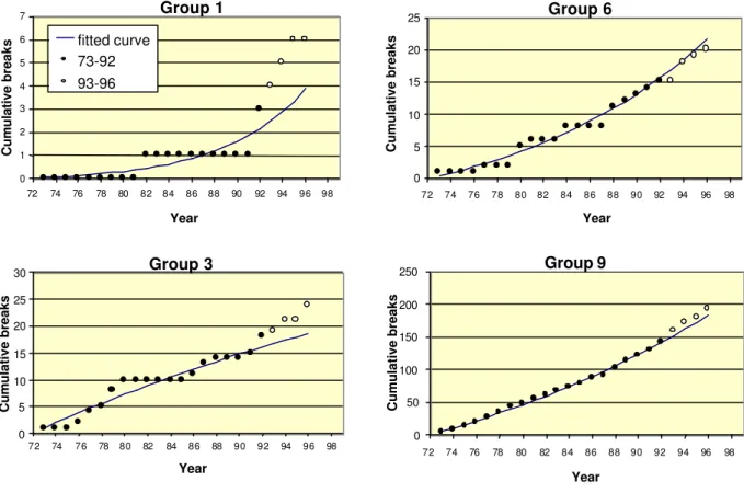
Figure 3. Time-exponential breakage patterns derived for homogeneous groups of pipes (same vintage, same soil type, etc.) in a water utility. The curves were derived using 20 years of data and their ability to predict breaks in the subsequent four years was examined (after Kleiner and Rajani 1999).
Mavin (1996) compared the time-exponential model to a time-power model depicted in equation (3) by applying both to filtered data obtained from three Australian water utilities
e t a
n = ß (3)
where n = number of breaks at time t; t = age of pipe; ε = random error term; α,β = coefficients estimated from regression analysis. He found that the performance of the two models in predicting water main breaks was comparable.
Group 1 0 1 2 3 4 5 6 7 72 74 76 78 80 82 84 86 88 90 92 94 96 98 ro Year Cumulative breaks Group 3 0 5 10 15 20 25 30 72 74 76 78 80 82 84 86 88 90 92 94 96 98 Year Cumulative breaks Year Group 6 0 5 10 15 20 25 72 74 76 78 80 82 84 86 88 90 92 94 96 98 Cumulative breaks Group 9 0 50 100 150 200 250 72 74 76 78 80 82 84 86 88 90 92 94 96 98 Year Cumulative breaks fitted curve 73-92 93-96
Clark et al. (1982) reported only moderate “goodness of fit” with r2 equal to 0.23 and 0.47 for the linear and exponential expressions, respectively. The model proposed by Clark et al. (1982) was the first reported attempt to explicitly account for several factors that were potential contributors to pipe breakage rate and to consider two distinctly different deterioration stages in the life of a water main. The linear equation (Table 1) implied that the covariates acted on the time to first breakage independently and additively. The low r2 value corresponding to the linear equation could suggest that this assumption may be incorrect and that the factors affecting pipe deterioration act jointly rather than independently. The low r2 value could also indicate that other factors affecting time to first break were present, but were not considered in the equation. The exponential equation (Table 2) is similar to other time-exponential models described above and considers the breakage rate primarily as an exponential function of time since the first break. Other covariates are assumed to act multiplicatively on the breakage rate. It should be noted that
the covariates expressing corrosivity effects are power functions. The moderate r2 value
corresponding to the exponential equation suggests that more research is required to determine the suitability of this model. The authors did not provide information as to the relative contribution of each covariate to the total r2. It is possible that the accuracy of the model could be improved if other types of data were available. The authors also did not indicate whether both equations had been applied to a holdout sample (sample of water mains that was “held out” for validation purposes and thus was not included in the data set to perform the regression analysis). Validation with a holdout sample would have provided more convincing evidence as to the predictive power of the model. Although this model has been referenced extensively, no documented reference is available to indicate if its use has been repeated elsewhere.
The economic analysis depicted in equation (2) neglects the cost of breakage repair after pipe replacement. This shortcoming may introduce inaccuracies especially when low discount rates are used, when older pipes are analysed and where the optimal (minimum cost) replacement times are in the near future. In an appendix to their paper Shamir and Howard (1979) proposed a method for accounting for breakage repair costs in replacement pipes, using perpetual replacement cycles (assumed identical) to infinity. However, in their formulation they assumed that the optimal duration of a replacement cycle is always the same whether calculated for a single or multiple cycles. This assumption may not always be valid and can thus bias the
calculated costs of perpetual replacement cycles. Kleiner (1996) and Kleiner et al. (1998) remedied this by re-deriving the economic analysis for infinite cycles in perpetuity.
It should be noted that, with the exception of Clark et al. (1982) all the models described above deal implicitly with only the wear-out phase of the bathtub curve (Figure 2). Thus, if historical failure records do include “burn-in” breaks, these (strictly speaking) should not be considered in the regression. The “time to first break” of the Clark et al. (1982) model could be viewed as an implicit consideration of the second phase in the bathtub curve.
Time-linear models
Model description. Kettler and Goulter (1985) suggested a linear relationship between pipe breaks and age (Table 2). Based on a relatively constant sample of pipes installed within a 10-year period in Winnipeg, Manitoba, they found a moderate correlation (r2 of 0.563 and 0.103 for asbestos cement and cast iron pipes, respectively) between the annual breakage rate and the pipe
age. In the same analysis, r2 increased to 0.884 and 0.672 when one outlier (a winter with an
exceptionally low breakage rate) was eliminated. Linear regression on joint failure analysis of cast iron mains found that r2 was a moderate 0.240, which increased to 0.81 without the data for outlier winter (Figure 4).
Another interesting observation was that the increase in the breakage rate of asbestos cement pipes with age was predominantly due to circular cracks. The increase in breakage rate of cast iron pipes was predominantly related to corrosion while the circular breakage rate decreased with age. Furthermore, they found a strong negative linear correlation between pipe diameter and breakage rate, indicating that larger pipes break less frequently than smaller pipes. Using six years of data from Winnipeg, they performed a weighted linear regression in which pipes with breakage rates that were more consistent (had less variation) over the six years were assigned more weight. For the available data of pipes with diameters 100 mm through 300 mm they obtained a negatively sloped line with r = –0.96. Others (e.g., Walski and Wade 1987) too have reported this observation.
Table 1. Deterministic time-exponential models.
Reference Model Notation Data requirements
Shamir and Howard (1979) ) ( 0) ( ) (t N t eAt g
N = ⋅ + t = time elapsed (from present) in years
N(t) = No. breaks per unit length per year (km-1 year-1)
N(to) = N(t) at the year of installation of the g= age of the pipe at the present time
A = coefficient of breakage rate growth (year-1)
Pipe length, installation date and breakage history; formation of homogenous groups essential according to criteria like pipe type, diameter, soil type, break type, overburden characteristics, etc.
Walski and Pelliccia (1982) ) ( 0 2 1 ( ) ) (t C C N t eAt g
N = ⋅ ⋅ ⋅ + C1 = ratio between {break frequency for
(pit/sandspun) cast iron with (no/one or more) previous breaks} and {overall break frequency for (pit/sandspun) cast iron}
C2 = ratio between {break frequency for pit cast pipes
500 mm diameter} and {overall break frequency for pit cast pipes}
Same data as for Shamir and Howard (1979) plus information on the method of pipe casting and pipe diameter. Clark et al. (1982) T x LH x RES x I x P x D x x NY 7 6 5 4 3 2 1 + + + + + + = 7 6 5 4 3 2 1 y y DEV y PRD y T y t y SH SL e e e e y REP ⋅ ⋅ ⋅ ⋅ ⋅ ⋅ = xi,yI = regression parameters,
NY = number of years from installation to first repair,
D = diameter of pipe,
P = absolute pressure within a pipe,
I = % of pipe overlain by industrial development,
RES = % of pipe overlain by residential development,
LH = length of pipe in highly corrosive soil,
T = pipe type (1 = metallic, 0 = reinforced concrete),
REP = number of repairs,
PRD = pressure differential,
t = age of pipe from first break,
DEV = % of pipe length in low and moderately corrosive soil,
SL = surface area of pipe in low corrosivity soil,
SH = surface area of pipe in highly corrosive soil
Time of installation, breakage history, type and diameter of the pipe, as well as information about operating pressures, soil corrosivity and zoning composition of area overlaying pipe. Additional types of data such as the type of breaks and pipe vintage required to enhance model.
Critique. The application of this model is simple and straight forward, similar to the two-parameter exponential model of Shamir and Howard (1979). All the qualifiers made with regard to the critique of the two-parameter exponential model on the requirement to partition data into homogeneous groups in order to implicitly consider additional variates are equally applicable to this time-linear model. The authors did not report an attempt to validate the model by applying it to a holdout sample.
Figure 4. Time-linear breakage patterns derived for cast iron pipes with bolted and universal joints installed from 1950 to 1959 in the City of Winnipeg. Winter 23 appears to be an outlier (after Kettler and Goulter 1985).
Model description. McMullen (1982) reported on a regression model that was applied to the water distribution system of Des Moines, Iowa. The investigating team concluded that corrosion was a major factor in water main failures since they observed that 94% of pipe failures occurred in soils with saturated resistivities of less than 2,000 ohm-cm. They examined several models and the one that performed the best is given in Table 2.
The coefficient of determination (r2) for this regression model was a low/moderate value of
0.375. It can be seen that the soil resistivity appears to be the most dominant factor, reducing the expected age by 28 years for every 1,000 ohm-cm reduction.
Critique. McMullen’s (1982) model predicts only the time to the first break of a pipe and
Total breaks
150 200 250
15 20 25
Age (winter seasons after installation) full set
implicitly addressing the first and second phases in the bathtub curve of Figure 2. The r2 value, although better than that of the linear equation of Clark et al. (1982), is not high enough to be considered a robust prediction. The usage of a linear function, which implies that these three covariates act on the time to first failure independently and additively, may be the source of some of the inaccuracy. The dominance of the soil electrical resistivity may on one hand raise a speculation that incorporating it into the model of Clark et al. (1982) might actually improve it. On the other hand one cannot help but wonder whether the electrical resistivity of the soil remains constant over the time period (10+ years) from installation to pipe first break, given activities such as road salting, acid rain, etc.
Model description. Jacobs and Karney (1994) in consideration of the clustering phenomenon in pipe breaks that was observed in Winnipeg (Goulter and Kazemi 1988; Goulter, Davidson and Jacobs 1993) defined independent breaks as breaks that occur more than 90 days after and/or more that 20 m from a previous break. By their definition, an independent break is often the first in a cluster of breaks.
They applied a linear regression to 390 km of 150 mm (6”) cast iron water mains with about 3,550 breakage events recorded in Winnipeg. They divided the water mains into three age groups (0-18, 19-30, and >30 years) to obtain relatively homogeneous groups of water mains, and applied the equation provided in Table 2.
Initially they applied this regression equation to all the recorded breaks and obtained coefficients of determination ranging from r2 = 0.704 to 0.937 for the three age groups. A high correlation means that pipe breaks were uniformly distributed along the pipe. A subsequent application of equation (Table 2) to the independent breaks rather than to all breaks increased r2 values of 0.957 to 0.969, which confirmed their hypothesis that independent breaks were uniformly distributed along the length of the water mains. The addition of pipe age into the regression model improved the predictive power of the model marginally for relatively new pipes, and significantly for old pipes. The authors attributed this correlation with age to different manufacturing, installation and operation practices that were typical of different age groups of pipes. The authors further observed that these differences could be classified geographically and that the age (or rather the “vintage”) of a pipe may be a convenient surrogate measure which may be gathered and managed in a Geographic Information System (GIS).
Table 2. Deterministic time-linear models.
Reference Model Notation Data requirements
Kettler and
Goulter (1985) N =k0Age
N = number of breaks per year
k0 = regression parameter
Same data as for Shamir and Howard (1979).
McMullen
(1982) Age=65.78+0.028SR−6.338pH−0.049rd
Age = age of pipe at first break (years)
SR = saturated soil resistivity (ohm-cm)
pH = soil pH
rd = redox potential (millivolts)
Data required typically not available; sporadic data collection not expensive, however, continuous and extensive data collection program is costly; continuous monitoring of soil properties is
important where ground water conditions have not reached steady state or are seasonally dependent. Jacobs and
Karney (1994) P=a0 +a1Length+a2Age
P = reciprocal of the probability of a day with no breaks
a0,a1,a2 = regression coefficients
Pipe length, age and breakage history; more data enables formation of homogenous groups.
Critique. Jacobs and Karney (1994) provide useful insight into the distribution of so-called independent breaks along the water mains. Their results indicate that the independent breaks are distributed more uniformly than the total breaks along the pipes, especially in younger pipes. It is not clear whether this phenomenon is general or unique to the distribution system in Winnipeg. The authors used random samples comprised 5, 10, 15, …100 pipe links with varied length but do not provide information on the age of each sample, since each sample is likely to consist of pipes of various ages.
At first glance it is not obvious that this model is a real time-linear model. Since the length of water mains in a utility is relatively constant, one can divide the equation (Table 2, Jacobs and
Karney 1994) by the length variable and convert all the parameters to units of [length]-1. The
model reduces to a two parameter, single variate (age) linear equation, which is precisely a time-linear model with an implicit assumption of uniform (time-linear) distribution of breaks along pipe length. According to Jacobs and Karney (1994) this implicit assumption is justified when the regression is applied to independent breaks only.
With the exception of the McMullen (1982) model, the linear models, like the time-exponential and the time-power models, implicitly consider only the wear-out phase in the bathtub curve.
Probabilistic Multi-variate Models Proportional hazards models
The proportional hazards model is a general failure prediction model proposed by Cox (1972), which takes the general form
Z bT e t h Z t h( , )= 0() (4)
where t = time; h(t, Z) = hazard function, which is the instantaneous rate of failure (probability of failure at time t+∆t given survival to time t); h0(t) = arbitrary baseline hazard function; Z = vector of covariates acting multiplicatively on the hazard function; b = vector of coefficients to be estimated by regression from available data.
Figure 5. Proportional hazards model (after Andreou et al. 1987b) for a 100 m long pipe with no previous breaks, that was installed after 1950. The base hazard describes this pipe operating at 30 m of pressure and 20% of its length lies under a low
development area. If it reached the age of, say, 70 years without breaking, its
instantaneous probability of breakage (say breakage in the next year, is about 1.5%. The probability of this pipe to reach age 70 without a break is about 63%. The thin full line describes the same pipe when 80% of its length is under a low development area. The hazard and the survival change accordingly. The dashed line describes the same pipe operating at 60 m pressure.
0 0.02 0.04 0.06 0.08 0 20 40 60 80 100 120 Pipe age Break hazard Base hazard +60% low development +30 m pressure 0 0.2 0.4 0.6 0.8 1 0 20 40 60 80 100 120 Pipe age
The concept of the proportional hazards is demonstrated in Figure 5. The baseline hazard
function h0(t) can be interpreted as a time-dependent ageing component, while the covariates
represent environmental and operational stress factors that act on the water main to increase or reduce its failure hazard. Further, the data can be partitioned (or “stratified”) with respect to a covariate if it is judged to act on the hazard function in a non-multiplicative manner, and a different baseline hazard function can be derived if necessary. A priori knowledge of the baseline hazard function is not required in order to estimate the elements in vector b.
Marks et al. (1985) was first to propose the usage of the proportional hazards model to predict water main breaks by computing the probability of the time duration between consecutive breaks. Multiple regression techniques were used to determine covariates Z that could affect pipe breakage rates. The most significant covariates found by Marks et al. (1985) are listed in Table 3.
The baseline hazard function h0(t) was approximated by a second degree polynomial (Table 3),
similar to the bathtub effect, in which the hazard decreases initially then increases. It should be reiterated, however, that the parabolic h0(t) here does not correspond to the bathtub depicting the life cycle of a pipe (ROCOF) illustrated in Figure 2. Rather it depicts the instantaneous probability of the next break after installation (for a pipe with no previous breaks) or after the last break (for a pipe with previous breaks). The parabolic h0(t) proposed by Marks et al. (1985), had a minimum at t = 28 years (Figure 5), which means that according to their observations, the probability of a break decreases as the pipe “matures” after installation or after the previous break. Then, after about 28 years the pipe begins (or resumes in the case of a pipe with previous breaks) its deterioration and the probability of the next break increases. The model was tested with two censoring schemes and appeared to have little sensitivity to left data censoring1, which is an important characteristic because most water utilities have incomplete records of pipe breakage and repair. Marks et al. (1985) provided a cost analysis for determining optimal timing for pipe replacement based on minimising the expected costs that are associated with a pipe.
Andreou et al. (1987a, 1987b) and Marks et al. (1987) further developed the proportional hazards model to include a two stage pipe failure process. The early stage was characterised by fewer breaks and was represented by the proportional hazards model, while the late stages, with multiple and frequent breaks were represented by a Poisson type model. They observed that
1 Left censoring, in this context, means incomplete data due to early breakage records that
pipes rarely broke soon after they were installed, and that each additional break typically
shortened the time to the next break (which meant that the h0(t) became tighter parabolas with
minima increasingly smaller than 28 years). After the third break, the breakage rate of the pipes seemed to be constant (and frequent) regardless of the number of previous breaks and the pipe age. Consequently, the third break was selected as the cut-off point between the two stages of failure. A Poisson process was assumed for the late stage where the average breakage rate appeared constant over time and thus the inter-breakage times were exponentially distributed with an average failure rate estimated by ? = ebTZ. Since the hazard function for the exponential distribution is constant and equal to the average failure rate, it follows that the hazard h for the late stage is expressed by
Z bT e
h = λ = (5)
which has the same form as the early stage, as in equation (5), except the time dependent component h0(t) is transformed into a constant. Andreou et al. (1987b) reported a moderately low r2= 0.34 in the prediction in the late stage, when the cut-off between the early and late stage was 3 breaks. When the cut-off was taken as 6 breaks it increased to r2= 0.46.
Eisenbeis (1994) and Brémond (1997) reported the application of the proportional hazards model to water distribution networks in France, while Lei (1997) reported their in Norway. In France the Weibull probability baseline hazard function for the water main failure (Table 3) was used. It was not clear if a two-stage failure process model was used as in Andreou et al. (1987a). Eisenbeis (1994) and Brémond (1997) reported good predictions of the aggregate number of breaks in an eleven-year period in Bordeaux, France, based on failure data from the preceding 33 years. Lei (1997) found that pipe material was a stratification criterion rather than an explanatory variate, implying that the underlying ageing processes are different for various pipe materials. The report did not provide any indication as to the quality of predictions and it appears that the second stage was not implemented using a Poisson process as described by Andreou et al. (1987a).
Li and Haims (1992a, 1992b) formulated a two-stage decision-making process based on Andreou et al.’s proportional hazards and Poisson model. In the first stage a semi-Markovian model was applied to individual water mains to determine the optimal repair/replace decision at
stage uses a multilevel decomposition approach to optimally distribute available funds among the distribution network components, so as to maximise overall system availability. The authors acknowledged that the data required to quantify all the necessary transition probabilities may be beyond what is available in most water utilities. The model also did not consider network hydraulics.
Critique. The proportional hazards model appeals to many researchers because of its versatility and robust theoretical basis. The multiplicative effect that the covariates have on the hazard function is intuitively appealing. The ability to compare various strata in the water main population is very useful, as is the relative insensitivity to left-censored data and the ability to consider right-censored data. The inclusion of several variates in a single analysis reduces significantly the amount of pre-grouping that is required by simple, two or three parameter models. This grouping requirement is not altogether eliminated and careful analysis is required to identify groups of pipes that may differ in their underlying ageing process. Further, the underlying assumption that environmental and operational stresses act to increase or decrease the failure hazard of all types of pipes in the same proportion may sometimes be invalid. For instance, soil resistivity has a significant affect on unprotected cast iron pipes, but may have a lesser affect on coated or cathodically protected pipes. If these two categories are not stratified (or partitioned) in the analysis, the differences may reduce the accuracy of the results.
The constant hazard function in the second phase of Andreou et al.’s (1987a and b) model implies that after their third break, pipes no longer age, as their failure hazard remains constant (see alternative B to the wear-out phase in the bathtub curve in Table 2). This observation was corroborated by others (e.g., Herz 1996) but at the same time it contradicts the physical realm of ageing pipes, especially where corrosion exists. It is possible that there is a practical limiting state for the ageing of a given pipe. This limiting state may be determined by how frequently it is practical to fix its breaks before actually replacing it. It appears that this limiting state will usually be reached at a stage that is much later than three or even six breaks. More research with larger based data sets may be required to resolve this point.
The proportional hazards model is quite powerful but it also requires significant technical expertise to apply. As was stated earlier, careful examination of the data is required in order to identify the covariates with the best predicting ability, as well as those which are required for data stratification.
It should be noted that in the proportional hazards model with a parabolic h0(t), the first parabola, depicting the time to first failure could be viewed as implicitly corresponding to the first and second (burn-in and in-usage) phases of the bathtub curve in Figure 2. Subsequent breaks would thus correspond to the wear-out phase, and the constant breakage rate (modelled by the Poisson process) corresponds to alternative B of the wear-out phase in Figure 2.
Data requirements. The proportional hazards model can be applied with any level of data availability. Of course, the more data on the covariates that may affect pipe failure hazards, the more beneficial is its usage, and predictions could even be extended to the individual pipe level. Significant covariates may vary from one utility to the next, depending on prevailing environmental and operational conditions and on the types of pipes used. It appears that currently, lack of data in most utilities would limit the potential benefits of this model.
Accelerated lifetime models
Lei (1997) examined an accelerated lifetime model of the form provided in Table 3. The essence of the accelerated lifetime models is that time to next failure expands or contracts relative to that at x = 0, where x is defined as a vector of explanatory variables (see broad definition in Table 3). Lei (1997) applied both proportional hazards and accelerated lifetime
models to the distribution system of Trondheim, Norway. The explanatory variates
x
were agegroups, pipe size groups and length of pipe. The report did not note whether the model was validated or comment on the quality of the predictions. No significant difference was found between the results of the two models, which should not come as surprise since it can be shown that an accelerated lifetime model translates into proportional hazards when Z has a Weibull distribution (Cox and Oakes 1984).
Eisenbeis et al. (1999) applied the accelerated lifetime model (Table 3) to three water distribution systems in Norway and France. They assumed that Z followed the extreme value distribution for minima (or the Gumbel distribution). The covariates used for each system varied according to local conditions. Using the previous number of breaks as a covariate complicated the application of the method necessitating the use of Monte-Carlo simulation for the prediction of the number of failures at a desired time-horizon. The authors reported good predictions using this method but did not provide any details to demonstrate them.
Critique. The accelerated lifetime model can be viewed as analogous to the proportional hazards model. It differs from the proportional hazards model in that the covariates act on the time to failure, whereas failure hazard is affected in the proportional hazards model. In both models the effects are multiplicative and covariates that are thought to act in a non-multiplicative manner would require data partitioning. Like the proportional hazards, the accelerated life model is quite versatile as long as the data are available, and requires significant technical expertise to apply it effectively. The manner with which the accelerated life model relates to the bathtub life cycle curve (Figure 2) can be determined only after inter breakage times are obtained from a specific data set. For example, if results show that the time to first break is shorter than the time between the first and second break and the time between higher order breaks becomes increasingly shorter, that would indicate an explicit depiction of all three phases of the bathtub curve.
Time-dependent Poisson model
Model description. Constantine and Darroch (1993) and Constantine et al. (1996) proposed a model where pipe breakage follows a Poisson process in which the mean breakage rate depends on pipe age as is depicted in Table 3. This process is also known as a Weibull process, because the resulting cumulative distribution in this process is precisely equivalent to the Weibull cumulative distribution function. The parameter ß (shape parameter) was considered by the authors to be constant for a homogeneous group of failures (e.g. failures that are attributed to corrosion only), whereas ? (scale parameter) was a function of some operational and environmental covariates (Table 3).
Miller (1993) applied this model to a data set containing about 1,150 asbestos cement and cement-lined cast iron water mains, with about 2,600 recorded breakage events in Melbourne, Australia. This set was reduced to only those mains that had at least five breaks. It was assumed that for those pipes the principal cause of failure was corrosion. The covariates that were found to contribute to θ were mean static pressure, overhead traffic conditions, pipe diameter and soil type. The model could explain 68% of the variation in the breakage rates. In some pipes the differences between the expected and the actual number of breaks were markedly large, prompting the speculation that the underlying cause of some of the failures had not been corrosion which meant that the β was inappropriate for all the pipes. The author did not report
any attempt to fit the model into a holdout data set, thus testing its ability to predict failures that were not part of the data used for parameter derivation.
Mavin (1996) used the time-dependent Poisson model of Constantine and Darroch (1993) to filter out of a given data set those water main breaks that were not likely to be the result of a natural deterioration process. He calculated the probability of occurrence of any two successive failures in a water main. The covariates used were pipe diameter, material, traffic level and soil type, and the coefficients were given without an explanation as to how and where these coefficients had been derived. He proposed the following rules:
• When two successive breaks occurred in spite of a very low probability (1% was suggested)
and also occurred within a small distance (5 m was suggested) from each other – the second break was assumed a “bad repair” and was thus filtered out of the data. This is similar to the spatial breaks clusters concept introduced by Goulter et al. (1993) and Jacobs and Karney (1994).
• When a break occurred less than two days after the previous break – the second break was
assumed to be related to careless re-pressurisation of the system after the repair of the previous one, and was thus filtered out of the data set.
• When two successive breaks occurred in spite of a very low probability, and these
occurrences took place in a period of industrial tension in the utility, or during a holiday period in which overtime rates are very high – these breaks could be due to intentional damage and may thus be filtered out.
• Two successive breaks occurring in spite of an extremely low probability (e.g., 0.1%) could
be attributed to faulty operational procedures or accidental damage and may thus be filtered out.
Table 3. Probabilistic multi-variate models - proportional hazards and accelerated life.
Reference Model Notation Explanatory variables (data)
Proportional hazards Marks et al. (1985) Z bT e t h Z t h( , )= 0() 2 7 5 4 0(t) 210 10
t
210t
h = ⋅ − − − + ⋅ −T = time to next break
h(t, Z) = hazard function
h0(t) = baseline hazard function
Z = vector of covariates
b = vector of coefficients to be estimated by maximum likelihood
• natural log of pipe length
• operating pressure
• percentage of low land development
• pipe “vintage” (or period of installation)
• pipe age at second (or higher) break rate
• number of previous breaks in pipe
• soil corrosivity Andreou et al.
(1987a, 1987b) Marks et al. (1987)
Early stage: same as Marks et al. (1985) described above
Late stage: h = λ =ebTZ
h = hazard (constant at the late stage) Same as above
Proportional hazards Brémond (1997) Z bT e t h Z t h( , )= 0() 1 0( ) ( ) − =λβ λt β t h
t = time to (next) failure
h(t) = hazard function
?, ß, = scale and shape parameters (respectively) of the Weibull distribution
• number of previous breaks
• pipe diameter • ground conditions • traffic loading Time dependent Poisson model Constantine and Darroch (1993), Miller (1993); Constantine et al. (1996) β θ = t t H( ) Z eα θ θ = 0 t = pipe age
H(t) = mean number of failures per unit length at age t
?, ß, = scale and shape parameters, respectively
?0 = baseline value
a = vector of coefficients to be estimated by regression;
Z = a vector of covariates affecting breakage rate.
• mean static pressure
• overhead traffic conditions
• pipe diameter
Table 3. (Continued).
Reference Model Notation Explanatory variables (data)
Accelerated life Lei (1997) µ σ β σ β µ T x T e Z f T Z x T ) , , ( ) ln( = ⇒ + +
= T = time to (next) failure
x = vector of explanatory variables
Z = random variable distributed as Weibull
σ = parameter to be estimated by maximum likelihood
ß = vector of parameters estimated by max likelihood
• pipe age group
• pipe size
• pipe length
• pipe material was taken as stratification criterion
Accelerated life
Eisenbeis et al. (1999)
Same as Lei (1997) above Z = random variable distributed as Gumbel (extreme distribution for minima)
• log of pipe length
• pipe diameter
• pipe material
• traffic loading
• soil acidity
• soil humidity
• number of previous breaks was taken both as a covariate and as a stratification variate
Critique. The time-dependent Poisson model represents the pipe breakage rate as a power function of time or pipe age where the accelerated time equation can be rewritten as
β
θ t t
H( )= ' (6)
The scale parameter θ’ is modified by environmental and operational covariates, while the power parameter β is said to be unique to the type of failure (e.g., corrosion-related, longitudinal split,
etc.). The function θ0’tβ is thus similar conceptually to the base hazard function in the
proportional hazards model. Change in β is analogous to stratification in the proportional hazards model, and the scale parameter which is modified multiplicatively by a vector of covariates, is analogous to the failure hazard modifiers in the proportional hazards model. The potential strengths and caveats inherent in this model are similar to those mentioned for the proportional hazards model except that it appears that this time-dependent Poisson model is less able to deal with left censored data. The manner with which this model has been applied by Miller (1993), using only pipes that had at least five breaks, raises the question of how to deal with those pipes that had fewer breaks. It may be possible to group together adjacent pipes provided they are similar with respect to the covariates used for prediction. There have been no reports about applying this model to other distribution networks. This model, which is essentially a time-power model, corresponds implicitly only to the wear-out phase in the bathtub curve.
Probabilistic Single-variate Group-Processing Models Cohort survival models
Model description. Herz (1996) proposed a lifetime probability distribution density function based on the principles that had originally been applied to population age classes or cohorts. The probability density f(t), hazard h(t) and survival S(t) functions are given in Table 4. The parameter c, resistance time, in fact corresponds to the burn-in phase of the bathtub curve in Table 2. It can be shown that the hazard function approaches the constant value b asymptotically as the age t increases, and the Hertz distribution approaches an exponential distribution. As previously noted a hazard function whose value remains constant corresponds to no ageing, which concurs with the observations of Andreou et al. (1987a) and thus corresponds to the alternative B of the wear-out phase of the bathtub curve (Figure 2). The observed constant hazard refers to pipe breakage in the context of Andreou et al.’s model while Herz refers to pipe “death” or pipe replacement. When a = 0 the distribution becomes an exponential function shifted to the
right by c, and the hazard function again becomes a constant which implies no ageing (hence the naming of parameter a as the ageing parameter). Herz (1996) proposed to apply the model to groups (cohorts) of pipes that are homogeneous with respect to their material type and environmental/operational stress class. The estimation of parameters a, b and c was done using water utility data, where historically, the time that a pipe had been replaced was considered to be the time of its “death”.
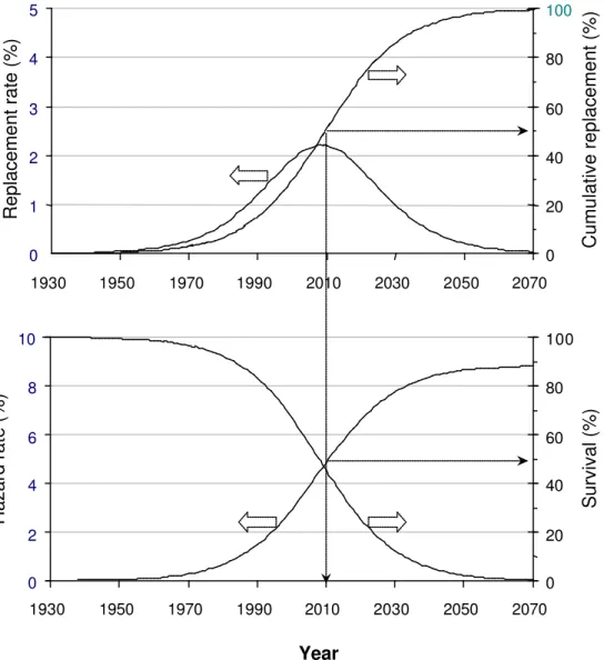
Figure 6. The Herz model applied to a homogeneous group of pit-cast iron water mains installed between 1900 and 1929, in Clay soil. The pipe “time of death” was defined as the end of its economical life. The plot indicates a median survival of 50% (i.e. 50%) of the pipes in the group would likely have to be replaced by the year 2010. Note also the hazard rate which tends to a constant of about 8% as the water mains
0 2 4 6 8 1930 1950 1970 1990 2010 2030 2050 2070 Hazard rate (%) 0 20 40 60 80 100 Survival (%) 10 0 1 2 3 4 5 1930 1950 1970 1990 2010 2030 2050 2070 Replacement rate (%) 0 20 40 60 80 100 Cumulative replacement (%) Year
Deb et al. (1998) applied the cohort survival model (“KANEW”) to one British and four American water utilities. A Delphi process was used to estimate the three parameters for the model when sufficient historical “pipe death” data were not available.
Herz (1998) presented a case study and a framework to use the cohort model in the long-term planning of water mains renewal. In this framework the planner generates various scenarios that include different rates of pipe replacement and/or rehabilitation, in order to find the most suitable strategy. Appropriate assumptions have to be made on the performance and life expectancy of the replacement pipes and/or rehabilitation technologies. These scenarios can include, in addition to ageing parameters, expected failure frequencies and economic data such as direct and (if available) indirect cost of pipe failure, rehabilitation and replacement costs, etc.
Critique. The cohort survival model can be a useful tool for evaluating the future financial needs of a water distribution system. It may provide useful insight into the long-term planning of water main renewal budgets. The model can only deal with relatively large groups of water mains and is not suitable for prioritising individual pipes for rehabilitation. The assumption that a pipe actually reached the end of its useful life when it was replaced by the utility introduces a weakness in the application of the model because the decision to replace a pipe does not always indicate that the pipe had indeed reached the end of its useful life. Historical pipe replacement decisions often reflect political choices (e.g., allocation of resources) or perceptions rather then best technical judgement. Kleiner and Rajani (1999) proposed an alternative approach. They posited that the useful life of a pipe is an economic outcome of its deterioration rate, thus suggested that the pipe “death” coincided with the optimal time of its replacement. They partitioned the pipe inventory into relatively homogeneous groups and, for each group established the optimal age of pipe replacement, based on projected breakage rates and cost data. They then derived the appropriate parameters and replacement rates for the respective groups, as is illustrated in Figure 6.
Bayesian diagnostic model
Model description. Kulkarni et al. (1986) developed the Cast Iron Maintenance Optimisation System (CIMOS) for the Gas Research Institute to identify failure-prone segments of gas pipes and to determine the optimal time for their replacement. They identified two groups of pipe characteristics, static (e.g., diameter, length, soil type, etc.) and dynamic (e.g., cumulative
number of breaks, age, etc.). The basic premise of the model was that the probability of failure (break or leak) in a pipe segment can be related to three factors: (1) system-wide probability of failure Pf, (2) probability of observing specified characteristics on a segment that failed Pc/f, and, (3) the probability of observing the same characteristics on a segment that has not failed Pc/nf. According to Bayes theorem
[
]
(1 ) . Prob / / / stics characteri specified failure f nf C f f c f f c P P P P P P − + ⋅ ⋅ = (7)If the Prob.[failurespecified characteristics] is close in value to Pf (= system-wide
probability of failure), then this particular set of characteristics has little diagnostic capability. If the value is significantly larger or smaller than Pf, then the presence of this set of characteristics can “explain” a relatively high (or low) breakage rate. The system-wide average probability of failure/segment/year is calculated
∑
∑
= = = N i N i f i i P 1 1 year in segments of number Total year in break one least at with segments of number Total (8)where N = total number of years accounted for in the database.
The probability of observing specified characteristics in a pipe that has failed is
∑
∑
= = = N i N i j f c i i c P j 1 1 year in failure one least at show that segments of number Total year in break one least at show that stics characteri with segments of number Total (9)where Cj = a set of characteristics, also called a condition state.
Condition states can be defined by combinations of individual characteristics. For example, a condition state of a pipe segment can be age 50 year, 150 mm (6”) diameter, 100 m long in clay soil, etc. After identifying condition states Cj for which P[f/Cj] is significantly different than Pf,
one can calculate the expected number of failures in one year on a given segment E[n/Cj]
] state condition in failure one least at th segment wi a on year one in failures of number expected year one in failure one least at [ ] Prob[ ] [ j C j j C C n E = ⋅ (10)
The first term in the right hand side of equation (10) is calculated using equation (7). The second term depends on the segment length. This dependence can be estimated by an appropriate regression analysis of number of failures versus segment length.
As previously mentioned, this procedure was developed for the gas industry, where the consequences of failure can be grave. Thus, it is necessary to estimate the probability of various consequences given that a pipe failure had occurred. The issue of consequence of failure has not yet been addressed rigorously in the water industry, while pertinent data is scarce and awareness is generally low.
The authors validated the procedure on two sets of data and reported good agreement between the predicted and observed failure rates. A decision procedure was also developed for optimising segment replacement strategies. This procedure is based on a dynamic process in which a decision has to be made at the end of every year as to whether it is cheaper to replace the pipe now, or postpone a decision to the next year while repairing the failures this year as they occur. This can be summed up by the general recursive formulation
+ − + =
∫
F m R c x V x dF x c c x V ; ( ) ( ') ( ') 1 min ) ( 0 α α (11)where V(x) = optimal decision (minimum cost) for a given segment; x = expected number of failures in the segment at the current year; x’ = expected number of failures in the segment at the
next year; cR = segment replacement cost; cm = annual expected maintenance cost of the new
(replaced) segment; α = discounting factor, cm/(1-α) = discounted maintenance cost; Σcm = discounted maintenance cost from present to infinity; co(x) = expected cost of failure repair at the current year; dF(x’) = probability distribution of x’. The CIMOS was subsequently developed by Woodward-Clyde Consultants into a full-fledged computer application for managing the maintenance and planning of gas lines.
Critique. The Bayesian diagnostic model is based on some simple and robust mathematical principles in which the mains are partitioned into homogeneous groups with respect to some criteria (condition states), and the failure ratios in these groups are systematically compared and evaluated. The model is “flat” with respect to time. It does not consider the time of breakage occurrence, just the cumulative number of breaks to the time of analysis. It implicitly then assumes that the ratios of cumulative number of breaks between the various condition states will
be the same in the next year. The model, therefore, cannot predict the number of breaks over time, rather it indicates the probability of failure, or the expected number of failures in the next time period. The model can therefore be used for analysing repair/replacement decisions in the next year rather than for formulating long-term replacement strategies. The model assumes that breaks are linearly related to pipe length for a given condition state, an assumption that has been challenged by others. The authors do not provide any information as to the sensitivity of the model to left-censored data. It would seem that since the model deals mainly with the cumulative number of breaks, left censored data would have relatively little affect, but this needs to be verified.
Data requirements. For a simple analysis, only pipe lengths and breakage history are needed. A detailed analysis requires partitioning the mains into an extensive list of condition states. The appropriate criteria for these condition states are required, which is equivalent to the grouping criteria mentioned previously in the application of other models.
Break history as a semi-Markov process
Model description. Gustafson and Clancy (1999a) modelled the breakage history of water mains as a semi-Markov process in which each break order (e.g., 1st, 2nd ,3rd break, etc.) is considered a “state” in the process and the inter-break time ti is considered the “holding time” between state (i-1) and state i. The semi-Markov process implies that the time to the next break ti is completely independent of the times between previous breaks (tj, j<I), rather it depends solely on the break order i. The time from installation to the first break t1 was modelled as a three parameter gamma distribution while the subsequent inter-break times (ti, i>1) were modelled as exponential distributions with parameters 1/λi. The λi are in fact the mean of their respective exponential distributions. The breaks were found to decrease as i increased, which means that the higher the number of previous breaks in a pipe, the shorter the expected time to the next break. The inventory of pipes in Saskatoon, Saskatchewan, was partitioned into thick wall, medium wall and thin wall water mains, and this concept was applied to the three groups of pipes. It was found that the mean time to first break was 96, 44 and 34 years for the thick, medium and thin wall pipes respectively. The expected times to second, and higher breaks became increasingly smaller for all three groups, until they almost converged and became approximately constant
(2.1, 1.9 and 1.4 years respectively) from the 9th-10th break. This apparent tendency towards constant breakage rate has been discussed previously.
Gustafson and Clancy (1999b) applied a Monte Carlo simulation, using the parameters they had derived for the inter-break times, to generate breakage rate predictions for the future. They obtained a prediction that the breakage rate in the five years subsequent to the analysis will increase more than 50% per year. This outcome was judged an unreasonably over-prediction that was likely the result of deterioration mechanisms that had changed over the life of the water mains. They then used a simple Bayesian process to extract transition probabilities based only on data taken from the five years preceding the analysis (reasoning that deterioration processes are relatively constant in a five-year period and are unlikely to change in the next five-year period).
These transition probabilities were then used to re-derive λi parameters (representing mean
holding times) for the second and higher breaks. They then re-applied the results in the semi-Markov framework to predict future breakage rates of about 20% per year increase in the subsequent five years.
The authors also presented a method for using the model to determine the optimal time of replacing a water main. They used Monte Carlo simulations to generate synthetic breakage histories, based on the parameters derived earlier. The pertinent costs (e.g., breakage repair and replacement costs) were attached to the synthetic history and the pipe replacement year that would minimise the discounted stream of costs was obtained. This is similar to equation (2) except that it is applied on a synthetic data set. They used a concept of “expected economic loss” to translate the optimal replacement timing to an optimal replacement break order (i.e., after which break the pipe should be replaced to minimise total costs).
Critique. Gustafson and Clancy (1999a, 1999b) provide additional insight into the deterioration rates of water mains. Their findings are intuitively appealing and their method lends itself relatively easily to computer implementation. They developed an elaborate model to predict the inter-break times in water mains, based on historical data, but found this model inadequate for predicting future breaks. They reasoned that this inadequacy is the result of conditions that changed over the years, and thus ended up basing their predictions not on the original model but rather on a different process that used the data from only the preceding five years. If this reasoning were correct, it would imply that a semi-Markov process with stationary transition probabilities may not be appropriate because of changing conditions throughout the