A comparative test method to determine thermal resistance under field conditions

Publisher’s version / Version de l'éditeur:

Journal of Thermal Insulation and Building Envelopes, 18, OCT, pp. 163-181,

1994-10

READ THESE TERMS AND CONDITIONS CAREFULLY BEFORE USING THIS WEBSITE. https://nrc-publications.canada.ca/eng/copyright

Vous avez des questions? Nous pouvons vous aider. Pour communiquer directement avec un auteur, consultez la première page de la revue dans laquelle son article a été publié afin de trouver ses coordonnées. Si vous n’arrivez pas à les repérer, communiquez avec nous à PublicationsArchive-ArchivesPublications@nrc-cnrc.gc.ca.

Questions? Contact the NRC Publications Archive team at

PublicationsArchive-ArchivesPublications@nrc-cnrc.gc.ca. If you wish to email the authors directly, please see the first page of the publication for their contact information.

NRC Publications Archive

Archives des publications du CNRC

This publication could be one of several versions: author’s original, accepted manuscript or the publisher’s version. / La version de cette publication peut être l’une des suivantes : la version prépublication de l’auteur, la version acceptée du manuscrit ou la version de l’éditeur.

Access and use of this website and the material on it are subject to the Terms and Conditions set forth at

A comparative test method to determine thermal resistance under field

conditions

Bomberg, M. T.; Muzychka, Y. S.; Stevens, D. G.; Kumaran, M. K.

https://publications-cnrc.canada.ca/fra/droits

L’accès à ce site Web et l’utilisation de son contenu sont assujettis aux conditions présentées dans le site LISEZ CES CONDITIONS ATTENTIVEMENT AVANT D’UTILISER CE SITE WEB.

NRC Publications Record / Notice d'Archives des publications de CNRC:

http://www.nrc-cnrc.gc.ca/irc

A c om pa ra t ive t e st m e t hod t o de t e rm ine t he rm a l re sist a nc e unde r

fie ld c ondit ions

N R C C - 3 7 8 2 0

B o m b e r g , M . T . ; M u z y c h k a , Y . S . ; S t e v e n s , D . G . ;

K u m a r a n , M . K .

O c t o b e r 1 9 9 4

A version of this document is published in / Une version de ce document se trouve dans:

Journal of Thermal Insulation and Building Envelopes,

18, (OCT), pp. 163-181,

October, 1994

The material in this document is covered by the provisions of the Copyright Act, by Canadian laws, policies, regulations and international agreements. Such provisions serve to identify the information source and, in specific instances, to prohibit reproduction of materials without written permission. For more information visit http://laws.justice.gc.ca/en/showtdm/cs/C-42

Les renseignements dans ce document sont protégés par la Loi sur le droit d'auteur, par les lois, les politiques et les règlements du Canada et des accords internationaux. Ces dispositions permettent d'identifier la source de l'information et, dans certains cas, d'interdire la copie de documents sans permission écrite. Pour obtenir de plus amples renseignements : http://lois.justice.gc.ca/fr/showtdm/cs/C-42

A Comparative Test Method to

Determine Thermal Resistance

under Field Conditions

M.

T.

Y.

D. G.

AND M.

K.

National Research Council of Canada IRC-Building M-24 Ottawa, Ontario, KIA OR6 Canada

ABSTRACT: This paper presents the development and application ofa test method to determine thermal resistance of a material under transient conditions. The method consists of testing two material slabs placed in contact with one another, one of them being a reference material with known dependence of thermal conductivity and heat capacity on temperature and the other being a test specimen whose thermal proper-ties are to be determined.

Thermocouples are placed on each surface of the standard and reference materials to measure temperatures during a transient heat transport process. These tempera-tures are used as the boundary conditions in a series of calculations. First, the heat flux across the contact surface between the reference and the test specimen is calculated using a numerical algorithm to solve the heat transfer equation through the reference material. Then, imposing the requirement of heat flux continuity at the contact surface, corresponding values of thermal conductivity and heat capacity of the test specimen are calculated with an iterative technique. These calculations, done as a function of time, result in a set of thermal properties of the test specimen for the range of boundary conditions imposed during the transient process.

This method can be used under transient conditions of either laboratory or field testing. Of particular interest is its application to examine effects of aging (effect of time) and weathering (effect of time and environmental conditions) on thermally in-sulating foams. For instance, in this research, the reference and tested specimens are

*Senior Researchers at the National Research Council of Canada. **Summer Assistants at the National Research Council of Canada.

J. THERMAL'NSUL. AND8LDG. ENVS. Volume 18-October1994 163

1065-2744/94/02 0163-19 $06.00/0 ©1994 Technomic Publishing Co., Inc.

164 M. T. BOMBERG ET Al.

placed in an exposure box representing a conventional roofing assembly and the change in the thermal properties of the test specimens is determined.

KEY WORDS: heat flow, heat flux measurements, field testing, aging of foams,

field exposures, thermal resistance, R-value.

INTRODUCTION

M

usually performed with a heat flow transducer (HFT). A typical HFT is calibrated in such a manner that the thermopile output indicates the heat flux normal to the HFT surface[1].While HFT calibration relates to steady

state conditions, HFT can also be used under transient conditions ifthe

transducer is calibrated as a function of temperature and if the transducer has a response period much shorter than that of the tested system. An alternative approach is to reduce the effect of short-term responses by locating the transducers between two layers of insulation, as is done in the Roof Thermal Research Apparatus at the Oak Ridge National Laboratory [2].

While Wilkes [2] compared measured and calculated heat fluxes, Anderlind [3] applied a multiple regression analysis ofin situheat flux

mea-surements to derive information on the thelmal resistance of loose fill

in-sulation in an attic space. More detailed analysis was presented by Courville and Beck [4], who reviewed various techniques for calculating the thermal

properties of insulations from transient heat flux measurements.

The method presented in this paper employs similar ptinciples to the mul-tiple regression technique reported by Anderlind [3] and the sum of least squares technique introduced by Courville and Beck [4], but differs in details of calculations and measurements. Instead of using a small HFT, the reference material has a surface area as large as that of the test material. This eliminates the increase of heat flow at the edges of the HFT and permits us-ing a permeable reference material, viz. glass fiber insulation. Both the ther-mal conductivity and the heat capacity of the reference material must be

known as a function of temperature. The measurements required for

ap-plication of the heat flux comparator (HFC) technique involve only the

tem-peratures of the free surfaces of the test specimen and the reference material

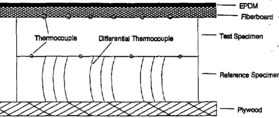
and at the interface of the two (see Figure 1). This implies that HFC

tech-nique can be used for field measurements on existing structures, for

materials forming sides of an outdoor exposure box (as in this paper), or for

laboratory measurements performed under varying environments.

A numerical algorithm developed in this work optimizes the thermal

A 'lest Method to Determine Thermal Resistance under Field Conditions 165 -EPDM - Fiberboard - Test Speelmen - - Reference Speelmen Differential ThennocaupJe ThennocoupJe

/

FIGURE1. Placement of thermocouples on surfaces of the test and the reference specimens as used in the actual field study [II}.

measured. The physical principles of the method and the numerical tech-nique are briefly described below.

APPROXIMATION OF HEAT TRANSFER THROUGH A SLAB

Fourier's heat transport equation in one dimension and the corresponding energy conservation equation are used as the axioms. Following the ap-proach of Stephenson [5] and introducing Kirchoff'sl potential function, "fJ,

(1)

where Xis the thermal conductivity, W/(m K), and T is the temperature, DC,

the axioms can be expressed as: .

aTf

q.

= --

_ox

and

O"fJ X

a

_Tf

ar = eCp' 8x2 (energy conservation equation) (3)

166

In Equations (2) and (3):

M. T.BOMBERG ET AL

qx = one dimensional heat flux (W/m2 ) Q = density of the medium (kg/m3)

Cp

=

x = distance (m)

l' = time (s)

If A can be expressed as a linear function of temperature as:

A

=

+

(4)

where Ao and {3 are the thermal conductivity at OOC and the temperature coefficient of thermal conductivity, respectively, then, ll-function is related to temperature as follows:

11 =: AoT

+

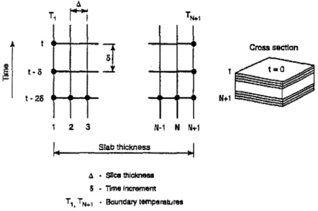
The calculations are performed with a numerical approximation of the en-ergy conservation equation, Equation (3). To derive such an approximation, both the reference and test specimens are divided into N layers, numbered so that the outer surface of each material is the £lrst position and the contact surface is (N

+

adja-ｾＱ

Ｑｾ

ｎＫｬｾ

ｉｾ

A Test Method to Determine Thermal Resistance under Field Conditions 167 cent grid points is ".:1"; for simplicity we denote the next grid point as

"i

+

located at the surface (index of position "i" is between 2 and N, see Fig"ure 2), one may define the second order derivative of the '1-function with respect to x by a combination of forward and backward differences and use of the Taylor series around the analyzed grid point. A central difference approx-imation is then established by truncating both series at the fourth derivative term and an algebraic elimination of the third order term.

The following section indicates the equations used. In these equations, time is indicated as"t" and the time step as"0"; the space (position) is in-dicated by an index"i" and the space step by ".:1."

For instance, as shown by the following equation, the backward difference calculates the value of the 11-function at the grid point "i - .:1" from the value of111,.:

and for one time step back, Equation (7) calculates the 17-function at the time point "t - 0" from the value of 11 at time zero:

(7) Substituting the 1]-function for backward and forward differences, one and two time steps backward into Equation (3), and rearranging yields:

(8) By rearranging and solving Equation (8), one can determine values of 17-function at time"t"from known values at time"t - 0"and time"t - 20."

To use heat flux as the boundary condition involved further Taylor series approximations. The heat flux equation at the boundary surface "N

+

was derived with the help of the 1]-function distribution over the slab in the two previous time steps and the 1]-function values at the adjacent grid posi-tions at the actual time step. For instance, rearranging Equation (6) to calculate the 1]-function value at the grid position N from the value at N

+

+

After substitution and rearrangement, one obtains the following equation for heat flux at the contact surface:

168

q -

.

-M. T. BaMBERG ET Al.

e

(771N+t>.t - 871N-/l,t

+

+

+

6..:1

(10) This equation indicates that the heat flux calculation cannot be performed until values for the 71-function have been established for aU grid points. Since this calculation relies upon the knowledge of temperature values from two previous steps, a certain number of iterations is needed before the results of these calculations become sufficiently accurate.

DEVELOPMENT AND VERIFICATION OF

THE HFC CODE

As previously mentioned, the heat transfer equations are rearranged so that the unknown variables (such as fJ-function at time t) are written in rela-tion to the known variables, i.e., fJ-funcrela-tion at time t - 0 ort - 20. These equations may be written in a matrix form as:

(11)

where AI is the matrix defining coefficient of each 7l-function at time t, Xi is the vector of the fJ-function at time t, and KI is the solution matrix defined

by the previous ,,-function values at time steps t - 0 and t - 20. This system of equations is solved by Cacamburas [8] with the tri-diagonal matrix algorithm (TDMA) introduced by Pantakar [9]. The application of TDMA is also described in Reference [10].

For each time step, two heat fluxes are calculated - one for the reference and one for the test specimen. (Thermal properties of the test specimen are initially guessed.) The heat fluxes through the contact plane are matched us-ing optimization of linear regression parameters. An iteration technique in-volves two algorithms, one optimizing the thermal conductivity coefficient and the other the specific heat selection. These algorithms start with assum-ing one parameter, e.g., intercept of thermal conductivity, and change the second parameter, i.e., temperature coefficient of thermal conductivity, recording the standard error of each calculation. Then, the iteration is repeated while changing the first parameter. This is done for selected in-crease or dein-crease of the second parameter.

The calculation continues with a pair of parameters that give a regression slope ofone and the lowest standard error. In this step, however, the increase or decrease of the selected parameter is equal to half of that in the previous

A Test Method to Determine Thermal Resistance under Field Conditions 169

step. The calculation continues as long as any of these iterations produce a standard error smaller than the one previously calculated.

Further details of the HFC computer code may be found in the report of Cacamburas [8] that is available from SPI or NRC Canada upon request.

OPTIMIZATION PROCESS IN THE HFC ALGORITHM

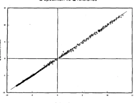
The basis for selection of a given thermal conductivity as representative of the tested material is matching the interface heat fluxes. If a perfect match took place at each point of the calculations, a plot of heat flux calculated for the reference material, Q.. against that for the test specimen, Q., would form a line with slope one. But as the value of heat flux depends on the boundary conditions, relation of Q, to Q. may vary within the range of temperatures occurring during the test period.

Comparison of heat flux values (Q, and Q,) is used for the optimization of the HFC calculations (see Figure 3). This permits the use of four different criteria for analysis of uncertainty, namely:

Q

specimen vs

reference

"r---r---.,

,.

-i

1

.,

.,.

"

FIGURE 3. An example of cakulations where the plot of the specimen heal flux (y-axis) is shown againsllhe reference heat flux (x-axis) for optimum values of thermal conductivity and heat capacity.

170 M. T.BOMBERG ET Al.

Error and Flux vs Time

.. r-r---_._---_-r---,---,

..

-..

..

e

..

...

_.,

...

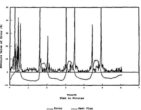
FIGURE 4. An example of coincidence between the standard error calculations for the ratio (Q, - Q,)/Q, and the reference heat flux in these calculations.

1. Slope of the regression line 2. Correlation coefficient

3. Curvature or non-zero intercept of the regression line 4. Polarity error

The absolute values of heat fluxes are chosen instead of the relative difference in these two heat fluxes, for instance (Qr - Q,)/Qr. The latter measure would depend on the value of the reference flux and cause excessive errors when the heat flux approaches zero. To illustrate the effect of heat flux reversals which are caused by solar radiation during a cold and sunny day, Figure 4 shows the standard error of the ratio of (Qr - Q,)/Qr.

Slope of the Regression Line

The slope of the regression line should equal one. If the reference heat flux is plotted on the"x"axis and the specimen heat flux is plotted on the "y" axis, slope greater than one indicates that the specimen heat flux is greater than

A Test Method to Determine Thermal Resistance under Field Conditions 17 1

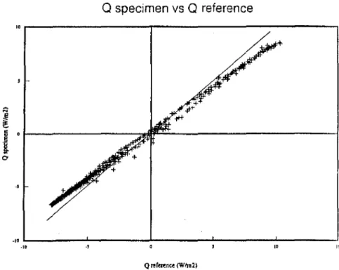
the reference heat flux at the interface boundary. Typicallyit indicatesthat the thermal conductivity coefficient assumed for the tested specimen is too high. Figure 5 illustrates such a case.

Correlation Coefficient of Linear Regression

The correlation coefficient is a measure of the scatter between data points in thermal properties estimated for each time step. A correlation coefficient dose to one indicates a small scatter or a good consistency of experimental points. A large scatter, i.e., lower correlation coefficient, may be caused by a phase shift in a heat flux measured under transient conditions, an effectlikely attributable to wrongly assumed heat capacity of the material (see Figure 6). A large scatter can also be caused by a large random variation of heat flux es-tablished on the reference material, an effect likely attributed to the error in the temperature measurements.

Curvature or Non-Zero Intercept of the Regression Line

These two kinds of deviations from a straight line passing through the

Q specimen vs Q reference 1 0 , . . - - ..,... - , 10

.,

.,.

l

l

.,

FIGURE 5. An example of the specimen heat flux plotted against that of the referencehell

flux when a 15 percent change in the intercept value of thermal conductivity was introduced(p

172 M. T.BOMBERG ET AL. Q specimen vs Q reference

"r---.,..---,

"

•

-,

FIGURE 6. An example of the specimen heat flux plotted against that of the reference heat flux when a 25 percent change in the heat capacity was introduced to the calculations shown in Figure3.

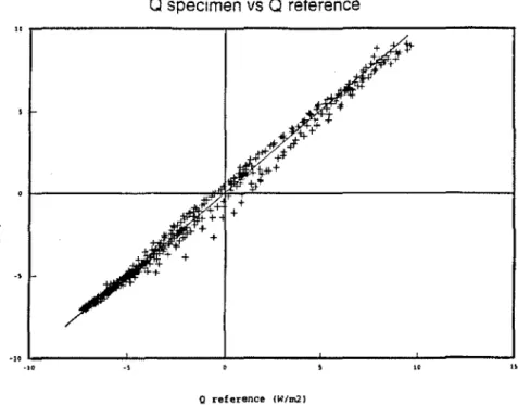
origin of the coordinate system may be observed on graphic representation ofdata (note that graphics are included in the HFC code). Figure 7 illustrates a deviation in the heat flux calculations performed on the same experimental data as those shown in Figure 3 caused by an error in the temperature coeffi-cient.

Polarity Error

There may be a systematic error in the heat flux calculated for the test specimen that is not shown by the correlation coefficient. To indicate the presence of such errors, a value of either - 1 or 1 is given each time the spec-imen heat flux is lower or higher than the reference value. The sum of these values divided by the number of calculations will indicate the significance of any systematic shift. A value near zero represents an equal balance of speci-men data points above and below the reference values.

SENSITIVITY ANALYSIS

parame-A Test Method to Determine Thermal Resistance umJer Field Conditions 173 QspecimenVB Q reference I! , . . . . - - - - ..,- ...,

"

.,

.,.

i

"

...

..

.,

FIGURE7. An example of the specimen heat flux plotted against that of the reference he:lt

flux when a 20 percent change in the temperature coefficient was introduced to the calculatio!l\ shown in Figure 3.

ters (intercept and temperature coefficient in thermal conductivity and con-stant specific heat), it was necessary to perform several series of calculations to assess the reliability of this calculational model. These calculations art'

described below. .

Sensitivity to a Change in Material Properties

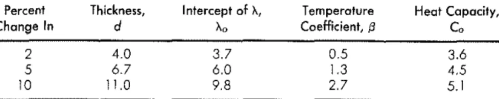
The sensitivity analysis was performed exclusively for low density ther-mal insulating materials. This analysis was performed with a sinusoidal data set generated to determine how the specific changes in material properties, time step or distance between two adjacent grid points would affect an error of the HFC calculations based on the same time step (e.g., 10 minutes). This analysis was compared with results obtained by Stephenson [5] and pro-vided valuable information about response to specific changes in the input data (see Table 1).

Changing the thickness of the specimen has the most significant effect on the standard error. Overestimating the specimen thickness caused the speci-· men heat flux to fall below the reference heat flux. Conversely, ｾｮ｣ｲ･｡ｳｪｮｧ

174 M. T. BOMBERG ET AL.

the value ofthermal conductivity increased the heat flux across the specimen with a magnitude of error similar to that caused by changing the specimen thickness,

Change in heat capacity (either caused by the change in specimen density or in the specific heat) caused a phase shift in relation to the theoretical curve (thermal lag) and slightly less significant error, Further adjustment of the heat capacity (from 2 percent to 10 percent) has only a slight effect on the standard error (the error increased from 3,6 percent to 5,1 percent). The specific heat of material may therefore be considered temperature indepen-dent in the range normally occurring under field conditions,

Finally, the change in temperature coefficient of thermal conductivity has the least effect on the standard error. It requires at least a 15 percent change to noticeably affect the flux calculations, and the significant effect on heat flux was observed only at high temperature peaks of the sinusoidal

tempera-ture variation.

Effects of simultaneous change in different material properties was also

examined, The cumulative error was approximately 5.5 percent for 2 percent positive error in all properties and double that for 5 percent of error in all properties [4,5],

This analysis indicates that material properties such as thickness and

den-sity must be accurately measured for both reference and tested specimens.

Thermal conductivity at the standard test conditions (room temperature)

must also be carefully measured for each reference specimen. Determination

of the temperature coefficient of thermal conductivity for each reference

specimen appears less important.

Sensitivity to a Change in Calculation Parameters

Increasing the number of grid points for each material layer and reducing the duration of time steps at which the temperature meaSUrements are taken

Table 1. Percentage oferrorofheat fluxin the specimen(0.) ascalculated by

HFC fora sinusoidol change of surface temperature and compared with the

reference value when thickness (d), interceptofthermal conductivity (Ao),

temperaturecoefficient ofthermal conductivity ({3), and heat capacity (Co) are

each changed by the percentage shown [4],

Percent Thickness, Intercept ofh, Temperature Heat Capacity, Change In d Ao Coefficient,{3 _Co

2 4.0 3.7 0.5 3,6

5 6.7 6,0 1.3 4,5

A 'lest Method to Determine Thermal Resistance under Field Conditions 175

may increase the accuracy of the calculations, but at the cost of computation time. To optimize the conditions of HFC application, the calculations were performed with time steps of 1, 10 and 60 minutes and grid divisions of 10, 15 and 20 points.

It was observed that input of temperatures expressed as one minute aver-age exhibited a visible level of noise (oscillations around the averaver-age values). Conversely, data collected at 60 minute intervals appeared to miss a certain frequency of outdoor temperature changes. Yet, data collected every two

minutes, averaged over ten minutes and ascribed to the mean value of time,

provided a smooth and reliable representation of the outdoor climate

varia-tions.

Due to the nature of numerical calculations (Taylor's series expansion), as

stated earlier, a certain number of time steps must be calculated before the results can be considered sufficiently accurate. This also applies to

interrup-tions in continuity of the records. for instance, when eliminating

experimen-tal data with a large random error. Analysis of a sample of calculations per-formed on a 10 point grid showed convergence to the required level of

precision after five time steps.

Propagation of the Measurement Errors

Equation (5) shows that the heat flux is calculated from two

compo-nents - a steady state component (temperature gradient at the current time step) and a transient component (temperature gradient at two previous time

steps). The total uncertainty of the heat flux will be a combination of the uncertainty of both components: transient and steady state.

Muzychka [7], assuming that temperature variations between time steps are small because of the short time step used in these calculations (10 minutes) and that uncertainty inｾＭｦｵｮ｣ｴｩｯｮ is the same for each point of the material, showed that the relative uncertainty of Equation (5) will be in the vicinity of the steady state component,

I1q/q

=

+

+

where e'l and eA are the uncertainties in the 'lJ-function (integral of thermal

conductivity) and the slab thickness, respectively. Further analysis showed that, for a given time step and number of grid points, the intercept of ther-mal conductivity,Ao, and the ratio of heat capacity to thermal conductivity have higher significance than other factors affecting the uncertainty of results.

An overall uncertainty in the thermal conductivity coefficient determined during the analyzed application of the test method has been foundtobe be-tween 4 and 7 percent [7]. Approximately 3.5 percent was attributed to

176 M. T. BOMBERG ET Al.

thickness and density determination and thermal properties of the referenct material, and 0.5 to 3.5 percent was attributed to uncertainty in thermal properties of the tested material.

APPLICATION OF THE HFC CODE TO FIELD MEASUREMENTS A roof exposure box which houses 600 X 600 mm square test specimens is shown in Figure 8 [11]. A reference material (glass fiber board with aver-age density of 112 kg/mJ _{and 24.4 mm thickness) was placed on a 12 mm}

thick plywood substrate. As shown in Figure 1, nine uniformly distributed thermocouples were used to measure each of its surface temperatures. A 50 mm thick test specimen was then placed on top of the reference specimen and six thermocouples were placed on its top surface. Edge insulation was placed to fix the test specimen position in the frame of exposure box and the 12 mm thick fiberboard overlay was placed on its top. A black EPDM (eth-ylene prop(eth-ylene diene monomer) membrane was used to cover the test assembly. The EPDM membrane was loosely laid and held in place by clips around the box's perimeter.

The surface temperatures were recorded at two-minute intervals and aver-aged for each ten minute period by an automated data acquisition system [7]. Field measurements were started at the beginning of February; however,

Fiberboard OM

Test Space

=

canst

=

=

=

=

=

=

---FIGURE 8. A roofing exposure box as used for measuring the thermal resistance of different polymeric foams manufactured with non-CFC blowing agents [11].

A nst Method to Determine Thermal Resistance under Field Conditions 177

large temperature variations inside the exposure box coupled with daily and periodic temperature variations that occurred during the early spring made. the calculations imprecise. Kossecka et al. [12], discussing the effect of ther-mal mass distribution within the wall on a transient heat flux that would be measured on a wall surface, showed that the heat flux is generally more sen- , sitive to the temperature difference in the vicinity of the analyzed surface than in the vicinity of the opposite surface. As HFC analysis is solely based

on temperatures measured on each surface of the reference material, the

analysis [12] implies the need to reduce the "noise" temperature fluctuations

on the inner surface of the reference material.

Indeed, when the temperature control within the exposure box was im-proved (namely, the electric baseboard heater was replaced with a large ca-pacity heating/cooling bath and heat exchanger and a continuously operating fan), the precision of HFC calculations was significantly im-proved. Therefore, only the results obtained after the change of the heating system are reported in this paper.

A special test series was performed to evaluate the reproducibility of the

method and to examine if moisture movement within the reference material

affects the measured field performance of the test material. This test series involved two identical specimens of expanded (XPS) and extrudcd polystyrene (EPS) tested in contact with the Same reference material (glass fiber insulation); each of them was provided with different boundary

condi-tions for moisture transport. One of these reference specimens was open to

the air and the other was sealed in a polyethylene bag. Thus, this test series comprised four tests.

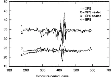
Figure 9 shows the thermal resistance of EPS and XPS foams determined with the HFC computer code and recalculated to mean temperature of 24°C, i.e., the temperature used in standard laboratory testing. Figure 9 shows a high repeatability of thermal resistance determined with different

reference specimens; in addition, it shows that the difference between tests

performed with sealed and open GFI specimens is small.

Furthermore, R-values of the EPS foam measured under laboratory con-ditions were practically identical to those measured under field concon-ditions. Thermal resistivity of 23.7 (m K)/W was determined under field conditions, while eight laboratory tests gave a mean value of 23.95 (m K)/W with a standard deviation of 0.32 (m K)/W [11]. This figure also shows that thermal resistance was determined with high precision during all the seasons except for the period of early spring (410 to 430 days in Figure 9). A probable cause for the anomaly shown in Figure 9 is discussed below.

EPS is an air filled foam and is therefore expected to have an invariable thermal resistance throughout the whole year. XPS foam has already reached the second stage of the aging process and is also expected to show

M, T. BOMBERG ET AL. 700 600 1-XPS 2 - XPS sealed 3 - EPS sealed 4-EPS 500 400 300 200 178 50 45

s:

SZ

S

'en

...

Exposure period, days

FIGURE9. Thermal resistivity, (m K)/W, recalculated to 24°C versus exposure period, Com-parative measurements were performed on EPS and XPS using both the open and the sealed specimens of the reference material.

only a small change of thermal resistance during the year, Indeed, these foams behaved in the expected manner over the whole testing period except for a short period at the beginning of spring when an apparent thermal resistivity of the foams exhibited strong variations. While it is not known whether it was the test or the reference material that was affected by some additional effects, there may be a number of causes. The most probable causes for these variations are an increased fluctuation of temperature inside the exposure box, frequent reversal of heat flow occurring at this season, or movement of moisture within the test system.

All in situ tested foams and reference materials are sandwiched between two wood based materials (waferboard substrate and fiberboard overlay) which contain some moisture. In the presence of a thermal gradient, this moisture will move towards the cooler side. During sunny but cold days, when the temperature on the cold side fluctuates, causing significant reversal of heat flows, this moisture is pushed back and forth, introducing a change in transient thermal properties measured under field conditions.

This change, being related to condensation and the evaporation cycle of moisture, depends on a combination of two material properties-vapor permeability and hygroscopic moisture content of the material. Figure 9 in-dicates that even though a moisture movement has not affected the reference

ATest Method to Determine Thermal Resistance under Field Conditions 179

GFI materialto a significant degree for most of the test period, it may have some effect on thermal performance of the analyzed test system during early spring when the prevailing warm climate causes significant drying of the overlay boards.

DISCUSSION

There are a number of factors that affect performance of thermal in-sulating materials under field conditions which cannot be easily predicted or tested in the laboratory. It is difficult to predict how much the foam insula-tion is affected by daily and seasonal temperature variainsula-tions, particularly when these processes affect aging and weathering of the foam and may even result in some accumulation of moisture inside the foam. One may, there-fore, prefer to measure thermal resistance when the foam is exposed to field conditions. One such method is presented in this paper.

As previously mentioned, if the response period of the heat flow trans-ducer is much shorter than the period of the tested system and if the HFT was calibrated as a function of temperature, one may also use the HFT for

determination of thermal perfonnance under transient conditions. The pre-cision of these measurements is, however, significantly reduced when

tem-perature conditions at the material boundary change with the frequency comparable to the response factor of HFT. Furthermore, as thermal proper-ties ofinsulating materials vary with temperature, using steady state approx-imation leads to a non-linear equation system.

The method described here alleviates most of the above mentioned

short-comings and determines thermal resistance under transient conditions where

a tested material slab is placed in contact with the reference material slab and temperatures of all the slab surfaces are recorded. Both materials are treated as homogeneous and their thermal properties (thermal conductivity and specific heat) are assumed to be linear functions of temperature. Use of Kir-choff's potential function instead of thermal conductivity linearizes the equation system for the range of temperatures in which linear relation of thermal conductivity on temperature holds. The code calculates heat flux at

the interface and finds a match within sensitivity and truncation errorsof the numerical method. Even though thermal properties of the test specimen are initially guessed, the process of simultaneous optimization of a few hundred data points (one test series lasts over a period of a few days) results in the most probable set of material properties.

Finally, applying the HFC method to field measurements highlights the

importance of precise interior temperature control. An improvement of

tem-perature control within the exposure box resulted in increased precision of HFC measurements. This information, combined together with the results

CONCLUSIONS

of the sensitIvity analysis, permits successful application of the HFC method.

This paper presented the development and application of a test method to measure the thermal properties of a material under field conditions. Several conclusions may be drawn from this work:

1. The HFC algorithm for comparison ofheat flux on interface between the

reference and the test specimens was sufficiently accurate for the specified input conditions (10 or more grid points, a maximum titne increment of

10 minutes averaged from 5 readings and ascribed to the middle of the period).

2. The optimization process that involves the slope, intercept and

correla-tion coefficient of linear regression was proven effective for selecting the

most probable set of material properties of the test material. The slope of the regression line is a strong function of thermal conductivity (primarily of the intercept in the linear representation of thermal conductivity vs temperature) and a much weaker function of thermal capacity. The

cor-relation coefficient is a strong function of heat capacity (density or

spe-cif,c heat of the material) and a much weaker function of thermal

conduc-tivity. Curvature and non-zero intercept of the regression line are strong

functions of the temperature dependence of thermal conductivity and

moderate functions of thermal conductivity intercept or specific heat.

3. Uncertainty of the HFC model appears to be a strong function of the

steady state component and a weak functionof thetransient components

of the heat flux at the contact boundary.

4. This analysis indicates that material properties such as thickness and den-sity must be accurately measured for both reference and tested specimens. Thermal conductivity at the standard test conditions (room temperature)

must also be carefully measured for each reference specimen.

5. The overall uncertainty of the field measurements was estimated to vary between 4 and 7 percent, of which 3.5 percent was attributed to the

uncertainty in the properties of the reference specimens.

6. Experience with the HFC method highlights the importance of precise

temperature control in the test box. Large temperature fluctuation inside

the exposure box gives rise to noisy heat flux calculations, reducing the precision of thermal property determination.

180 M. T. BOMBERG ET AL.

I

I

I

I

ACKNOWLEDGEMENTS

A 1est Method to Determine Thermal Resistance under Field Conditions 18J

were further developed in this project and who provided guidance, encour-agement and support. Many thanks go to John Lackey, who calibrated all reference specimens, to Roger Marchand, who developed interface and set the data acquisition system, and to Nicole Normandin, who patiently col-lected on disks more than 2,000,000 temperature readings per year, some of which are used in this paper.

REFERENCES

1. Bamberg, M. and K.R. Salvasan. 1985. "Discussion of Heat Flow Meter Ap-paratus and Transfer Standards Used for Error Analysis;'ASTM STP 879, pp.

140-153.

2. Wilkes, K. E. 1989. "Model for Roof Thermal Performance," ORNUCON-274,

Oak Ridge.

3. Anderlind, G. 1992. "Multiple Regression Analysis ofin situ Thermal

Measure-ments - Study of an Attic Insulated with 800 mm Loose Fill Insulation,"].

Ther-mal [nsul. and Bldg. Envs., 16:81-104.

4. Courville, G. E. and]. V. Beck. 1987. "Techniques for in situ Determination of Thermal Resistance of Light Weight Board Insulation;'Heat 1ranifer in Buildings

and Structures,Kuehn and Hickox, eds., ASME HTD, 78:7-15.

5. Stephenson. D. G. 1992. "The Calculation ofHeat Flux into a Slab

ofHomoge-neous Material That Has Thermal Conductivity and Volumetric Heat Capacity That Are Functionsof Temperature;' ]. of Thermal Insulation, 15:311-317.

6. Stevens, G. 1993. "Development of a Comparative Method to Estimate Thermal Resistanceof Homogeneous Insulation Materials under Field Conditions;' B.Se.

Thesis, U. of Western Ontario, Faculty of Engineering Science.

7. Muzychka,Y. S. 1992. "A Method to Estimate Thermal Resistance under Field Conditions;' National Research Council, Inst. for Research in Construction,

IRC Report 638.

8. Cacamburas, M. 1993. "HFC a Package to Calculate Heat Resistance under

Field Conditions," SP! Canada Report.

9. Pantakar, S. 1980. "Numerical Heat 1hnsfer and Fluid Flow," Hemisphere Pub!. Co.

10. Lai, M. "TURCOM: A Computer Code for Calculation of Transient,

Multi-Dimensional, Thrbulent, Multi-Component Chemically Active Fluid Flows;'

NRC Technical Report No. 27632.

1I. Bomberg, M. T. and M. K. Kumaran. 1994. "Laboratory and Roofing

Expo-sures of Cellular Plastic Insulation to Verify a Model of Aging;'Roofing Research

and Standards Development, ASTM STP1224,T.

J.

J.

eds" Philadelphia, PA: ASTM,

12. Kossecka, E.,

J.

J.