Publisher’s version / Version de l'éditeur:
Vous avez des questions? Nous pouvons vous aider. Pour communiquer directement avec un auteur, consultez
la première page de la revue dans laquelle son article a été publié afin de trouver ses coordonnées. Si vous n’arrivez pas à les repérer, communiquez avec nous à [email protected].
Questions? Contact the NRC Publications Archive team at
[email protected]. If you wish to email the authors directly, please see the first page of the publication for their contact information.
https://publications-cnrc.canada.ca/fra/droits
L’accès à ce site Web et l’utilisation de son contenu sont assujettis aux conditions présentées dans le site LISEZ CES CONDITIONS ATTENTIVEMENT AVANT D’UTILISER CE SITE WEB.
ACE '05: Proceedings of the 2005 ACM SIGCHI International Conference on
Advances in Computer Entertainment Technology, pp. 19-26, 2005
READ THESE TERMS AND CONDITIONS CAREFULLY BEFORE USING THIS WEBSITE. https://nrc-publications.canada.ca/eng/copyright
NRC Publications Archive Record / Notice des Archives des publications du CNRC :
https://nrc-publications.canada.ca/eng/view/object/?id=b97e570f-12fc-4483-a9c7-f612550ca465
https://publications-cnrc.canada.ca/fra/voir/objet/?id=b97e570f-12fc-4483-a9c7-f612550ca465
NRC Publications Archive
Archives des publications du CNRC
This publication could be one of several versions: author’s original, accepted manuscript or the publisher’s version. / La version de cette publication peut être l’une des suivantes : la version prépublication de l’auteur, la version acceptée du manuscrit ou la version de l’éditeur.
For the publisher’s version, please access the DOI link below./ Pour consulter la version de l’éditeur, utilisez le lien DOI ci-dessous.
https://doi.org/10.1145/1178477.1178480
Access and use of this website and the material on it are subject to the Terms and Conditions set forth at
Natural interaction with virtual objects using vision-based six DOF
sphere tracking
National Research Council Canada Institute for Information Technology Conseil national de recherches Canada Institut de technologie de l'information
Natural Interaction with Virtual Objects
Using Vision-Based Six DOF Sphere
Tracking*
Bradley, D., and Roth, G.
June 2005
* published in Advances in Computer Entertainment Technology. June
2005. NRC 48212.
Copyright 2005 by
National Research Council of Canada
Permission is granted to quote short excerpts and to reproduce figures and tables from this report, provided that the source of such material is fully acknowledged.
Natural Interaction with Virtual Objects Using
Vision-Based Six DOF Sphere Tracking
Derek Bradley
School of Computer Science Carleton University
Ottawa, Canada
[email protected]
Gerhard Roth
Institute for Information Technology National Research Council of Canada
Ottawa, Canada
[email protected]
ABSTRACT
A common task in computer entertainment is the ability to interact with virtual 3D objects. Interacting with these objects using standard computer input devices such as a mouse and keyboard can often be a difficult task. For this reason, Tangible User Interfaces (TUIs) were developed to allow more natural interaction with complex virtual objects by manipulating physical objects in a familiar way. Ap-plying the movements of a physical object to control the movement of a virtual object is often done by embedding devices in the physical object, or by passively tracking the object. We present a new TUI system that includes a pas-sive optical tracking method to determine the six degree-of-freedom (DOF) pose of a sphere in a real-time video stream, and then apply the pose to a virtual object. Our tracking system is based on standard computer vision techniques and applications of 3D geometry. The pose of the sphere is accu-rately resolved under partial occlusions, allowing the object to be manipulated by hand without a tracking failure. We demonstrate the use of our TUI system to control virtual 3D objects in an interactive way, proving to be a useful tool for computer entertainment applications.
1.
INTRODUCTION
Natural interaction methods that consist of manipulating real physical objects to control virtual entities are often called Tangible User Interfaces (TUIs) [9, 4, 14]. For more than thirty years, people have relied primarily on screen-based text and graphics, combined with keyboards, mice and other electronic devices to interact with computers. The concept of manipulating more natural physical objects in the form of TUIs to control computer data is an emerging field. TUIs are important in computer entertainment as they pro-vide a simple and natural way to interact with many appli-cations such as real-time video games. TUI systems have been developed using wired inertial tracking, electromag-netic tracking, and wireless optical tracking systems.
We present a passive optical TUI system that operates by resolving the full six degrees-of-freedom (DOF) pose of a sphere from real-time video input. The six DOF pose is comprised of the three DOF location and the three DOF orientation of the sphere in the scene. We use a specially marked ball as the sphere, and we compute the pose us-ing standard computer vision techniques and applications of 3D geometry. Our method correctly determines the pose of the sphere even when it is partially occluded, allowing the sphere to be manipulated by hand without a tracking failure. We show how our technique can be used as a TUI to control 3D objects in a virtual environment using natural hand movements.
The remainder of this paper is organized as follows. Related TUI systems and other sphere tracking techniques are out-lined in Section 2. Our method to track a sphere in a real-time video stream is described in Section 3. Section 4 shows the results and analysis of our tracking method. Example entertainment applications that make use of our technique as a TUI are described in Section 5. Finally, we conclude with a discussion in Section 6.
2.
RELATED WORK
Three-dimensional input devices were first considered in the late 1970s by Aish [1] and Frazer et al. [6]. These systems use building blocks with embedded computation to deter-mine the geometry of a tangible model, built from rigidly connected blocks of known size and shape. Tangible user interfaces have since evolved to include passive tracking, in order to offer wireless 3D interaction without the require-ment of embedded devices in the physical object. Most sim-ilar to our approach, Fjeld and Voegtli [4] and Huang et al. [9] develop a TUI that uses a passive optical tracking method to determine the pose of the tangible object. Spe-cial markers are placed on a physical cube and a camera is used to track the cube in real-time. One disadvantage of the system is that the tracking accuracy of the cube markers is dependent on the angle between the marker-plane normal vector and the camera. So as the cube is manipulated, track-ing is not consistent. Also, the cube markers are prone to tracking error during occlusions. Our TUI method is based on sphere tracking to obtain a consistent computation of the pose from any orientation, even in the presence of occlusions. Sphere tracking consists of locating the perspective projec-tion of the sphere on the image plane and then determining the 3D position and orientation of the sphere from the
pro-jection. Since the projection of a sphere onto a plane is a circle, the problem of locating circles in images is of interest. The concept of finding circular objects and curves in images has been studied for many years. In general, there are two different types of algorithms for curve detection (typically circles and ellipses) in images, those that are based on the Hough transform [3, 15, 16], and those that aren’t [2, 10, 11, 12, 13]. It should be noted that this is not an exhaus-tive list of circle detection methods, since the main focus of this paper is not the circle detection technique. For sim-plicity, we use a fast color-based detection method that is less accurate than some previous methods, however our sys-tem is not dependent on this technique so more accurate methods could be applied. The problem of actual sphere tracking has been less studied in previous work. The first research on sphere detection in images was performed by Shiu and Ahmad [13]. In their work, the authors were able to find the 3D position (three DOF) of a spherical model in the scene. Safaee-Rad et al. [12] also provided a solution to the problem of 3D position estimation of spherical features in images. Most recently, Greenspan and Fraser [7] devel-oped a method to obtain the five DOF pose of two spheres connected by a fixed-distance rod, called a dipole. Their method resolves the 3D position of the spheres in the form of 3 translations, and partial orientation in the form of 2 rotations in real-time.
Our method is based on tracking colored dots on a non-planar surface. A similar approach was taken by Guenter et al. in an application to capture 3D geometry of facial expressions [8]. In their work, 182 fluorescent circular fidu-cials of different colors are manually glued to an actor’s face to provide sampling points in a recorded video image. The method to track the colored circles in an input image is similar to ours, however Guenter et al. make use of six cam-eras to recover the 3D geometry and position of the face, where our system makes use of the geometric symmetry of a sphere and can recover the 3D position and orientation using a single camera. As well, our system resides in a different application domain.
To our knowledge, our method is the first optical method to resolve the full six DOF pose of a sphere in a scene, using a single camera in real-time. Since our technique is also capable of handling partial occlusions, it can be used as a TUI to control the position and orientation of 3D objects in a virtual environment or computer entertainment application.
3.
SPHERE TRACKING
Our method to track a sphere consists of a number of stan-dard computer vision techniques, followed by several ap-plications of mathematics and 3D geometry. Tracking the sphere is divided into two phases, computing the sphere lo-cation and computing the sphere orientation.
3.1
Pre-Processing
The sphere used for tracking is a simple blue ball. In or-der to determine the orientation of the sphere, special dots were added to its surface for detection. The dots are made from circular green and red stickers, distributed over the surface at random. Sixteen green, and sixteen red point lo-cations were generated in polar co-ordinates, such that no two points were closer (along the sphere surface) than twice
the diameter of the stickers used for the dots. This restric-tion prevents two dots from falsely merging into one dot in the projection of the sphere on the image plane. To deter-mine the arc distance between two dots, first the angle, θ, between the two locations and the center of the sphere was computed as
θ = cos−1(sin(lat
1) · sin(lat2) +
cos(lat1) · cos(lat2) · cos(|lon1− lon2|)), (1)
where (lat1, lon1) is the first dot location, and (lat2, lon2) is
the second dot location in polar co-ordinates, and then the arc length, α, was calculated as
α = θ · M, (2) where M is the number of millimeters per degree along the circumference of the sphere (which is also the radius of the sphere). A valid point location is one where α is larger than twice the sticker diameter (26 millimeters to be exact) when compared to each of the other points.
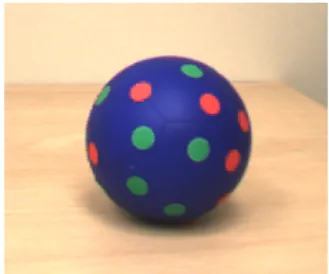
Once the thirty-two latitude and longitude locations were generated, the next step was to measure out the locations of the dots on the physical ball and place the stickers accord-ingly. Figure 1 shows the ball with the stickers applied to the random dot locations.
Figure 1: Sphere to be tracked in the video stream. In addition to the dot locations, the tracking process also requires knowledge of the angle between each unique pair of points (through the center of the sphere). Equation 1 was used to compute the angle for each of the 496 pairs, and the angles were stored in a sorted list.
3.2
Computing Location
Locating the sphere in a frame from a real-time video stream is a two step process. First, the perspective sphere tion is located on the image plane. Then, from the projec-tion in pixel co-ordinates, the 3D locaprojec-tion of the sphere in world co-ordinates is computed using the intrinsic parame-ters of the camera.
The projection of a sphere onto a 2D plane is always a circle. Since the ball was chosen to be a single color, the problem is to find a blue circle in the input image. To solve this problem we convert the input image from the Red-Green-Blue (RGB) color space to the Hue-Saturation-Value (HSV) color space [5]. The use of HSV space allows sphere tracking under varying illumination conditions. The image, I, is then binarized using the pre-computed hue value of the blue ball
as a target value. The binary image is computed as follows; Bi= 8 < : 0 if Ii< (T − ǫ) 0 if Ii> (T + ǫ) 1 otherwise, (3) where T is the target hue, and ǫ is a small value to generate an acceptable hue window. In the special case that T −ǫ < 0, the computation for the binary image takes into account the fact that hue values form a circle that wraps around at zero. From the binary image, the set of all contours are computed. Since there are many contours found, the next step is to filter out the ones that are not likely to be a projection of a sphere. The process searches for the contour that most closely approximates a circle; so all contours are tested for size and number of vertices. Testing the size of the contours, computed as the pixel area Ai occupied by
contour i, removes unwanted noise in the image. A contour must occupy 1500 pixels in order to be processed further. It is then assumed that any circle will contain a minimum number of vertices, in this case eight. For each contour that passes the above tests, the minimum enclosing circle with radius riis found, and then the following ratio is computed;
Ri=
Ai
ri
. (4)
For a circle, this ratio is a maximum. Therefore the con-tour that maximizes Ri is chosen as the projection of the
sphere on the image plane, since that contour most closely represents a circle. Figure 2 illustrates these steps to find the projection.
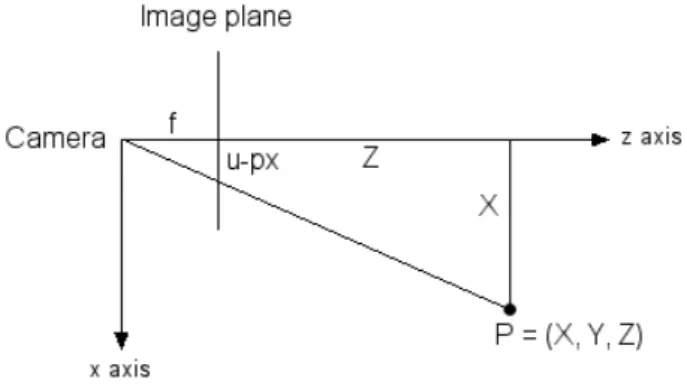
If the perspective projection of the sphere was found in the input image, processing continues to the second step in lo-cating the sphere, which is to calculate its 3D location in world co-ordinates. The scene is a 3D co-ordinate system with the camera at the origin. Assuming that the intrinsic parameters of the camera are known in advance, namely the focal length and principal point, the location of the sphere can be computed from its perspective projection. Consider the top-down view of the scene in Figure 3, showing the per-spective projection of a single 3D point. The focal length of the camera is f and the principal point is (px, py). If the
Figure 3: Perspective projection of a 3D point. perspective projection of the point P = (X, Y, Z) in space lies at pixel (u, v) on the image plane then
u − px f = X Z (5) X = Z · (u − px) f , (6) and similarly Y =Z · (v − py) f . (7)
So we have X and Y expressed in terms of the single un-known value Z. For the case of the sphere, the point P can be taken as the sphere center in world coordinates, and then the problem is to find the value of Z for this point. This is solved based on weak perspective projection, which assumes that the sphere will always be far from the image plane [7]. Consider a point Pj on the surface of the sphere
which maps to a pixel on the circumference of the sphere projection. The weak perspective projection assumption en-sures that the line connecting Pj with P is parallel to the
image plane. Figure 4 illustrates the scenario, where the sphere of radius R projects to the circle of radius r. Now by
Figure 4: Computing the Z value for a sphere using weak perspective projection.
similar triangles,
Z = R · f
r . (8)
Equation 8 is now used in conjunction with Equation 6 and Equation 7 to find the 3D location of the sphere in the scene, given the current center, (u, v), and the radius, r, of the perspective projection.
3.3
Computing Orientation
The red and green dots on the surface of the sphere are used to compute its three DOF orientation. The process to compute the orientation is outlined as follows:
1. Locate the projections of the red and green dots on the image plane.
2. Compute the polar coordinates of the dots, assuming that the center of projection is the north pole. 3. Choose the two dots that are closest to the center
of projection and compute the angle between them (through the center of the sphere).
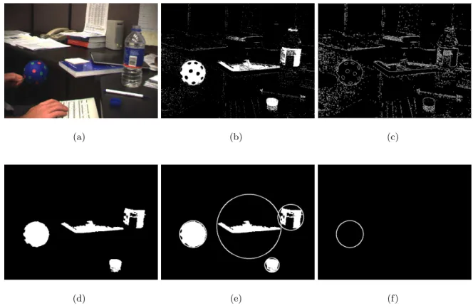
(a) (b) (c)
(d) (e) (f)
Figure 2: Locating the perspective sphere projection. a) Input image; b) Binary image; c) Set of all contours; d) Filtered contours; e) Minimum enclosing circles; f ) Most circular contour (chosen to be the projection of the sphere).
4. Use the sorted list of pairs to find a set of candidate matches to the two chosen dots.
5. For each potential match, orient the virtual sphere to align the two chosen dots and compute a score based on how well all the dots align.
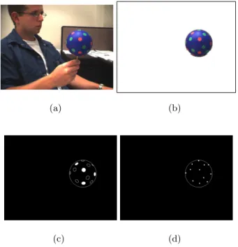
The projections of the green and red dots are located using hue segmentation to binarize the input image, similar to locating the projection of the sphere. Since we have already computed the projection of the sphere, we can restrict the search space to only the part of the input image that is inside the projection. In this case, the contours retrieved are expected to be ellipses. Therefore, an ellipse is fit to each contour that is found and its center location in screen coordinates is computed. Figure 5 illustrates the process of locating the dots on the sphere surface.
Once the dots are located, the center of the sphere projec-tion is considered to be the north pole of the sphere, with a latitude value of −π/2 radians and longitude value of zero. Then the relative polar coordinates of the projected dots are computed. Let the center of the sphere projection on the image plane be (uc, vc), the projection of dot i be (ui, vi),
and the point on the circumference of the sphere projec-tion directly below (uc, vc) be (ub, vb). Figure 6 illustrates
the situation. Notice that uc = ub. The distance, A,
be-tween (ui, vi) and (uc, vc), and the distance, B, between
(ui, vi) and (ub, vb) are computed easily. The distance
be-tween (uc, vc) and (ub, vb) is the radius of the circle, r. Since
we assume the projection is a top down view of the sphere with the north pole at the center of the circle, the relative longitude, loni, of dot i is the angle b, which can be
com-puted by a direct application of the cosine rule; loni= b = cos−1(
A2+ r2− B2
2 · A · r ). (9) Note that if ui< uc, then loni is negative. The calculation
for the relative latitude, lati, is then
lati= −cos−1(
A
r). (10)
Each dot that was found in the input image now contains polar coordinates relative to an imaginary north pole at the center of the projection. The assumption of the north pole location and the computation of the relative polar coordi-nates was necessary in order to compute the arc length be-tween point locations from the projection of the surface dots. The next step is to choose the two dots that are closest to the center of the sphere projection and compute the angle, θ, between them using Equation 1. These dots are chosen be-cause they will contain the lowest error in polar coordinate location, since small variations in pixel location will result in only small variations in the polar coordinate computation. This angle θ is then used to find a set of possible matches for the two chosen dots from the pre-computed sorted list of all
(a) (b)
(c) (d)
Figure 5: Locating the projections of the dots on the sphere. a) Input image; b) Restricted input; c) Ellipses found for the red (filled) and green (un-filled) dots; d) Exact dot locations.
Figure 6: Computing relative polar coordinates.
pairs of dots. The set of possible matches is the set of pairs, such that the angle between each pair is within a small con-stant value, ǫ, of θ, and also such that the dot colors match the two chosen dots. The need for two separate dot colors is evident here, since too many matches are generated if only a single color is used. Each candidate pair is then tested to see how well that pair supports the two chosen dots. The pair with the most support is chosen as the matching pair. The original set of dot locations in polar coordinates can be thought of as a virtual sphere in a standard orientation. The process to test a candidate pair is to rotate the virtual sphere in order to line up the two points of the pair with the two chosen points in the projection on the image plane. The rotation is accomplished in two steps. First, the virtual sphere is rotated about an axis perpendicular to the plane formed by the first point in the pair, the first chosen point and the center of the sphere. This rotation aligns the first point. Then, the virtual sphere is rotated about the vec-tor connecting the center of the sphere to the first point in
order to align the second point. Once the virtual sphere is aligned to the two chosen points, a score is computed for this possible orientation. The validity of a given orienta-tion is evaluated based on the number of visible dots in the perspective projection that align to real dots of the correct color on the virtual sphere, as well as how closely the dots align. Visible dots that do not align to real dots decrease the score, as do real dots that were not matched to visible dots. All points are compared using their polar coordinates, and scores are computed differently based on the latitude values of the points, since points that are closer to the center of the sphere projection should contain a smaller error than those that are farther from the center. This is the case because an error of one pixel in the input image results in a smaller error in latitude value near the center of the sphere projec-tion than near the edge. Two points, P 1 and C1, are said to match if the angle, θ, between them satisfies the following inequality;
θ < (1 + latC1·
2
π)(α − β) + β, (11) where α is a high angle threshold for points that are farthest from the center of projection, and β is a low angle thresh-old for points that are at the center of projection. In our experiments, values of α = 0.4 radians and β = 0.2 radians produce good results. Using Equation 11, the number of matched dots is calculated as Nm for a given orientation.
Let Nv be the number of visible dots that are not aligned
to real dots, let Nr be the number of real dots that are not
matched with visible dots (and yet should have been), and let θi be the angle between the matching pair. Then the
score, σ, is computed as follows; σ = PNm i=1ˆ(1 + lati·2π)(α − β) + β − θi˜ − PNv i=1ˆ(1 + lati·π2)(α − β) + β˜ − PNr i=1ˆα − (1 + lati·2π)(α − β)˜ . (12)
In the case that the two chosen dots are the same color, each pair is tested again, after switching the two positions. The orientation that yields the highest score is chosen as the matching orientation for the sphere in the scene.
4.
RESULTS AND ANALYSIS
Results of the sphere tracking method show efficient detec-tion of the sphere with six DOF from a real-time video stream. Figure 7 shows a screenshot of the sphere in an arbitrary orientation with the matching orientation of the virtual sphere shown in the upper left corner.
4.1
Usability
Our sphere tracking TUI system operates at an average frame-rate of 15 frames per second on a Pentium 4 processor at 3.4Ghz using a color Point Grey Dragonfly camera with a resolution of 640x480 pixels. This provides a fast interactive method that can be used in many computer entertainment applications. Although tracking errors do affect the usabil-ity of our method, a brief analysis of the errors can lead to a method for improving usability. As the video results demonstrate, most tracking errors occur in the orientation computation of the sphere, and they occur in a single frame where numerous previous and following frames provide suc-cessful tracking. By averaging the result of the sphere track-ing over a few successive frames, individual tracktrack-ing errors
Figure 7: Sphere with matched virtual orientation.
become negligible and the usability of our system is greatly improved.
4.2
Occlusion Handling
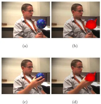
One of the main benefits of our sphere tracking method is that the tracking does not fail during partial occlusions. Oc-clusion is when an object cannot be completely seen by the camera. This normally results from another object com-ing in between that object and the camera, blockcom-ing the view. The sphere tracking method chooses the best-fit cir-cle of the correct hue in the projection of the scene as the location of the sphere. This means that objects can par-tially occlude the sphere and yet it may still be chosen as the best-approximated circle. Also, since the minimum en-closing circle is computed from the contour, only the pixels representing 180 degrees of the circumference plus one pixel are required in order to determine the location of the sphere with the correct radius. For this reason, up to half of the sphere projection may be occluded and yet its 3D location can still be computed correctly. Furthermore, the tracking process does not require that all of the dots on the surface of the sphere be visible in order to determine the orientation of the sphere. Since the matched orientation with the best score is chosen, it is possible to occlude a small number of the dots and yet still track the orientation correctly. The ability to correctly handle partial occlusions is very benefi-cial in a sphere tracking process because it allows a person to pick up the sphere and manipulate it with their hands. Figure 8 shows how the sphere tracking does not fail under partial occlusion. In this screenshot, the sphere is used in an augmented reality application where a teapot is being augmented at the location and orientation of the sphere in the scene.
4.3
Orientation Error
The accuracy of our TUI system will now be analyzed. Lo-cating the 3D position of a sphere in an image is not a new idea, however the novelty of this paper lies in the method to determine its 3D orientation. Therefore, we will study only the results of the orientation computation.
In order to compute an error on the 3D orientation compu-tation of our tracking method, the sphere must be manually placed in the scene with a known orientation. This is a very difficult task because the sphere is a physical object and it is nearly impossible to determine its actual orientation in
(a) (b)
(c) (d)
Figure 8: Handling partial occlusions. a) Non-occluded input; b) Non-Non-occluded tracking; c) Oc-cluded input; d) OcOc-cluded tracking.
the scene before performing the tracking. For this reason, a virtual 3D model of the sphere was built with exact pre-cision. Then the virtual sphere model was rendered on top of live video images at chosen orientations, and the track-ing procedure was applied. The actual orientation and the tracked orientation were then compared each frame to de-termine a tracking error. Specifically, 100000 video frames were captured with the virtual sphere inserted at random orientations. Since we assume weak perspective projection, the virtual sphere was constrained to X and Y values of zero, such that the perspective projection was always in the center of the image plane. The Z value of the sphere was chosen randomly to simulate different distances from the camera. The question that remains is how can one 3D ori-entation be compared to another? It was decided that a particular orientation of the sphere would be defined by the quaternion rotation that transformed the sphere from its standard orientation. A quaternion is a 3D rotation about a unit vector by a specific angle, defined by four parameters (three for the vector and one for the angle). The actual ori-entation of the inserted sphere and the result of the tracking method were compared by analyzing the two corresponding quaternion rotations. This produced two errors, one error on the quaternion axis and one in the angle. The axis error was computed as the distance between the end points of the two unit vectors which define the quaternions, measured in units of space. The angle error was simply the difference between the two scalar angle values. So for each of the 100000 chosen orientations we have a six-dimensional vector (four dimensions for the quaternion orientation and two for the errors) to describe the tracking error. Visualizing the error for analysis is a non-trivial task. Even if the errors are analyzed separately, it is still difficult to visualize two five-dimensional vectors. However, we realize that the
re-sults of the error analysis will indicate how well the tracking method is able to determine the best match to the perspec-tive projection of the dots on the surface of the sphere. This, in turn, will give some feedback on how well the dots were placed on the sphere and could indicate locations (in polar coordinates) where the dots were not placed well. So instead of visualizing all four dimensions of a quaternion, the polar coordinates of the center of the perspective projection were computed for each orientation. This assumes that a perspec-tive projection of the sphere under any 2D rotation will yield similar errors, which is a reasonable assumption. Now the errors can be analyzed separately as two three-dimensional vectors (two dimensions for the polar coordinates and one for the error). Figure 9 is a graph of the average error in the quaternion axis over all the polar coordinates, and Fig-ure 10 is a similar graph of the average error in quaternion angle. In both graphs, darker points indicate greater error and white points indicate virtually no error. It is clear to
Figure 9: Analysis of error on quaternion axis.
Figure 10: Analysis of error on quaternion angle. see from Figure 9 that the greatest error in quaternion axis is concentrated around the latitude value of −π/2 radians, that is to say, the north pole of the sphere. Figure 10 indi-cates that the error in quaternion angle is relatively uniform across the surface of the sphere. Additionally, the overall average error in quaternion axis for a unit sphere is 0.034 units, and in quaternion angle is 0.021 radians. This
analy-sis shows that the sphere tracking method presented in this paper has excellent accuracy.
5.
APPLICATIONS
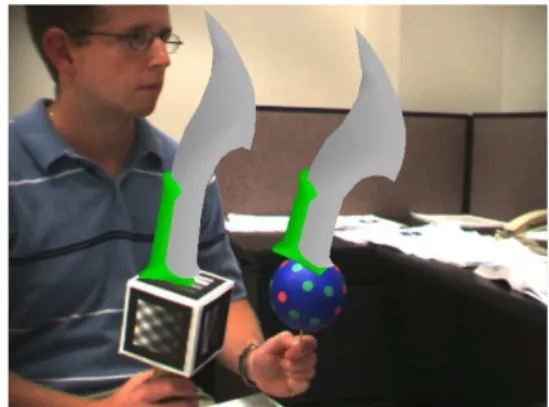
Resolving the six DOF pose of a sphere in a real-time video sequence can lead to many interactive computer entertain-ment applications. One application that was hinted at in the previous section is in the field of augmented reality. Aug-mented reality is the concept of adding virtual objects to the real world. In order to do this, the virtual objects must be properly aligned with the real world from the perspective of the camera. The aligning process typically requires the use of specific markers in the scene that can be tracked in the video, for instance, a 2d pattern on a rigid planar ob-ject. An alternate way to align the real world and the virtual objects is to use the marked sphere and tracking method de-scribed in this paper. Once the location and orientation of the sphere is calculated, a virtual object can be augmented into the scene with the same pose. The equivalent planar pattern method would be to use a marked cube [4, 9]. Fig-ure 11 shows an augmented reality application using both a marked cube and our sphere method to augment a virtual sword for an augmented reality video game. The main ad-vantage of tracking the sphere over tracking the cube is that the sphere is more robust under partial occlusions.
Figure 11: Augmented reality application of the sphere tracking method.
Another TUI application of our sphere tracking method is to use the sphere as an input device for an interactive 3D application. In many applications, users must interactively control 3D objects on a computer screen. Some systems re-quire a combination of key presses and mouse movements to rotate and translate the objects. This is often a complicated task that requires a learning period for the users. Our TUI sphere tracking method could be used to control a virtual object, if the pose of the sphere were mapped directly to the orientation of the object on the screen. Then the natu-ral handling and rotating of the device would translate into expected handling and rotating of the virtual object. In ad-dition, our system can be used to control the movement of an avatar or the user in a 3D game where six degree-of-freedom movement is possible.
6.
CONCLUSION AND DISCUSSION
We have presented a passive optical TUI method to provide interaction with computer data using natural manipulation of a physical object. Our system includes tracking the sixDOF position and orientation of a sphere from a real-time video stream. The sphere is a simple blue ball with 32 ran-domly placed green and red dots. Tracking consists of lo-cating the perspective projection of the sphere on the image plane using standard computer vision techniques, and then using the projections of the dots to determine the sphere orientation using 3D geometry.
Previous methods use a marked cube with planar patterns on its six sides. However, the tracking accuracy is inconsis-tent as the cube is manipulated because the accuracy de-pends on the angle between the pattern normal vector and the camera. Our sphere-based technique allows for more consistent tracking independent of the orientation. Another important advantage of our method is that partial occlu-sions are handled correctly, allowing the sphere to be picked up and manipulated by hand. This provides a more natural interaction method for controlling virtual objects than the cube-based technique.
Some drawbacks do exist with our tracking method, includ-ing multiple or overlappinclud-ing scene objects of the target color, and errors due to manually placing the dots on the ball. As well, two-handed interaction can cause tracking incon-sistencies due to the irregular occlusion of the sphere. This research has unveiled an interesting open problem; namely, how can N dots be placed on the surface of a unit sphere such that the perspective projection of the sphere in any ori-entation is maximally unique. Solving this problem would guarantee maximum performance for the TUI system de-scribed in this paper. Our sphere tracking fails when the projections of two different orientations appear too similar on the image plane. Placing the surface dots in a way which maximizes the uniqueness of any projection would optimize the method to resolve the 3D orientation of the sphere.
7.
ACKNOWLEDGEMENTS
This work was supported by the Natural Sciences and En-gineering Research Council of Canada.
8.
REFERENCES
[1] R. Aish. 3d input for caad systems. Computer-Aided Design, 11(2):66–70, Mar. 1979.
[2] T.-C. Chen and K.-L. Chung. An efficient randomized algorithm for detecting circles. Comput. Vis. Image Underst., 83(2):172–191, 2001.
[3] R. O. Duda and P. E. Hart. Use of the hough transformation to detect lines and curves in pictures. Commun. ACM, 15(1):11–15, 1972.
[4] M. Fjeld and B. M. Voegtli. Augmented chemistry: An interactive educational workbench. In IEEE and ACM International Symposium on Mixed and Augmented Reality (ISMAR 2002), pages 259–260, September 2002. Darmstadt, Germany.
[5] J. D. Foley, A. van Dam, S. K. Feiner, and J. F. Hughes. Computer graphics: principles and practice (2nd ed.). Addison-Wesley Longman Publishing Co., Inc., 1990.
[6] J. Frazer, J. Frazer, and P. Frazer. Intelligent physical three-dimensional modelling system. In Proceedings of
Computer Graphics 80, pages 359–370, 1980. Online Publications.
[7] M. Greenspan and I. Fraser. Tracking a sphere dipole. In 16th International Conference on Vision Interface, June 2003. Halifax, Canada.
[8] B. Guenter, C. Grimm, D. Wood, H. Malvar, and F. Pighin. Making faces. In SIGGRAPH ’98: Proceedings of the 25th annual conference on Computer graphics and interactive techniques, pages 55–66. ACM Press, 1998.
[9] C.-R. Huang, C.-S. Chen, and P.-C. Chung. Tangible photorealistic virtual museum. IEEE Computer Graphics and Applications, 25(1):15–17, 2005. [10] E. Kim, M. Haseyame, and H. Kitajima. A new fast
and robust circle extraction algorithm. In 15th International Conference on Vision Interface, May 2002. Calgary, Canada.
[11] G. Roth and M. D. Levine. Extracting geometric primitives. CVGIP: Image Underst., 58(1):1–22, 1993. [12] R. Safaee-Rad, I. Tchoukanov, K. C. Smith, and
B. Benhabib. Three-dimensional location estimation of circular features for machine vision. Transactions on Robotics and Automation, 8(5):624–640, 1992. [13] Y. Shiu and S. Ahmad. 3d location of circular and
spherical features by monocular model-based vision. In IEEE Intl. Conf. Systems, Man, and Cybernetics, pages 567–581, 1989.
[14] B. Ullmer and H. Ishii. Emerging frameworks for tangible user interfaces. IBM Systems Journal, 39(3-4):915–931, 2000.
[15] L. Xu, E. Oja, and P. Kultanen. A new curve
detection method: randomized hough transform (rht). Pattern Recogn. Lett., 11(5):331–338, 1990.
[16] H. K. Yuen, J. Illingworth, and J. Kittler. Detecting partially occluded ellipses using the hough transform. Image Vision Comput., 7(1):31–37, 1989.