Calibration of a microscopic traffic simulator

Calibration of a Microscopic Traffic Simulator

by

Mathew Kurian

Bachelor of Technology in Civil Engineering

Indian Institute of Technology, Madras, June 1997

Submitted to the Department of Civil and Environmental Engineering

in partial fulfillment of the requirements for the degree of

Rm

Master of

Science

in Transportation MASSAC HNELOINSTITUTE

at the

MASSACHUSETTS INSTITUTE OF TECHNOLOGY

FF140

February 2000

LIBRARIES

©

Massachusetts Institute of Technology 2000. All rights reserved.

Author ...

Department of 'ivil anA Environmental Engineering

November 1, 1999

Certified by.

...

Moshe E. Ben-Akiva

Edmund K. Turner Professor of Civil and Environmental Engineering

Thesis Supervisor

C ertified by ....

...-

...

-Mithilesh K. Jha

Research Associate, Center for Transportation Studies

Thesis Supervisor

C ertified by ....

...

Didier M. Burton

Research Associate, Center for Transportation Studies

Thesis Supervisor

Accepted by.

...-.-.-.

Daniele Veneziano

Chairman, Department Committee on Graduate Students

Calibration of a Microscopic Traffic Simulator

by

Mathew Kurian

Bachelor of Technology in Civil Engineering

Indian Institute of Technology, Madras, June 1997

Submitted to the Department of Civil and Environmental Engineering on November 1, 1999, in partial fulfillment of the

requirements for the degree of Master of Science in Transportation

Abstract

A systematic calibration study was performed on a microscopic traffic simulator-MITSIM. An optimization based framework was developed for calibration. Car-Following model parameters were identified for calibration and experimental design methodology was used to determine the set of sensitive parameters. Calibration was performed by minimizing the deviation between the simulated and observed values of speed. Two different objective function forms were formulated for quantifying the deviation between the simulated and observed values. The search space and the opti-mum parameter values for the two objective function forms were compared. The effect of stochasticity in calibrating the parameter values was also studied. Stochasticity was found to have a significant impact on the optimal parameter values. It was found that though calibration is an intricate process, the performance of the simulator can be substantially improved by an appropriate calibration study.

Thesis Supervisor: Moshe E. Ben-Akiva

Title: Edmund K. Turner Professor of Civil and Environmental Engineering

Thesis Supervisor: Mithilesh K. Jha

Title: Research Associate, Center for Transportation Studies

Thesis Supervisor: Didier M. Burton

Acknowledgements

I would like to thank my supervisors Prof. Moshe Ben-Akiva, Mithilesh Jha, and Didier Burton for their guidance and support at all stages of my research. I would also like to thank SAMTECH, for the evaluation version of Boss/Quattro. This software proved to be very useful for implementation and analysis.

I would also like to thank the Centre for Transportation Studies and the Central Artery/Tunnel project for providing funding for my research. I would also like to thank the Dept. of Civil Eng. for the opportunity to work as a Teaching Assistant for the course 1.00 for three semesters.

I would also like to thank Cynthia Stewart and her staff, and Leanne Russell for their support.

My special thanks are also due to Sydney Miller for her friendship, and all the folks at the CTS office, Janet, Nancy, and Mary, who made CTS so much more lively and enjoyable.

I also want to thank my officemates Bruno, Tomer, Masroor, Seong, Atul and Sreeram and also Vinay, Salal and Nadine. My special tons of thanks are due to my friends Debjit and Petros for making my stay at MIT so much more enjoyable.

I would like to thank Prof. Nigel Wilson for his support, guidance, understanding and his eagerness and willingness to help.

Finally I would like to thank my Dad, Mom and my sister Jinu for their under-standing and support.

Contents

1 Introduction

1.1 Literature Review . . . . 1.1.1 Traffic Simulation Models 1.1.2 Microscopic Simulator .

1.1.3 Calibration Studies . .

1.2 Calibration Framework . . . . 1.3 Thesis Objective . . . . 1.4 Thesis Outline . . . .

2 Simulator, Parameters and Data

2.1 MIcroscopic Traffic SIMulator-MITSIM . . . . 2.1.1 Main Simulation Models . . . . 2.2 Car-Following Model . . . . 2.2.1 Car-Following Parameters . . . . 2.3 Simulation Network and Data . . . . 2.4 C onclusion . . . .

3 Sensitivity Analysis

3.1 Responses ... ... ... ... . . . . .. . . . . 3.2 Experimental Design . . . . 3.2.1 2 k Factorial Design . . . .

3.2.2 Fractional Factorial Designs . . . . 3.2.3 Response Functions . . . . 10 11 11 11 11 14 15 16 17 17 19 19 20 22 24 28 29 29 30 32 33

3.2.4 Stochasticity . . . . 33

3.3 R esults . . . . 34

3.4 Conclusion. . . . . 37

4 Calibration 42 4.1 Response Selection . . . . 43

4.2 Objective Function Forms . . . . 43

4.3 Stochasticity . . . . 44

4.4 Optimization . . . .. 47

4.4.1 Optimization Methodology . . . . 48

4.5 R esults . . . . 48

4.5.1 Comparison of the Spread of the Objective Functions . . . . . 49

4.5.2 Results for a Fixed Random Number Seed . . . . 50

4.5.3 Sampling Distribution of Optimal Parameter Values . . . . 57

4.6 Conclusion . . . . 66

5 Summary, Conclusions and Research directions 69 5.1 Summary and Conclusion . . . . 69

5.2 Research Directions . . . . 70

A Boss/Quattro 72 A.1 Introduction . . . . 72

A .2 Structure . . . . 72

A.3 Using Boss/Quattro with MITSIM . . . . 75

A.3.1 Environment Setup . . . . 75

A.3.2 Studies . . . .. . . . 77

A.3.3 Sensitivity Study . . . . 78

A.3.4 Optimization study . . . . 80

A.4 Conclusion . . . - - - . - . . .. . . . . 80

B MITSIM-Parameters 82

List of Figures

2-1 1-880 Network . . . . 23

2-2 Comparison between simulated and field data. . . . . 25

2-3 Contour plots of simulated and field data. . . . . 26

2-4 Comparison of simulated and field data . . . . 27

3-1 Plot of the responses versus the design points . . . . 36

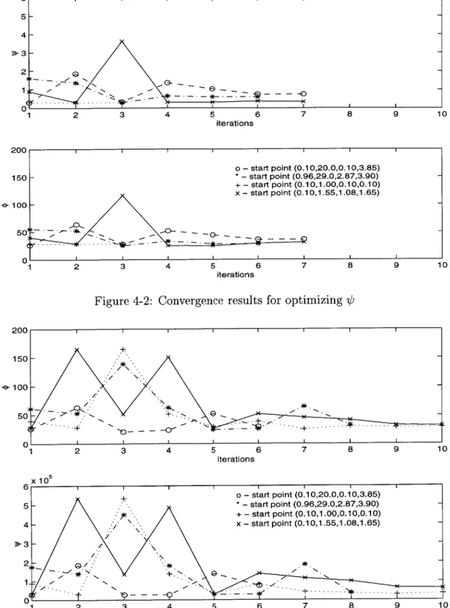
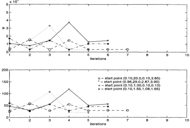
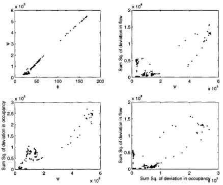
4-1 Illustrating the effect of stochasticity in calibrating parameter values . 46 4-2 Convergence results for optimizing 0 . . . . 51

4-3 Convergence results for optimizing

#

. . . . 51

4-4 Convergence results for optimizing 4 . . . . 52

4-5 Convergence results for optimizing

#

. . . . 52

4-6 Correlation plots . . . . 54

4-7 Comparison of simulated and observed data for parameter set 1 . . . 58

4-8 Comparison of simulated and observed data for parameter set 2 . . . 58

4-9 Comparison of simulated and observed data for parameter set 3 . . . 58

4-10 Comparison of simulated and observed data for parameter set 4 . . . 58

4-11 Contour plots for simulated and field data for parameter set 1 . . . . 59

4-12 Contour plots for simulated and field data for parameter set 2 . . . . 59

4-13 Contour plots for simulated and field data for parameter set 3 . . . . 60

4-14 Contour plots for simulated and field data for parameter set 4 . . . . 60

4-15 Comparison of simulated and field data for parameter set 1 . . . . 61

4-16 Comparison of simulated and field data for parameter set 2 . . . . 61

4-17 Comparison of simulated and field data for parameter set 3 . . . . 62

4-18 Comparison of simulated and field data for parameter set 4 . . . . 62 4-19 Comparison of simulated and observed data for parameter set obtained

by optim izing 0 . . . . 63 4-20 Comparison of simulated and observed data for parameter set obtained

by optim izing

4

. . . . 64 4-21 Contour plots for simulated and field data for parameter set 1 obtained

by optim izing 0 . . . . 64 4-22 Contour plots for simulated and field data for parameter set 2 obtained

by optim izing

4

. . . . 65 4-23 Comparison of simulated and field data for parameter set 1 obtained

by optim izing 4 . . . . 65 4-24 Comparison of simulated and field data for parameter set 2 obtained

by optim izing

#

. . . . 66

4-25 Comparison of calibrated and simulated objective function values . . 68

A-1 Boss/Quattro's interactions . . . . 73 A-2 Boss/Quattro's interactions with MITSIM . . . . 76 A-3 An example of a design of experiments run . . . . 79

List of Tables

2.1 Parameter estimates for acceleration, Source[21] . . . . 21

2.2 Parameter estimates for deceleration, Source[21] . . . . 22

2.3 Range of values for the parameters . . . . 22

2.4 Initial Values for the Parameters . . . . 23

3.1 Design matrix for a 23 factorial design . . . . 30

3.2 Design matrix for a 2' factorial design . . . . 35

3.3 Screening for $flow . . . . 38

3.4 Result for the final model for of, o. . . . . 39

3.5 Result for final model for p,,eed . . . . 40

3.6 Result for final model for occupany . . . . 41

4.1 Comparing the variation for the two objective function forms . . . . . 50

4.2 Local optimum values . . . . 53

4.3 Correlation coefficient . . . . 54

4.4 Correlation Coefficient . . . . 55

4.5 Parameter values obtained for optimizing @ . . . . 56

4.6 Parameter values obtained for optimizing

#

. . . . 56

4.7 Objective function values for initial parameter value . . . . 57

4.8 Optimal parameter value by optimizing objective function form

4

.. 63

4.9 Optimal parameter value by optimizing objective function form

#

.. 63

B.1 Description of some of the parameters in MITSIM . . . . 85

Chapter 1

Introduction

The enormous growth of road traffic has resulted in heavy congestion in and around urban areas, leading to increased delays, pollution, and inefficiency. From the supply side, a solution to this problem would be to expand the road network; but this is not economically feasible. Moreover, on the demand side, social and individual behavior characteristics limit the constraints that can be applied to encourage travel by other modes. Hence efficient management of transportation infrastructure seems to be the most viable solution for managing congestion.

One proposed approach for traffic management is to use a set technologies called the Advanced Traffic Management Systems (ATMS), and Advanced Traveler Infor-mation Systems (ATIS). They form part of a suite of technologies known as the Intelligent Transportation System (ITS). ATMS and ATIS aim at applying advanced technologies in the areas of dynamic traffic management, traffic control, information and communication systems, and traffic modeling to better manage existing trans-portation infrastructure.

Traffic simulation, especially microscopic traffic simulation, is often used as a tool to evaluate the various ATMS/ATIS strategies before they are implemented in practice. The microscopic traffic simulators use several models like the car-following model, the lane-changing model etc. to simulate traffic. These models use various parameters, which in turn determine the results of the simulation. The values of these parameters should be carefully selected so that the simulation model replicates

real world traffic observations. Hence, parameter calibration is an essential component of any successful simulator application.

1.1

Literature Review

1.1.1

Traffic Simulation Models

Traffic simulators can be broadly classified into three categories: microscopic, macro-scopic and mesomacro-scopic. A micromacro-scopic simulator models and simulates the trajec-tories of individual vehicles using various disaggregate models. Some examples of disaggregate models are car-following model and lane-changing model. Macroscopic simulators on the other hand simulate vehicle movement using aggregate models. The traffic flows are approximated as fluid flows and the vehicles are moved based on as-sumed speed-density relationships. Mesoscopic simulation models are hybrid models of microscopic and macroscopic models.

1.1.2

Microscopic Simulator

A MIcroscopic Traffic SIMulator-MITSIM has been developed at MIT by Yang [24, ch. 3] for modeling traffic flow. MITSIM represents networks at the lane level and simulates movements of vehicles using car-following, lane-changing, and traffic signal response logic. Various parameters (see Appendix B) determine the output generated by the simulator. The validity of these parameter values is crucial for a successful simulation application. Moreover, the parameter values depend on the traffic conditions and may need to be recalibrated in the future due to changing traffic conditions. This work focuses on a systematic framework to apply a non-linear optimization technique to calibrate a microscopic simulator. The simulator used for this study is MITSIM.

1.1.3

Calibration Studies

Two broad procedures for model calibration [22] are:

1. Rational techniques involving direct measurements of parameters.

2. Indirect techniques in which parameter values are inferred by comparing model outputs to real world observations .

The first technique uses estimation techniques, usually econometric models, to directly estimate the individual parameter values. An example is the work done by Subramaniam [21] and Ahmed [1] wherein the parameters of the car-following and lane-changing model in MITSIM are estimated from real world data using a Maximum Likelihood Estimator. This estimation technique enables the parameter values to be provided as inputs to the simulation model. The disadvantage of this technique is the large amount of data required. For instance, the data required for estimating the parameters for the car-following and lane-changing model include position, speed, acceleration, and length of the vehicles [1].

The indirect technique uses the simulation model itself to predict the parameter values. This technique is especially useful when repeated re-calibration needs to done for changing traffic conditions. Calibration is usually done by minimizing the deviation between the observed and simulated values by varying the parameter values. The advantage of this method is that calibration can be done using more readly available aggregate data. Flow, speed and occupancy values across sensor stations can be easly measured and used for calibration.

Usually, the number of parameters affecting a simulation model is too large. Hence, for a feasible calibration study, an appropriate subset of parameters should be selected. Moreover, a suitable objective function form should be defined for min-imizing the deviation between the observed and simulated values. Also, to obtain meaningful parameter estimates, the stochasticity of the simulator should be taken into account.

There have been various studies involving indirect calibration of simulation mod-els. Goodspeed [13] outlines the work done in the optimization of a hydrological catchment model. Various forms of objective functions were considered and also two different optimization methodologies were compared. But the simulation model for

hydrological catchment was deterministic and also the number of parameters was less compared to microscopic traffic simulators.

In the work done by R.L. Cheu et al.[8], a microscopic traffic simulator INTRAS was calibrated with a 30-sec interval, loop detector data set. The key parameters thought to influence traffic flow were identified, probably based on previous simulation experience. The parameters were calibrated sequentially; while the optimum value of one parameter was determined, the remaining parameters were kept constant. The simulated volume and occupancy were plotted against actual field volume and occupancy. The correlation coefficients and the slopes of the fitted straight lines that pass through the origin were used as performance measures. To take into account the stochasticity in the simulation model, for each parameter set, an average value from three simulation runs with different random number seeds was used. This study does not detail how the parameter set was determined and also does not investigate the effect of varying the forms of the objective function. Also the procedure adopted to consider the stochasticity, namely, averaging over three runs is inadequate and the sequential calibration methodology used may lead to a local optimum solution.

In a related work R.L. Cheu et al.[7] used a Genetic Algorithm to calibrate the mi-croscopic simulator FRESIM. The free flow speeds and vehicle movement parameters were selected for calibration. The fitness function (similar to an objective function) form was based on the natural logarithmic base, raised to the absolute value of the dif-ference between the observed and simulated values, summed over all time for a set of selected sensors. This work did not address the stochasticity involved in microscopic simulation and also did not discuss how the appropriate fitness function was selected. The advantage of using a Genetic Algorithm for optimization is that, irrespective of the nature of the search domain there is a higher likelihood of reaching an optimum point. But the search domain has never been previously explored to justify the use of robust, though computationally intensive Genetic Algorithm based methods.

From the literature review it is clear that a systematic calibration study is still lacking. Most of the studies do not address parameter selection, type of responses to be calibrated, form of objective function for calibration, and the issue of stochasticity

in the simulation model. The present work is the first step in this direction.

1.2

Calibration Framework

The calibration of a simulation model is an essential part of the larger evaluation framework consisting of both calibration and validation. If a model is calibrated on some data it will be expected that the model will be able to reproduce the same data. A very simple scheme for a successful calibration and validation study is a "dual sampling scheme." In this procedure two separate data sets are used, one for model calibration and the other for model validation [22]. This research does not address the validation of the model.

The components of the calibration framework can be described as follows.

1. Determining the network and data. The first step in a successful calibra-tion study is the initial values of input parameters. Usually in any complex simulator the number of parameters is so large that only a subset of them can be calibrated. Hence the successful application of the simulator depends on the data collected, regarding the network geometry and vehicle characteristics. Also the calibration data should have the field observations that the simulator is trying to match. In the present study a 5.9-mile stretch of 1-880 near Hayward, California is used (see Chapter 2). The data the simulator is trying to match are the speed, flow and occupancy observations from 16 detector stations.

2. Estimating the origin-destination matrix for the simulator. Often the origin-destination (O-D) matrix cannot be determined directly from the field observations. Many O-D estimation algorithms need travel times as a necessary input and a preliminary simulation is required to determine them. In this study the O-D matrices used were estimated using the method of Ashok and Ben-Akiva [15]. It needs to be noted that the travel times obtained using the calibrated parameter values may be different from the values used for estimating the O-D matrices. Hence, subsequent iterations may be required for achieving

the required consistency.

3. Selecting the set of parameters to calibrate. From among the set of parameters affecting the performance of the simulator, a subset is often isolated based on previous experimental observations or intuitive reasoning. Once this is done a sensitivity study may be useful to identify and document the most sensitive parameters. Note that such a study makes sense only after a subset of response functions has been selected.

4. Formulating an appropriate objective function. The most widely used objective function is the minimization of the sum of squares of the difference between the observed field data and the simulated data [22]. Other objective functions noted were maximizing the correlation coefficients, minimizing the deviation of the slope of a straight line, drawn between observed and estimated values, from a 45 degree line [8], and also fitness function formulations for a Genetic Algorithm [7] based optimization study. The optimum parameter value will depend on the objective function used and it will be interesting to study the effect of different objective functions on the optimum parameter value estimates.

5. Calibrating the parameter values. Based on the sensitivity study and the nature of the objective function over the parameter domain, an appropriate

optimization algorithm needs to be used to obtain the optimal parameter set.

1.3

Thesis Objective

The main objective of this thesis is to propose and implement a systematic calibration framework for a microscopic simulator. This includes discussions on

e the sensitivity of MITSIM to car-following parameters, o the selection of a set of sensitive parameters,

o the effect of different objective function forms,

o the different approaches considered to tackle stochasticity, and

* calibrated parameters and comparison to starting values.

1.4

Thesis Outline

Chapter 2 discusses the car-following model in MITSIM and justifies the selection of the model parameters for calibration. It then describes the simulation network in detail and graphs are plotted to compare the initial simulated values to the field observations. In Chapter 3 experimental design methodology is explained and im-plemented to select a set of sensitive parameters from the parameters identified in Chapter 2. Chapter 4 discusses the selection of a simulation output for calibration and compares two objective function forms. Calibration is then performed and the results are discussed. Finally in Chapter 5 the conclusions and directions for future work are discussed.

Appendix A details how the study was performed using the Boss/Quattro analysis software. Appendix B lists all the parameters in MITSIM.

Chapter 2

Simulator, Parameters and Data

This chapter briefly discusses the microscopic traffic simulator-MITSIM. From among the many models affecting the simulator, the parameters in the car follow-ing model are chosen for calibration. The range of values over which the parameters are to be varied for the calibration study are also determined. Finally we discuss the network and the data for the calibration study.

2.1

MIcroscopic Traffic SlMulator-MITSIM

A MIcroscopic Traffic SIMulator (MITSIM) was developed at MIT by Yang [24, ch. 3] for modeling traffic flow in networks involving advanced traffic control and route guidance systems. MITSIM represents networks at the lane level and simulates movement of vehicles using car-following, lane-changing and traffic signal response logic. Various parameters determine the output generated by the simulator. The parameters have been classified into the following groups (See also appendix B).

e Traffic flow Parameters: These parameters are related to the traffic flow properties like the jam density, the default speed limit, the free speed etc.

o Simulation Parameters: These parameters are related to the simulation step size, the vehicle loading models etc.

" Sensor Device Characteristics: The working probability of the sensors is

controlled by these parameters.

" Travel Demand: These parameters are related to the vehicle classes, the fleet mix and driver groups.

" Vehicle Characteristics: The performance characteristics of the vehicles is determined by these parameters.

* Vehicle Routing: These parameters influence the routing algorithms.

" Vehicle Movements: Parameters related to

- Acceleration model

* Car following

* Merging

* Event Responding

- Lane changing model

* Gap Acceptance

* Nosing and Yielding

- Startup delays

Vehicle movement in MITSIM is controlled by the acceleration model and lane-changing model. The acceleration model is composed of the car-following, merging and event response models. The car-following model computes the acceleration or deceleration of a vehicle in terms of its relationship with and response to the lead-ing vehicle. The merglead-ing model guides a vehicle as it moves into a merglead-ing area. The event response model captures drivers' responses to events and incidents. The lane-changing model involves gap-acceptance, nosing and yielding and it controls the details of lane switching.

The total number of parameters from the models discussed above was found to be more than 200. Moreover for the network under study, a single simulation run

takes more than twenty minutes. Hence for a feasible calibration study, a subset of parameters need to be identified.

2.1.1

Main Simulation Models

The car-following and lane-changing models can be considered to be the main models influencing the vehicle movements. For the network under study, our aim is to match the aggregate simulated and observed data. The aggregate data that we trying to match are the flow, occupancy and speed across all the sensor stations located in the network over the time period under study (see Figure 2-1). Since we are dealing with aggregate data it is reasonable to assume that the effect of the lane-changing model can be ignored.

Gazis et al. [11] have shown that at steady state, several proposed macroscopic traffic flow theories were equivalent to their microscopic counterparts. In addition, May and Keller [18] showed that by varying the parameter values in Herman's [10] car-following model, different macroscopic speed-density relations can be obtained. Hence it is intuitive to expect that by changing the car-following parameters the simulated speed-flow-density values could be made to follow different macroscopic relations and thereby a better fit could be achieved (See Figure 2-4). Hence in this study we have limited our interest to the car-following model, thereby restricting the number of parameters under consideration.

2.2

Car-Following Model

The car-following model calculates a vehicle's acceleration rate, taking into account its relation with the leading vehicle. The car-following model used in MITSIM draws upon previous research [10]. Depending on the relative magnitude of the current head-way to the pre-determined headhead-way thresholds h"pPer-the upper headhead-way threshold and hower -the lower headway threshold, a vehicle is classified into one of the follow-ing three regimes: free flowfollow-ing, car followfollow-ing, and emergency deceleratfollow-ing.

Free flowing regime: If the time headway is larger than a pre-determined threshold

hupper, the vehicle does not interact with the leading vehicle and is said to be in a free flowing regime. If its current speed is lower than its target speed, it accelerates at the maximum acceleration rate to achieve its target speed. If the current speed is higher than the target speed, the vehicle decelerates at the normal deceleration rate to slow down.

Emergency regime: If a vehicle has a headway smaller than a pre-determined threshold hiowe', it is in the emergency regime. In this case the vehicle uses an appropriate deceleration rate to avoid collision and extends its headway.

Car-following regime: If a vehicle has a headway between hiower and hUPPer, it is in the car-following regime. In this case the acceleration rate is calculated based on the following Herman's general car-following model [10]:

an = a (vn_1 - Vn) (2.1)

(xn - X-)l

where xn_1 and on_1 are the position and speed of the leading vehicle, and xn and Vn are the position and speed of the current vehicle, respectively. The distances are measured from the downstream end. an is the acceleration of the current vehicle. The model parameters a+, 0+, and y+ are used in acceleration, while a-, 0-, and

-y- are used in deceleration.

2.2.1

Car-Following Parameters

Based on the previous discussion, the following eight parameters were selected for calibration in the MITSIM car-following model.

cflowerbound: If the time headway is lower than this value then vehicles apply normal deceleration. Hence with a lower value of cflowerbound, even under relatively congested conditions a vehicle is more likely to be in the car-following mode.

minresponsedistance: The lower bound for the distance to normal stop for a vehicle is governed by minresponsedistance. If space headway is greater than the distance to normal stop, then the vehicle accelerates at the maximum rate and it is in the free flowing regime. This could mean that the lower the minresponsedistance, the higher

Parameter Estimate Std. err. t-stat

a+ 9.21 0.141 1.237

#+ -1.667 0.320 5.201

I+ -0.884 0.232 3.818

Table 2.1: Parameter estimates for acceleration, Source[21]

the likelihood that even with closer car spacing a free flow model could be achieved. Herman's model parameters: Separate parameters (six in all) are used for

accel-erating and deccelaccel-erating vehicles.

(a+,

a-, /+, 3-, 7+, Y-)

Parameter Value Range

Gazis et al. [11] integrated Herman's general car-following model, assuming integer values of

#

and -y to obtain a macroscopic flow-density relationship. Based on a correlation analysis between the flow and density, Gazis et al. reported that the best correlation corresponds to values of

#

lying in the range of 1 and 3 and -y lying between -1 and 2. This estimation work was further extended by May and Keller [18]. They studied the application of non-integer values for

3

and -y to explain the macroscopic speed-density relationship. They suggested the following ranges for

3

and -y: -1 <

#

< 3, -1 < 7 < 4. Subramanian [21] suggested a general framework for the estimation of the parameters of a following model. He estimated car-following parameters in MITSIM assuming different sensitivities for acceleration and deceleration. These values are given in Table 2.1 and 2.2. Kazi [1] estimated the coefficients of an extended car-following model. The signs of the parameter estimates agree with that of Subramanian's estimates. However, the coefficent estimates were not used in this work because of the difference in the car-following model.

It is to be noted that for accelerating vehicles the parameters

#

and 7 are negative. Hence, according to Equation 2.1, driver's acceleration is inversely proportional to speed and proportional to headway. For decelerating vehicles, the parameters

/

and -y are positive, suggesting that the deceleration applied is proportional to speed and inversely proportional to headway. Based on these studies we selected ranges of

Parameter Estimate Std. err. t-stat

a- 15.24 0.140 4.282

#- 1.086 0.278 3.901

7- 1.659 0.183 9.077

Table 2.2: Parameter estimates for deceleration, Source[21]

Parameter Lower Bound Upper Bound

cflowerbound 0.1-sec 1-sec

minresponsedistance 5-feet 30-feet

a+ 1-(MKS units) 30-(MKS units) a- 1-(MKS units) 30-(MKS units) #+ -4 -0.1 0.1 3.0 7+ -4 -0.1 7- 0.1 4.0

Table 2.3: Range of values for the parameters

parameter values which are presented in Table 2.3.

2.3

Simulation Network and Data

The data for this study was obtained from the Freeway Service Patrol Project 1. The network used for the calibration study is the same as that used by Yang [24] in his validation study; namely a 5.9 mile stretch of 1-880 freeway around Hayward, California. The network and the sensor locations are shown in Figure 2-1. The data considered was only for the north bound traffic. The network has 4 on-ramps and 6 off-ramps. The left-most lane is an HOV lane. The data set, consisting of traffic counts, speed, and occupancy averaged over 5 minute intervals, was acquired from the 16 sensor locations. Using the observed traffic counts and speeds during a 4-hour time period for a number of days, time-dependent Origin-Destination matrices were estimated using the method of Ashok and Ben-Akiva [15]. The data set for the 16

S2238 Hepenan A Stet Winton SR.g2 Tennison

16 3 1 7 20 10 2 11 6 18 19 13 12 4 17 15

SOaknd/erkeey i San Jce/Fiemnt

Figure 2-1: 1-880 Network

Table 2.4: Initial Values for the Parameters

sensor stations for the day 2/19/93 was used for the calibration study. The simulation was done for the period from 6:50 to 9:10 am and the data was collected from 7:00 to 9:00 am. The parameters used for the base case are the same as those used by Yang [24] for his validation study. These parameter values are presented in Table 2.4.

The scatter plots for the simulated and field observations for the starting param-eter values are shown in Figure 2-2. The simulated values were averaged over eight replications. The number of replications necessary was determined using the method given in Appendix C. The results show that the simulated flow fit the actual field data reasonably well while speed and occupancy show a poor fit.

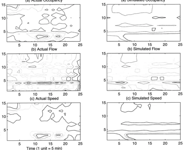
The time-dependent nature of the simulated values is depicted in the contour plots given in Figure 2-3. Note that in this figure the sensor stations have been numbered consecutively with sensor 15 as 1 and sensor 3 as 15 (See Figure 2-1). The plots are drawn with time on the X-axis and the sensor numbers on the Y-axis. Each time unit represents 5 minutes of real time. The contours represent responses of equal value. For example, plot 2-3(a) shows the contour plot for field (plot on the left) and

23

Parameter Initial Value

cflowerbound 0.5 minresponsedistance 15 a+ 2.15 a-- 1.55 -1.67 1.08 1+ -0.89 IT- 1.65

simulated occupancies (plot on the right). By comparing the actual and simulated contour plots it is clear that in the field congestion builds up around sensor stations 2 and 3 and is then released, but the simulation is not able to replicate this build-up and release of congestion.

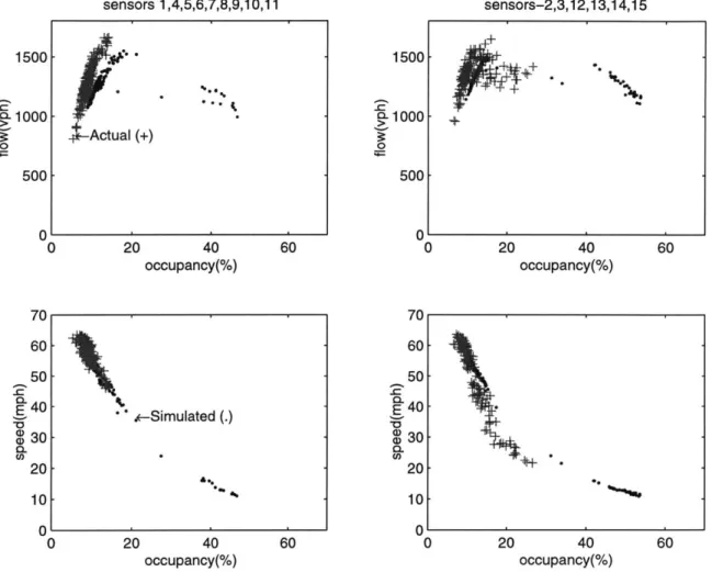
To compare the simulated and observed speed-flow-occupancy values, simulated values are drawn with a '.' and actual field data with a '+' in Figure 2-4. It was observed that in the field, the flow values at sensor stations ( 1,4,5,6,7,8,9,10,11) were on the left side of the maximum flow while congested flow was observed at sensor stations (2,3,12,13,14,15). However, as is clear from the figure, the simulated values do not show this behaviour.

From Figure 2-1 the congested flow observations correspond to the sensor lo-cations in between the Tennyson on/off-ramps and the sensors in between the A street on-ramp and Hesperian off-ramp. From the speed-occupancy plots shown in Figure 2-4 it is clear that the simulated and observed speed-occupancy plots show substantial difference. As discussed in section 2.1.1 May and Keller [18] showed that by varying the car-following parameter values different speed-occupancy relations can be obtained. Hence, we would expect that the calibration procedure adopted namely, calibrating the car-following model parameters would better simulate the speed-occupancy relationship and the build-up and dissipation of congestion.

2.4

Conclusion

We discussed the microscopic traffic simulator-MITSIM and identified the car-following model parameters for calibration. The range of values for these parameters were also determined. The network under study was discussed and the field data was compared to the simulated data. The next chapter discusses the first step in the calibration process, namely, selecting a sub-set of parameter from the eight parame-ters (cflowerbound, minresponsedistance, a+, a-,

#+,

/-- y+, 7-) that we identified in this chapter.

(a) Flow(vph) oTJ 0 0 0 Cr (ID CD% Cb 60 40 20 0 0 500 1000 1500 Actual (b) Speed(mph) / ' *.--. /a (c) Occupancy(%) 30 Co E 20 10 0 0 20 40 60 Actual 0 10 20 30 Actual Co Cl) E E 1500 1000 500 .- -/ - /. - -

-(a) Actual Occupancy ...- .... 5 10 15 20 2~ (b) Actual Flow vi, " C 5 10 15 (c) Actual Speed 15

(a) Simulated Occupancy (.- 10-5 5 15 10 5 20 25 15 5 10 15 20 2 (b) Simulated Flow 5 10 15 20 2 (c) Simulated Speed 101 5 5 10 15 20 25

Time (1 unit = 5 min)

5 10 15 20 25

Figure 2-3: Contour plots of simulated and field data.

15 10 5 15 10 5 15 (I) .0 E 10 z 0 a5 5 5

sensors-2,3,12,13,14,15 20 40 60 occupancy(%) -C 0 1500 1000. 500 0 70 60 50( E 4( 0 30 2(0 1C f 20 40 60 occupancy(%) 0 20 40 60 occupancy(%) 0 20 40 60 occupancy(%)

Figure 2-4: Comparison of simulated and field data

27 1500- 0-1000- 500-0 -0 + 70 60 50 C-E40 a)03₃₀ 20 10 0 0 i. -Simulated ()-sensors 1,4,5,6,7,8,9,10,11

Chapter 3

Sensitivity Analysis

It was pointed out in the previous chapter that a single simulation run, of the network

under consideration, takes more than twenty minutes of simulation time. Even after selecting the car-following model for calibration, we were left with eight parameters. It

would be advantageous to still reduce the number of parameters and calibrate only the

sensitive ones. Experimental design is a common methodology used to determine the sensitivity with respect to the given parameters with the least number of simulation

runs.

In experimental design, the input parameters are called factors and the output performance measures are called responses. In our study, the simulation was the ex-periment, and the input parameters were the factors. Since minimizing the deviation between the simulated and actual observations was our goal, we considered different quantitative performance measures (responses) to select the 'best' among them. For a given response, the most sensitive parameters were determined using experimental design techniques.

This chapter discusses a few performance measures (responses) used, a common experimental design technique, and how the set of sensitive parameters were identified using this technique.

3.1

Responses

As discussed earlier, we need quantitative performance measures (responses) for con-ducting a successful experimental design. Since we had three output measures, namely flow, speed, and occupancy, we used separate performance measures for each of them. In literature, it is a common methodology to use the sum of squares of the deviations as a performance measure. Based on this the following performance measures were suggested.

low (siulatedflow - actualflow)2

allsensors alltime

Ospeed E

Z

(simulatedspeed - actualspeed)2

allsensors alltime

boccupancy =

Z

E (simulatedoccupancy - actualoccupancy)

2

allsensors alltime

The three responses were selected for their simplicity. Note that each response corresponds to an output measure of interest. An important question had to be answered using the three different responses. If the sensitivity study showed that the sensitive parameters for the three responses were the same, then minimization of one response measure will affect the others. However, if the sensitive parameters were different, then each response can be calibrated separately.

The sensitive parameters were determined using experimental design methodology and the next section discusses the experimental design technique.

3.2

Experimental Design

If a simulation model has only one factor, then experimental design is simple: we just need to run the simulation at various values, or levels, of the factor and from the analysis of the responses, a conclusion can be made as to whether the factor is sensitive or not. However, if there is more than one factor (say k factors), then we also have to take into account the interactions between the factors, i.e. whether the effect of one factor depends on the level of other factors. One way to measure the effect of a particular factor would be to keep the level of all the other k-1 factors

Table 3.1: Design matrix for a 23 factorial design

fixed and vary the level of the factor of interest and see how the response changes. The whole process can be repeated for all the other factors. Such a process is not only inefficient but it also does not allow us to measure the interactions between the factors. A more efficient strategy is to use factorial experimental design techniques to decide on a systematic way of performing experiments at different factor levels, so that sufficient information can be gathered to identify the sensitive factors and their interactions.

3.2.1 2k Factorial Design

In a 2k factorial design, we choose two levels for each factor and then simulations are

done for each of the 2k possible factor-level combinations, which are also called design points. The form of the simulation experiments can be represented in a compact tabular form, also known as a design matrix, as shown in Table 3.1, for three factors

(k=3). The '-' sign is associated with one level of a factor and the '+' sign represents

the other. Since there are three factors, we have 23 = 8 possible design points. The variables Ri for i=1,2,...,8 are the values for the response when running the simulation with the ith combination of the factor levels.

Typically, we are interested in two kinds of effects: the main and interaction effects. The main effect measures how each factor individually affects the response and the interaction effect measures whether the effect of one factor depends on the

Design Point Factor-1 Factor-2 Factor-3 Response

1 - - - R1 2 + - -R2 3 + -R3 4 + + - R4 5 + R5 6 + - + _R6 7 -+ + R7 8 + + + R8

level of other factors. It is easy to calculate the main and interaction effects from the design matrix.

The main effect of factor

j

is the average change in the response due to moving the factor

j

from its '-' level to its '+' level while holding all the other factors fixed. This average is taken over all the combinations of the other factor levels in the design. From Table 3.1 the main effect of factor 1 (e1) is thus

(R2 A- R1) +(R4 ei - R3)+ (R6 -= R5)+(R A- R7)(31 (3.1) 4

and for factor 2 is

e R3 - - R1) +(R4 - R2) +(R7 - R5)+ (R8 - R6)(.2

= _(3.2)

From Table 3.1 and the equations 3.1 and 3.2 a simple formula for the main effect can be devised. To compute ej we simply apply the signs in the 'Factor-j' column to the corresponding Ri, add them up, and then divide by 2 -1.

The interactions are measured using interaction effects. For a 3 factor design, we have two-factor and three-factor interaction effects. Again an expression for in-teraction effects can be easily determined from the design matrix. To compute eij (two-factor i-j interaction), for each row, we multiply the sign in the 'Factor-i' col-umn with the sign in the 'Factor-j' colcol-umn, with the convention that the product of

like signs is a '+' and the product of opposite signs is a '-'. We apply this sign to

the corresponding Ri and add them up and divide by 2 -1. Using this formula the interaction effect e13 can be written as follows.

AR - R2)+ (R3 - R4)+ (R6 - R5)+ (R8- R7)

e13 =

A similar formula can also be devised for determining the three-factor interaction effect e₁₂₃

-A - R1)+R3 -R4)+(R5- R6)+ (R8- R7)

e123=4

Note that the effects are symmetric; for example e₁₂ = e21, e13 = e31, etc. and also

-123 = e-231 = e3 12, etc.

3.2.2

Fractional Factorial Designs

In the previous section, an experimental design with three factors was examined. In more involved designs, a large number of factors would be present and the number of design points would become quite large; a design with 8 factors will involve 28 = 256 design points. Hence, when the number of factors are large, a full factorial design is not practical. However, there are a few procedures that can be used to screen out unimportant factors.

Fractional factorial design provides a way to get good estimates of the main effects and two-way interactions at a fraction of the computational effort required by a full

2k factorial design. In a fractional factorial design, we choose a subset (of size 2k-p

where 0 < p < k) from the 2k design points and run simulations for only these chosen points. If p is large, the number of runs is less, but we would get less information from the design. The information loss is understood in terms of confounding in 2k-p designs. Since we are reducing the number of design points, it could happen that the formulas for two effects are the same. In this case the effects are said to be confounded with each other.

Resolution is the term used to quantify the effect of confounding in 2k-p factorial

designs. In a fractional factorial design, it is guaranteed that two effects are not con-founded with each other if the sum of their 'ways' is less than the designs resolution; for this purpose the main effects are regarded as 'one-way' effects. For instance in a resolution IV (resolution four) design the main effects are not confounded with two-way interactions ( 1 + 2 < 4 ), but the two-way interactions are confounded with each other (2 + 2 = 4). Thus, resolution IV design allows us to obtain main effects but cannot provide reliable two-way effects. A resolution V design on the other hand allows us to obtain main and two-way effects, but three-way effects will be confounded with two-way effects.

design points (i.e p in 2k-P) has to be determined. The design matrix, for a given

number of factors and desired resolution, can be obtained from experimental design literature [17].

3.2.3

Response Functions

A simulation model can be considered as a function with the responses depending on the input parameters. The form of the function is unknown, and response function methodology is a method used to approximate this function. Depending on the res-olution of the experimental design technique, different functional forms can be fitted to the responses 3.3. The coefficents of the response funtion are usually estimated using least-square regression. Fatorial designs, are actually based on regression meta-models and the regression least-square estimates are related to the effects estimates in experimental design. Note that if we are considering a two factorial design, since a variables has only two levels, the response function as given in 3.3 can be equivalently represented and estimated using a dummy variable for each parameter.

The methodology we followed, to find the sensitive parameters, was to first fit a polynomial function, with single order and all the two-factor interaction terms, to the response. Then the influence of each term on the response variation was analyzed,

and less significant ones were dropped in the final model. Thus, the final model had only the most significant parameters.

3.2.4

Stochasticity

Since we were dealing with a stochastic simulator, we had to replicate the simulation at each design point. The simulation was replicated five times at each design point (See Appendix C), and the response function was fitted to the average values of the responses over the five replications.

3.3

Results

A fractional factorial design of resolution five: 2y was conducted for the eight pa-rameters identified in Chapter 2. The design matrix is given in Table 3.2. For each design point, the three responses as given in Section 3.1 were evaluated. The plot of the responses versus the iterations is shown in Figure 3-1. From this figure it is not evident whether the three responses are sensitive to the same set of parameters.

To determine this, each response was initially represented by a polynomial func-tion, with all the one-way and two-way interaction effects. The form of the response function is given in 3.3

8 8 8

R = ip + E#ixi +

E

> #ijzixj (3.3)

i=1 i=1,i<j j=1

where p is the constant and R is the response.

x1 represents the variable minrespdistance, x2 is cflowerbound, x3 is a+, x4 is /#+,

X5 is 'Y+, x6 is C, x7 is

#_,

and x8 is ..

The

#

are the coefficients to be determined from the analysis.

Finally the influence of each term on the response was analyzed and less significant ones were dropped in the final model

As an example consider the response function given by

$O =

S

E (simulated pow - actualf po )2

allsensors alltime

The response is approximated as shown in Equation 3.3. The first step in determining the sensitive variables is to screen out the less sensitive variables. For this, an analysis of variance is conducted and the influence of each term on the response variation is analyzed. The result of such an analysis using the BOSS/Quatro software program (See Appendix A) is given in Table 3.3

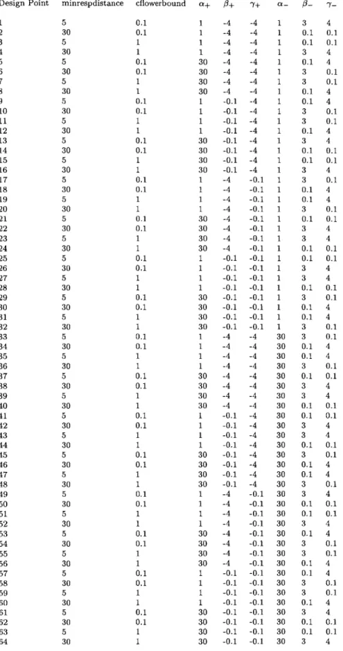
Each row in Table 3.3 represents a term in Equation 3.3. The SOURCES column represents the variables. As shown in Equation 3.3 we have eight variables, they are represented by the rows from 1 to 8. The next set of rows represent the two-way

Design Point minrespdistance 1 5 0.1 1 -4 -4 1 3 4 2 30 0.1 1 -4 -4 1 0.1 0.1 3 5 1 1 -4 -4 1 0.1 0.1 4 30 1 1 -4 -4 1 3 4 5 5 0.1 30 -4 -4 1 0.1 4 6 30 0.1 30 -4 -4 1 3 0.1 7 5 1 30 -4 -4 1 3 0.1 8 30 1 30 -4 -4 1 0.1 4 9 5 0.1 1 -0.1 -4 1 0.1 4 10 30 0.1 1 -0.1 -4 1 3 0.1 11 5 1 1 -0.1 -4 1 3 0.1 12 30 1 1 -0.1 -4 1 0.1 4 13 5 0.1 30 -0.1 -4 1 3 4 14 30 0.1 30 -0.1 -4 1 0.1 0.1 15 5 1 30 -0.1 -4 1 0.1 0.1 16 30 1 30 -0.1 -4 1 3 4 17 5 0.1 1 -4 -0.1 1 3 0.1 18 30 0.1 1 -4 -0.1 1 0.1 4 19 5 1 1 -4 -0.1 1 0.1 4 20 30 1 1 -4 -0.1 1 3 0.1 21 5 0.1 30 -4 -0.1 1 0.1 0.1 22 30 0.1 30 -4 -0.1 1 3 4 23 5 1 30 -4 -0.1 1 3 4 24 30 1 30 -4 -0.1 1 0.1 0.1 25 5 0.1 1 -0.1 -0.1 1 0.1 0.1 26 30 0.1 1 -0.1 -0.1 1 3 4 27 5 1 1 -0.1 -0.1 1 3 4 28 30 1 1 -0.1 -0.1 1 0.1 0.1 29 5 0.1 30 -0.1 -0.1 1 3 0.1 30 30 0.1 30 -0.1 -0.1 1 0.1 4 31 5 1 30 -0.1 -0.1 1 0.1 4 32 30 1 30 -0.1 -0.1 1 3 0.1 33 5 0.1 1 -4 -4 30 3 0.1 34 30 0.1 1 -4 -4 30 0.1 4 35 5 1 1 -4 -4 30 0.1 4 36 30 1 1 -4 -4 30 3 0.1 37 5 0.1 30 -4 -4 30 0.1 0.1 38 30 0.1 30 -4 -4 30 3 4 39 5 1 30 -4 -4 30 3 4 40 30 1 30 -4 -4 30 0.1 0.1 41 5 0.1 1 -0.1 -4 30 0.1 0.1 42 30 0.1 1 -0.1 -4 30 3 4 43 5 1 1 -0.1 -4 30 3 4 44 30 1 1 -0.1 -4 30 0.1 0.1 45 5 0.1 30 -0.1 -4 30 3 0.1 46 30 0.1 30 -0.1 -4 30 0.1 4 47 5 1 30 -0.1 -4 30 0.1 4 48 30 1 30 -0.1 -4 30 3 0.1 49 5 0.1 1 -4 -0.1 30 3 4 50 30 0.1 1 -4 -0.1 30 0.1 0.1 51 5 1 1 -4 -0.1 30 0.1 0.1 52 30 1 1 -4 -0.1 30 3 4 53 5 0.1 30 -4 -0.1 30 0.1 4 54 30 0.1 30 -4 -0.1 30 3 0.1 55 5 1 30 -4 -0.1 30 3 0.1 56 30 1 30 -4 -0.1 30 0.1 4 57 5 0.1 1 -0.1 -0.1 30 0.1 4 58 30 0.1 1 -0.1 -0.1 30 3 0.1 59 5 1 1 -0.1 -0.1 30 3 0.1 60 30 1 1 -0.1 -0.1 30 0.1 4 61 5 0.1 30 -0.1 -0.1 30 3 4 62 30 0.1 30 -0.1 -0.1 30 0.1 0.1 63 5 1 30 -0.1 -0.1 30 0.1 0.1 64 30 1 30 -0.1 -0.1 30 3 4

Table 3.2: Design matrix for a 2 8 factorial design 35

x 108 21 1.5-0.5 -' -0 10 20 30 40 50 60 x 10 6 6 * . * .04-2 --010 20 30 40 50 60 5 X 105 Io 1 -* 0 10 20 30 40 50 60 design point

interaction effects. For example, the ninth row with numbers 1 2 under the sources column represent the two-way interaction between the variables x1 and x2. Since we

have eight variables we have a total of 8C2 = 28 two-way interaction effects. The

SUM OF SQUARES column gives the variation due to each variable. The residual variation is given in the second to last row, and the total variation is given in the last row. DF denotes the degree of freedom. MEAN SQUARED is an estimate of the variance. The residual mean squared is also given in the second to last row. The column F-LEVEL gives the result of the F-test: for each variable the ratio of its mean squared to the residual mean squared. Based on the F-test a conclusion is made as to a variable's significance.

We can see that the main effect of only a few parameters are significant. Also note that the interaction effects are significant only for those parameters with significant main effects. So, in the next step, the response function is modified to include only the significant terms, and the analysis is done again. The result is shown in Table

3.4. The same procedure is applied to the response 4 _{speed and}

/occupancy. The results for the final model are shown in Tables 3.5 and 3.6.

3.4

Conclusion

We can see that the four parameters (cflowerbound, a-, /-, -y) (see Chapter 2) were found to be sensitive for the three responses. Moreover, these four parameters affect the deceleration characteristics of a vehicle. It appears that the parameters affecting the deceleration characteristics are more sensitive to the current data set. Also note that since the sensitive parameters were found to be the same for the three responses, the minimization of one response will definitely affect others.

The results obtained depends on the range and levels of the parameters. The range of the paramater values should be correctly determined . As discussed in section 2.2.1 the values we used were based on previous estimation studies. Moreover, when we use a 2k factorial design, we are assuming that the parameter effects vary linearly

between the '+' and '-' values. This could be improved by using a 3 k factorial design,

though with increased computational costs.

The next chapter discusses the calibration of these parameters over the range of values determined in Chapter 2.

ANALYSIS OF VARIANCE

SOURCES SUM OF SQUARES DF. MEAN SQUARED F-LEVEL CONCLUSION

0.1677211E+14 0.6921709E+16 0.1128680E+14 0.1963264E+15 0.1371702E+15 0.1382006E+17 0.4448516E+17 0.1105315E+18 0.3015633E+14 0.7470733E+13 0.1449746E+13 0.9150158E+14 0.2347503E+11 0.1427141E+14 0.1352122E+14 0.4943016E+12 0.2385160E+14 0.2293346E+14 0.3730828E+15 0.4156797E+16 0.1148690E+14 0.1171587E+14 0.2205883E+13 0.4250261E+13 0.1626635E+13 0.1626996E+14 0.1655424E+15 0.3419700E+13 0.3463867E+10 0.3454109E+13 0.9820832E+13 0.1073757E+14 0.1830763E+12 0.9438494E+16 0.1109459E+17 0.1358164E+17 0.1400204E+17 0.229213E+18 27 63 0.167721E+14 0.692171E+16 0.112868E+14 0.196326E+15 0.137170E+15 0.138201E+17 0.444852E+17 0.110531E+18 0.301563E+14 0.747073E+13 0.144975E+13 0.915016E+14 0.234750E+11 0.142714E+14 0.135212E+14 0.494302E+12 0.238516E+14 0.229335E+14 0.373083E+15 0.415680E+16 0.114869E+14 0.117159E+14 0.220588E+13 0.425026E+13 0.162663E+13 0.162700E+14 0.165542E+15 0.341970E+13 0.346387E+10 0.345411E+13 0.982083E+13 0.107376E+14 0.183076E+12 0.943849E+16 0.110946E+17 0.135816E+17 0.518594E+15 0.323415E-01 0.133471E+02 0.217642E-01 0.378574E+00 0.264504E+00 0.266491E+02 0.857803E+02 0.213137E+03 0.581502E-01 0.144057E-01 0.279553E-02 0.176442E+00 0.452667E-04 0.275194E-01 0.260729E-01 0.953157E-03 0.459928E-01 0.442224E-01 0.719412E+00 0.801551E+01 0.221501E-01 0.225916E-01 0.425359E-02 0.819574E-02 0.313663E-02 0.313732E-01 0.319214E+00 0.659418E-02 0.667934E-05 0.666053E-02 0.189374E-01 0.207052E-01 0.353024E-03 0.182002E+02 0.213936E+02 0.261894E+02 NO SIGNIFICANT HIGH. SIGNIFICANT NO SIGNIFICANT NO SIGNIFICANT NO SIGNIFICANT HIGH. SIGNIFICANT HIGH. SIGNIFICANT HIGH. SIGNIFICANT NO SIGNIFICANT NO SIGNIFICANT NO SIGNIFICANT NO SIGNIFICANT NO SIGNIFICANT NO SIGNIFICANT NO SIGNIFICANT NO SIGNIFICANT NO SIGNIFICANT NO SIGNIFICANT NO SIGNIFICANT HIGH. SIGNIFICANT NO SIGNIFICANT NO SIGNIFICANT NO SIGNIFICANT NO SIGNIFICANT NO SIGNIFICANT NO SIGNIFICANT NO SIGNIFICANT NO SIGNIFICANT NO SIGNIFICANT NO SIGNIFICANT NO SIGNIFICANT NO SIGNIFICANT NO SIGNIFICANT HIGH. SIGNIFICANT HIGH. SIGNIFICANT HIGH. SIGNIFICANT

Table 3.3: Screening for o4_f,, Residual