Calibration of strapdown system accelerometer dynamic errors

CALIBRATION OF STRAPDOWN SYSTEM

ACCELEROMETER DYNAMIC ERRORS

by

Richard Lee Needham, Jr.

B.S., Aerospace Engineering, United States Naval Academy Annapolis, Maryland (1992)

Submitted to the Department of Aeronautics and Astronautics in Partial Fulfillment of the Requirements for the Degree of MASTER OF SCIENCE IN AERONAUTICS AND ASTRONAUTICS

at the

MASSACHUSETTS INSTITUTE OF TECHNOLOGY

June 1994

© Richard Lee Needham, Jr., 1994. All Rights Reserved

/' /A

Signature of Author

Certified by

Certified by

Accepted by

Department of Aeronautis and Astronautics

/ ,. 13 May 1994

Professor Wallace E. Vander Velde Department of Aeronautics and Astronautics Thesis Advisor

Tom P. Thorvaldsen ) Charles Stark Draper Laboratory, Inc. Technical Supervisor

Professor Harold Y. Wachman Chairman, Department Graduate Committee

MASSACHUSETTS _INSTITUTE OF TFriJi11llM

U8AR~Es

Aero

CALIBRATION OF STRAPDOWN SYSTEM ACCELEROMETER DYNAMIC ERRORS

by

Richard Lee Needham, Jr.

Submitted to the

Department of Aeronautics and Astronautics on May 13, 1994.

In Partial Fulfillment of the Requirements for the Degree of Master of Science in Aeronautics and Astronautics

Abstract

The calibration of the error terms in strapdown system accelerometers due to angular motion is performed using a three-axis gimbaled test table simulation. The sensitivities of the accelerometers to angular velocities and angular accelerations are reduced to accelerometer error coefficients so that a linear estimation can be performed. Linear covariance analysis, using a square root Kalman filter, is used to predict the error dynamics for the simulation.

Various test table gimbal trajectories are implemented to reduce the errors in the accelerometer coefficients. The effects of increasing either the sensitivities or the observabilities of the accelerometer coefficients are compared. The time the gimbals are held at their maximum rates and the initial gimbal angles are varied to observe their effects on the resulting errors in the accelerometer error coefficients. The effects of the displacements between the gimbal axes of the test table are also investigated and shown to be small. The performances of all the trajectories are compared to a previously existing trajectory, resulting in errors that are up to 87.8% lower. The best trajectory found in this research is one that is locally optimized over three trajectory characteristics.

Thesis Advisor: Professor Wallace E. Vander Velde Professor of Aeronautics and Astronautics Technical Supervisor: Tom P. Thorvaldsen

Principal Member Technical Staff

Acknowledgments

I would like to express my sincere appreciation to all those who helped me throughout my research effort. Primary thanks go to my technical supervisor, Tom P. Thorvaldsen, who provided the initial idea for this research. His tireless support and guidance were instrumental in developing and completing this thesis. He also managed to squeeze in a few late nights, providing invaluable help when I needed it most. I would also like to extend my deepest gratitude to Professor Wallace E. Vander Velde, who always kept me focused and provided new insights. His ability to describe complex ideas in a clear, concise manner helped me both in the classroom and in the most difficult parts of this research.

I would also like to express my thanks to the Charles Stark Draper Laboratory for making my studies at MIT possible. Thanks go to the technical staff of the Guidance and Navigation Analysis Division, including Tony Bogner, Darold Riegsecker, and Howie Musoff, for providing invaluable technical support and assistance. Although I learned much in the classroom, I learned just as much from my officemates and friends at the lab. Matt and Chris both helped me along the way and made my experience here not only a learning one, but an enjoyable one. Jeff was also always there, providing me with technical help, financial advice, and friendship.

I would like to thank my parents, for without them I never would have made it this far. They have taught me that anything is possible, and that no matter what I decide to do, they will support me in every way. I cannot express how much I appreciate their constant love and support.

Finally, I would like to thank Deborah. She has made the past year and a half one of the happiest times in my life. Her thoughtfulness, patience, and love have meant more to me than she will ever know.

This thesis was researched and written at the Charles Stark Draper Laboratory under the Navy RIMU-S CONTINUATION Project, Contract N00030-93-G-0074-EK08.

Publication of this thesis does not constitute approval by the Charles Stark Draper Laboratory or the United States Navy of the findings or conclusions contained herein. It is published for the exchange and stimulation of ideas.

I hereby assign my copyright of this thesis to the Charles Stark Draper Laboratory, Inc., of Cambridge, Massachusetts.

Richard L. Neddiam, Jr. 6

May 13, 1994

Permission is hereby granted by the Charles Stark Draper Laboratory, Inc. to the Massachusetts Institute of Technology to reproduce and to distribute copies of this thesis document in whole or in part.

Table of Contents

Description Page

List of Figures ... 10

List of Tables ... 13

List of Sym bols ... 14

Chapter 1: Introduction ... 17

1.1 Background and Motivation ... ... 17

1.2 Inertial Navigation Systems ... 18

1.2.1 Basic Inertial Navigation Systems ... 18

1.2.1.1 Gimbaled Systems vs. Strapdown Systems ... 20

1.2.2 Accelerometer Structure ... ... 20

1.2.3 Errors in Accelerometers ... ... 23

1.2.3.1 Static Errors ... 24

1.2.3.2 Angular Motion Errors ... ... 26

1.2.3.3 Testing Errors ... ... 27

1.2.4 Error Terms Calibrated in This Thesis ... 28

1.3 Previous Work ... 28

Chapter 2: Analytic Development ... 31

2.1 Accelerometer Error Model ... 31

2.1.1 Assumptions on Previously Calibrated Quantities ... 31

2.1.2 Angular Effects on Accelerometer Output ... 32

2.1.2.1 Angular Velocity Sensitivity ... 32

2.1.2.2 Angular Acceleration Sensitivity ... 35

2.1.2.3 Total Sensitivity to Angular Motion in Accelerometer Frame ... 37

2.1.3 Reduction of Parameters into Angular Dependent Coefficients ... 39

2.2 Simulation Model ... 42

2.2.1 Test Table ... ... 43

2.2.2 Navigator Position ... ... 44

2.2.2.1 Gimbal Axis Displacements ... 44

2.3 Measurements and the Kalman Filter ... 47

2.3.1 Covariance Analysis ... 48

2.3.2 States and Dynamics Equation ... 48

2.3.3 Modeling Noise ... 51

2.3.4 Measurements and Measurement Equation ... 52

2.3.4.1 Measurement Noise ... 53

2.3.5 Filter Propagation and Update Equations ... 54

2.3.5.1 Square Root Filter Implementation ... 55

2.3.5.2 Propagation of Covariance Matrix ... 56

Chapter 3: Implementation ... 59

3.1 Initial Assumptions ... 59

3.1.1 Initial Covariance ... 59

3.1.2 Test Table Setup ... ... 61

3.1.2.1 Type and Geometry of Table ... 61

3.1.2.2 Table Constraints ... 62

3.1.2.3 Table Accuracies ... 63

3.2 Initial Trajectories ... 64

3.2.1 Previous Trajectory ... 64

3.2.1.1 Testing Time Modifications ... 68

3.2.2 Heuristic Trajectories ... 69

3.3 Improved Trajectories ... ... 74

3.3.1 Objective of Improved Trajectories ... 74

3.3.2 Effects of Small Changes in Characteristics of Trajectory ... 75

3.3.2.1 Time at Maximum Rate ... 75

3.3.2.2 Initial Angles ... 76

3.3.3 Maximizing Body Frame Angular Rates and Angular Accelerations ... 77

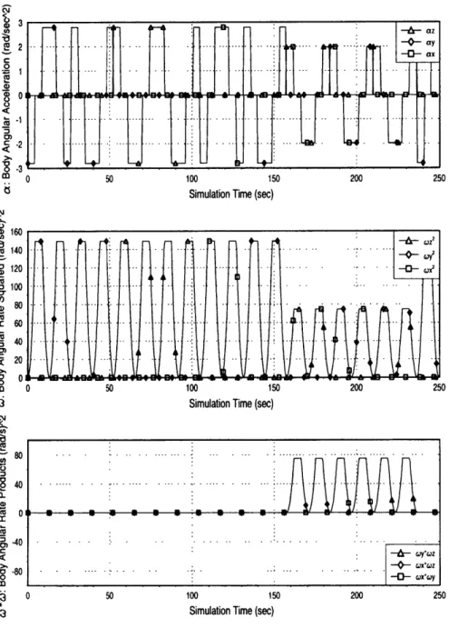
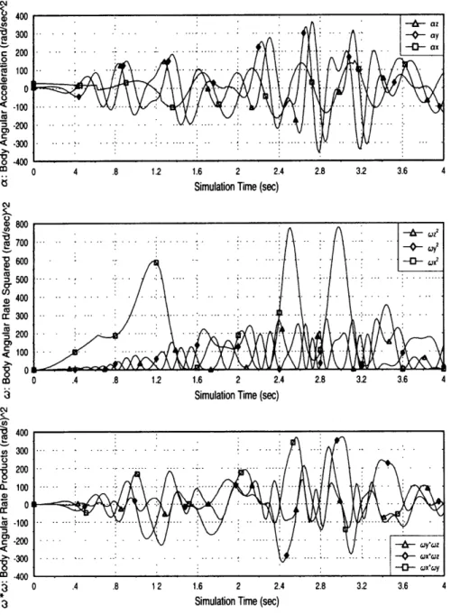
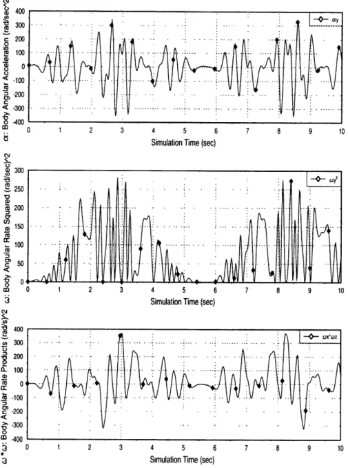
3.3.3.1 Sensitivities to Body Angular Accelerations ... 78

3.3.3.2 Sensitivities to Squares of Body Angular Velocities ... 82

3.3.3.3 Sensitivities to Products of Body Angular Velocities ... 84

3.3.4 Use of Extended Trajectories ... 87

C hapter 4: R esults ... ... 91

4.1 Initial Trajectories ... ... . ... 92

4.1.1 Previous Trajectory ... 92

4.1.2 Initial Heuristic Trajectories ... 97

4.2 Trajectory Characteristic Effects ... 100

4.2.1 Time at Maximum Rate Effects ... 102

4.2.3 Summary of Trajectory Characteristic Effects ... 108

4.3 Extended Trajectories ... 109

4.3.1 Full Extended Trajectories ... 109

4.3.2 Extended Initial Trajectories ... 114

4.3.3 Summary of Extended Trajectories ... 116

4.4 Modeling Effects ... 116

4.4.1 Runge Kutta Integration Step Size Effects ... 117

4.4.2 Measurement Frequency Effects ... 117

4.4.3 Incorporation of Gimbal Axis Displacements ... 118

4.5 General Error Estimation Trends ... 121

4.5.1 Summary of Results ... 121

4.5.2 Position and Velocity Errors ... 124

4.5.3 Worst Coefficient Estimates ... 124

Chapter 5: Conclusions ... ... 127

5.1 Summary ... ... 127

5.2 Proposed Future Work ... 129

Appendix A: Test Table Gimbal Trajectories ... .... 131

Appendix B: Graphical Results ... 157

Appendix C: Gimbal to Body Transformations ... 175

Appendix D: Square Root Filter ... ... 181

List of Figures

Figure 1.1 : Pendulous Accelerometer Structure ... Figure 1.2 : Simplified Pendulous Accelerometer Cross Section ... Figure 1.3 : Null Offset Error Mechanism ... ... Figure 2.1 : Angular Velocity Acting on Accelerometer ... Figure 2.2 : Misalignment of Pendulum Axes About Case Axes ... Figure 2.3 : Orientation of Individual Accelerometer Axes to Case Axes ... Figure 2.4 : Three-Axis Gimbal Test Table ... .... Figure 2.5 : Middle Gimbal Origin in Outer Gimbal Frame ... Figure 2.6 : Inner Gimbal Origin in Middle Gimbal Frame ... Figure 3.1 : GTO Gimbal Trajectory ... ... Figure 3.2 : GTO Body Frame Sensitivities ... Figure 3.3 : GTI Gimbal Trajectory ... ... Figure 3.4 : Representative GT1 Body Frame Sensitivities ... Figure 4.1 : X Accelerometer Coefficient Errors for GTO ... Figure 4.2 : Y Accelerometer Coefficient Errors for GTO ... Figure 4.3 : Z Accelerometer Coefficient Errors for GTO ... Figure 4.4 : Representative GT 1 Body Frame Y-Axis Sensitivities ... Figure 4.5 : Representative GT3 Body Frame Y-Axis Sensitivities ... Figure 4.6: Y Accelerometer Coefficient Errors for GT1 ... Figure 4.7 : Holding Period Effects on Final Cost ... ... ... .... Figure 4.8 : Initial Middle Gimbal Angle Effects on Final Cost ... Figure 4.9 : Initial Inner Gimbal Angle Effects on Final Cost ... Figure 4.10 : Z Accelerometer Coefficient Errors for GT6 ... Figure 4.11 : Z Accelerometer Coefficient Errors for GT6b ... Figure 4.12 : Z Accelerometer Coefficient Errors for GT6c ... Figure 4.13 : Extra Cost Due to Gimbal Axis Displacements for GTO ... Figure 4.14 : Extra Cost Due to Gimbal Axis Displacements for GT3 ... Figure A.1 : GTO Gimbal Trajectory ... ... Figure A.2: GTI Gimbal Trajectory ... ... Figure A.3 : GT2 Gimbal Trajectory ... ... Figure A.4 : GT3 Gimbal Trajectory ... ... Figure A.5 : GT4 Gimbal Trajectory ... ...

Page 21 23 25 32 38 40 43 45 46 66 67 71 73 94 95 96 98 99 101 104 106 107 111 112 113 119 120 132 133 134 135 136

Figure A.6: Figure A.7 : Figure A.8 : Figure A.9: Figure A. 10 Figure A. 11 Figure A.12 Figure A.13 Figure A. 14 Figure A. 15 Figure A. 16 Figure A. 17 Figure A. 18 Figure A. 19 Figure A.20 Figure A.21 Figure A.22 Figure A.23 Figure A.24 Figure A.25 Figure B.1 : Figure B.2: Figure B.3 : Figure B.4 : Figure B.5 : Figure B.6 : Figure B.7 : Figure B.8 : Figure B.9: Figure B.10 Figure B. 11 Figure B.12 Figure B. 13 Figure B.14 Figure B.15 Figure B.16 GT5 Gimbal Trajectory ... ... GTX 1 Extended Gimbal Trajectory ... GTX Ib Extended Gimbal Trajectory ... .... GTX2 Extended Gimbal Trajectory ... : GTX2b Extended Gimbal Trajectory ... : GTX3 Extended Gimbal Trajectory ... : GTX3b Extended Gimbal Trajectory ...

: GTX4 Extended Gimbal Trajectory ... : GTX5 Extended Gimbal Trajectory ... : GTX6 Extended Gimbal Trajectory ...

: GTX7 Extended Gimbal Trajectory ... : GTX7b Extended Gimbal Trajectory ... : GTX8b Extended Gimbal Trajectory ... : GTX9 Extended Gimbal Trajectory ... : GT6 Gimbal Trajectory ... ... : GT6b Gimbal Trajectory ... : GT6c Gimbal Trajectory ... ... : GT3opt Gimbal Trajectory ... ...

: GT4x Gimbal Trajectory ... : GT7 Gimbal Trajectory ... ... GT6 Body Frame X-Axis Sensitivities ... GT6 Body Frame Y-Axis Sensitivities ... GT6 Body Frame Z-Axis Sensitivities ... GT6b Body Frame Sensitivities ...

Cost Function for GTO ... ... Cost Function for Initial Heuristic Trajectories ... Cost Function for GT4 and GT5 Trajectories ... Holding Time Effects on Cost Function ... Initial Middle Gimbal Angle Effects on Cost Function ... : Initial Inner Gimbal Angle Effects on Cost Function ... : Cost Function for Full Extended Trajectories ... : Cost Function for Extended Initial Trajectories ...

: Runge Kutta Step Size Effects on Cost Function ... : Measurement Frequency Effects on Cost Function ... : Gimbal Axis Displacement Effects on Cost Function for GT3 ... : Gimbal Axis Displacement Errors vs. Time for GTI ...

137 138 139 140 141 142 143 144 145 146 147 148 149 150 151 152 153 154 155 156 158 159 160 161 162 163 164 165 166 167 168 169 170 171 172 173

Figure B. 17 : Position and Velocity Errors for GT I vs. Time ... 174 Figure C. 1 : Local Level Frame to Body Frame (3-2-1) Transformation ... 175

List of Tables

Description Page

Table 2.1 : Accelerometer Axes to Accelerometer Case Axes Relations ... 40

Table 2.2a: X-Accelerometer Error Coefficients ... . 41

Table 2.2b : Y-Accelerometer Error Coefficients ... . 41

Table 2.2c : Z-Accelerometer Error Coefficients ... 42

Table 3.1 : Initial Standard Deviations ... 60

Table 3.2 : Initial Accelerometer Coefficient Standard Deviations (Inches) ... 61

Table 3.3 : Test Table Constraints ... 63

Table 3.4 : Test Table Performance Specifications ... 64

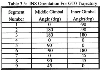
Table 3.5 : INS Orientation for GTO Trajectory ... 65

Table 3.6 : Testing Time Modifications to Previous Trajectory ... 68

Table 3.7 : Extended Trajectory Gimbal Accelerations, Velocities, and Angles ... 88

Table 3.8 : Segment Orders for GT6b and GT6c ... 90

Table 4.1 : Effects of Successive One-Dimensional Optimizations on Final Cost ... 108

Table 4.2 : Final Costs for All Basic Trajectories ... 121

Table 4.3 : Final Costs for Variations in Holding Times in GT3 Trajectory ... 122

Table 4.4 : Final Costs for Variations in Initial Middle Gimbal Angle for GT3 ... 122

List of Symbols

Symbol Description

a distance along pendulous axis from accelerometer hinge to point P

aerr,,r acceleration error

Ar', matrix relating gimbal axis displacements to rol

Aw' _{bmatrix relating gimbal rates to angular velocities in the body frame}

b distance along input axis from accelerometer hinge to point P

c distance along output axis from accelerometer hinge to point P

cl X-accelerometer error coefficient vector c2 Y-accelerometer error coefficient vector c3 Z-accelerometer error coefficient vector

Cb transformation matrix from frame a to frame b

Cij jth coefficient (1-9) of the ith accelerometer (1-3)

f, force vector acting on the ith mass element

F dynamics matrix

G sensitivity matrix of body frame acceleration errors to angular motion h measurement geometry vector

H measurement geometry matrix

I,, pendulum moment of inertia about the ith axis

I, pendulum product of inertia with respect to the i and j axes

I identity matrix

K Kalman gain matrix

l0 distance between pendulum hinge and the pendulum center of mass

m, ith mass element

M total mass of the pendulum

00 origin of the outer gimbal frame

OM origin of the middle gimbal frame

OI origin of the inner gimbal frame

P pendulosity of the pendulum

P covariance matrix

Q(t) power spectral density matrix of the process noise vector w

Qk discrete covariance matrix of process noise

r position vector

Rij distance along the jth body axis from accelerometer hinge to point P R covariance matrix of measurement noise

t time

T characteristic time period for a gimbal to reach tmx accelerating at amax

u control vector of gimbal angular accelerations

v velocity vector

vk measurement noise vector

w(t) process noise vector

Sa vector of process noise in accelerometers

r accelerometer coefficient sensitivity row vector

W square root of the covariance matrix

Xa distance from the pendulum hinge to the center of angular acceleration

X,O distance from the pendulum hinge to the center of spin

z measurement vector

Oamax maximum obtainable angular acceleration

a angular acceleration vector

l,, misalignment of the ith accelerometer about the jth case axis

aerr,,r change in acceleration error due to misalignments

ba,,,,, total acceleration error due to angular motion and misalignments

Sa, total acceleration error for the ith accelerometer

kw _{power spectral density matrix of wa} p vector of gimbal axis displacements

PM12 displacement of OI from OM along middle gimbal mg2 axis

PMi, displacement of OI from OM along middle gimbal mg3 axis

POMI displacement of OM from 00 along outer gimbal ogl axis

a, standard deviation of i

o,2 variance of i

cOmax maximum obtainable angular velocity

_o angular velocity vector

Subscript

b body frame

i inner gimbal, input axis

m middle gimbal

MI middle gimbal origin to inner gimbal origin

o outer gimbal, output axis

OI outer gimbal origin to inner gimbal origin

pendulous axis Superscript b g ig mg og p T + Operator cO E[] sO X() 3(t) Acronym GPS INS body frame

accelerometer case frame gimbal

inner gimbal frame middle gimbal frame outer gimbal frame pendulum frame transpose

estimate, unit vector

immediately after a measurement update immediately before a measurement update

cosine of 0

expected value operator sine of 0

cross product matrix operator delta function

Global Positioning System Inertial Navigation System

Chapter 1

Introduction

1.1 Background and Motivation

Many platforms that navigate using inertial navigation systems (INS's) experience some sort of angular motion. This angular motion may consist of an aircraft rolling, a spacecraft tumbling or a missile spinning. If the instruments used to measure the inertial forces are rigidly attached to the vehicle, then angular rates and angular accelerations of the vehicle will produce linear accelerations in the accelerometers. The internal characteristics of these accelerometers, as well as their placement in the vehicle, will

dictate to what extent the vehicular angular motion will affect their outputs.

Accurate navigation of ballistic missile reentry bodies is essential in determining the effect of deployment from the missile bus on the trajectory of the reentry body. For the case of ballistic missile reentry bodies, the angular motion effects on navigation are very important. When the reentry bodies are released from the missile bus they are spun up about their longitudinal axes at very high accelerations. When the reentry bodies move away from the missile bus they are spinning at very high angular rates. Deployment from the missile bus also results in forces on the reentry body that must be measured accurately in order to navigate properly. One of these forces is the impingement of the missile bus firing on the reentry body. Errors in both measured position and velocity will result if the angular motion effects on the navigation system are not compensated out. Therefore, an accurate model of the angular motion effects on the navigation system must be developed.

This thesis calibrates the error terms due to angular effects on strapdown inertial navigation system accelerometers. The INS can be mounted on a three-gimbal test table

and rotated about the three gimbal axes to measure the errors introduced through angular motion.

1.2 Inertial Navigation Systems

1.2.1 Basic Inertial Navigation Systems

An inertial navigation system (INS) is a set of instruments that allow position and velocity of a vehicle to be determined solely from internal measurements. While other navigation systems may make use of external measurements, such as radar ranging, Doppler shifts, or GPS pseudoranges, an INS merely measures the inertial angular rates and forces on the vehicle. For a properly initialized INS, these measurements can be processed to provide a continuous navigation solution. This allows the INS to navigate without any external sensors that either transmit or receive radiation (radars, lasers, radio waves, etc.).

In order for an INS to navigate, it must be capable of performing four distinct functions [1]:

* Instrument a reference frame * Measure a specific force

* Have knowledge of the gravitational field

* Time integrate the specific force data to obtain velocity and position information These functions are performed by the four basic components of any INS: three gyroscopes, three accelerometers, a gravity calculator, and an onboard digital computer used to integrate the equations of motion.

Gyroscopic instruments are used to accomplish the first function. The three gyroscopes (assumed to have a single-degree-of-freedom) can either be placed on a gimbaled platform or rigidly attached to the vehicle. If they are placed on a gimbaled platform, they define an inertially nonrotating cartesian frame. Angular motion of the vehicle about a gyros input axis will cause the gimbal supporting the spin axis to precess

about the output axis. Torques can then be applied to the gyro-supporting gimbals in order to keep the gyro spin axes pointing along the same inertial axes. This maintains an inertially stable platform in which the gyro spin axes maintain their orientation with respect to inertial space. The torques that are required to keep the gimbal supports from precessing are taken as the measurements and used to determine the orientation of the vehicle. If the gyros are rigidly attached to the vehicle, then they will no longer be nonrotating with respect to inertial space. Instead, they are used as sensing elements using a closed-loop servo system. The resulting torques applied to each gyro are then proportional to the particular gyro's inertially referenced angular velocity. The torques can be used to determine the orientation of the gyros with respect to their original orientation. Systems that use rigidly attached gyros instead of placing them on a gimbaled platform are called strapdown systems.

The second function of the INS is performed by devices called accelerometers. The accelerometers are an integral part of either gimbaled or strapdown INS's. The accelerometers are the instruments that actually measure the forces acting on the body. This is accomplished by using three orthogonal accelerometers. Each accelerometer has a proofmass that is constrained to move in one direction. When a force acts on the body, the body accelerates. If the force has a component along a particular accelerometer's input axis, then the proofmass of that accelerometer will deflect. By measuring the deflection of all the proofmasses, the acceleration magnitude and direction can be determined. Unfortunately, the accelerometer measurements also include the effects of the gravitational field. An accelerometer at rest with no external forces acting on it will read Ig down due to gravity. In order to determine the motion of the vehicle, the gravity accelerations must be removed from the accelerometer outputs. The third function of the INS is then required to accurately compensate the accelerometer outputs for the local gravity forces.

The final function of the INS, performed by an onboard navigating computer, is the integration of the measured forces. The data obtained from the accelerometers and gyros is processed, resulting in the accelerations in the inertial frame. These accelerations may then be integrated once to provide velocity information. The velocity information is then integrated once more to provide position information.

1.2.1.1 Gimbaled Systems vs. Strapdown Systems

Two forms of inertial navigation systems are the gimbaled system and the strapdown system. The difference between the two systems is the way in which the instruments are mounted on the vehicle. In gimbaled systems, the instruments maintain their orientation in an inertially nonrotating frame. In strapdown systems, the instruments are rigidly attached to the vehicle and experience the same angular motion as the vehicle.

Strapdown systems have both advantages and disadvantages over gimbaled systems. The greatest advantage of strapdown systems is their smaller size. Current systems are so small that their weight is almost negligible. Also, the power consumption for these small devices is significantly less than that of the gimbaled systems. With these advantages comes the disadvantage of a larger computational burden in computing a navigation solution. The gyro data must now be processed to determine the orientation of the vehicle with respect to an inertial frame. Also, since the instruments are rotating with the vehicle, there will be errors introduced due to angular motion. These angular motion errors are only present in strapdown systems.

1.2.2 Accelerometer Structure

There are many different ways to mechanize an accelerometer [2]. Popular designs include unbalanced cylinders, integrating unbalanced gyros, and pendulous accelerometers. One of the most common types is the pendulous accelerometer. This type of accelerometer is similar to a pendulum, consisting of a proofmass that is constrained to rotate about one axis. Accelerations experienced by the instrument are

determined by measuring the current necessary to produce a restoring torque when the pendulum deflects. The Bell XI-79 pendulous accelerometer will be used as the primary example of a strapdown system accelerometer throughout this thesis. However, all strapdown accelerometers, regardless of their design, will experience errors due to angular motion of the vehicle.

The structure of a pendulous accelerometer is shown in Figure 1.1. The ring-shaped proofmass is constrained to rotate only about the hinge (or output) axis. An acceleration along the input axis causes an angular deflection of the proofmass about the hinge axis. An electrical pickoff is used to sense the angular deflection. A current proportional to the angular deflection is produced and passed through a coil that is

Pendulum Input Axis Springs Pendulous Axis Coil Output Axis Figure 1.1: Pendulous Accelerometer Structure

wrapped around the proofmass. The coil is situated in a magnetic field, so a current passed through the coil produces a restoring force that drives the proofmass back to its null (undeflected) position. The acceleration is determined by measuring the current necessary to restore the proofmass to its null position.

Accelerometers are designed such that the relationship between the input acceleration and the output torquing current is as linear as possible [3]. This linear relationship means that the input acceleration may be measured accurately by simply measuring the current required to restore the proofmass to its null position. Many physical aspects of the accelerometer contribute to this linear relationship. For example, the pendulum is made of an alloy with a high modulus of elasticity. This prevents unwanted deflections that would change the input-output characteristics of the accelerometer.

The two thin cantilever springs used to attach the pendulum to the hinge axis also help maintain a linear input-output relation. By using two supports, the pendulum is prevented from rotating about the input or pendulous axes. These two springs may also be used to carry the torquing current to the coil wrapped around the outside of the pendulum [3]. The springs may be insulated from the pendulum structure with the epoxy used to attach them. By passing the current to the coil through the springs, the problems associated with flex leads are eliminated. These flex lead problems include errors due to flex lead deflections and fatigue of the leads over the lifetime of the accelerometer.

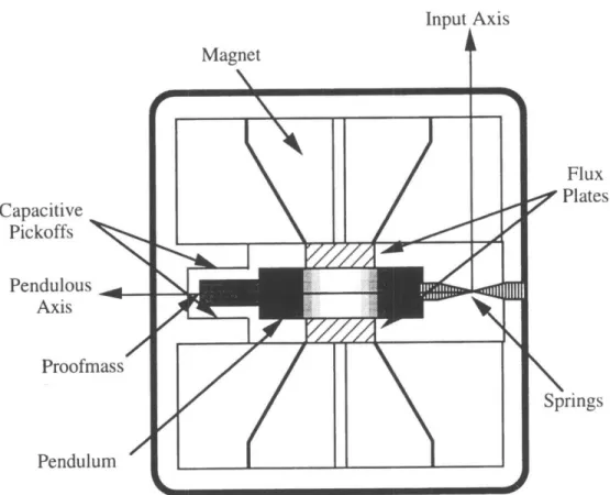
Another feature that keeps the accelerometer characteristics linear is a constant magnetic field through the center of the coil. Figure 1.2 shows how the pendulum structure is situated within the magnets, flux plates, and capacitive bridge pickoff. The magnetic field is generated using two axially-symmetric magnets separated by a pair of flux plates [3]. The flux plates are placed in the center of the coil carrying the torquing current. The flux plates maintain a constant, radial, high-density magnetic field through the coil by concentrating and redirecting the magnetic flux lines from the two magnets.

The deflection of the pendulum is measured through a capacitive bridge pickoff [3]. In its undeflected or null position, the pendulum lies centered between two plates of a capacitor. This effectively creates two equal capacitors. When the pendulum is deflected, the balance between the capacitors is disrupted and a phase shift results in the

Input Axis Flux Capacitive Plates Pickoffs Pendulous , . Axis Proofmass Springs Pendulum

Figure 1.2: Simplified Pendulous Accelerometer Cross Section

a.c. signal passing through the bridge circuit. The shifted signal is then demodulated and used in the servo loop to generate the restoring current. The pendulum is forced back to its null position and the restoring current is measured.

1.2.3 Errors in Accelerometers

Although accelerometers are designed for linearity, there are many sources of error that prevent a simple linear relationship between the input acceleration and the restoring current. Some error sources appear in both strapdown systems and gimbaled systems. These errors include biases, scale factors, g-squared terms, misalignments, and higher order terms. Other error sources are dynamic in nature and only appear in strapdown systems. These dynamic error sources include anisonertia terms, output axis coupling terms, and size effects. Still other error sources are introduced when testing or

calibrating the accelerometers. The two error sources due to testing are lever arms to the center of the table and non-incident gimbal axes.

1.2.3.1 Static Errors

Although the accelerometers are built very carefully, they are not perfect. Even if there are no forces acting on the body, the accelerometers may still show an output, called a bias. This output exists because the proofmass may actually have a null position that is offset from the assumed null position. If the bias is known it may be subtracted from the output to arrive at the true acceleration.

Another error source is the scale factor of the accelerometer. The scale factor is the proportionality constant between the measured acceleration and the actual acceleration. This proportionality constant may not be known precisely. Also, the scale factor for a positive acceleration may be different than the scale factor for a negative acceleration. The difference between the two scale factors arises from the torque rebalance loop in the accelerometer. Therefore, there are generally two separate scale factors for a given accelerometer.

G-squared terms are one more source of error for both strapdown and gimbaled systems. "G-squared" means the terms depend on either the square of a single acceleration, or the product of two orthogonal accelerations. The squared acceleration terms are a result of nonlinearities in the accelerometer. These errors are usually observed when the acceleration along the input axis is very large. The large input accelerations will cause the pendulum to deflect significantly, producing nonlinear characteristics. G-cubed terms, which depend on the cube of the input acceleration, are also a result of nonlinearities in the accelerometer.

The g-squared error terms are also sensitive to two orthogonal accelerations. For example, suppose the body is being accelerated along the pendulous axis of one of the accelerometers. Since the acceleration is orthogonal to the input axis, there will be no output for that particular accelerometer. However, the pendulum itself will be slightly

stretched and the center of mass of the pendulum will move along the pendulous axis. The relationship between an acceleration along the input axis and the restoring current will now be different for this accelerometer, because the moment arm of the pendulum has

changed.

Another contributing factor to the g-squared error is that the pendulum never actually makes it back to the null position. In order to measure an acceleration at all, the pendulum must deflect slightly. Ideally, the pendulum is restored to its null position. This would be true if there were an infinite loop gain. Since the gain is finite, there will always be a null offset that is a function of the input acceleration. This creates a moment arm upon which an acceleration along the pendulous axis may act, causing an error in the measurement. This error mechanism is shown in Figure 1.3. There are other g-squared terms as well. Some of these can be described from a mechanical standpoint, while others are measured experimentally.

Input Axis

Pendulous Axis

Figure 1.3: Null Offset Error Mechanism

Misalignments between the accelerometer axes and the body axes will also result in errors in both strapdown and gimbaled systems. If the three accelerometers are perfectly aligned with the body axes, then the accelerometer outputs will represent the accelerations along each of the body axes. However, if the accelerometer input axes are

misaligned, then the accelerometer outputs will be combinations of the accelerations along the body axes. If these small misalignment angles are known, then the accelerations along the body axes may be computed from the accelerometer outputs.

1.2.3.2 Angular Motion Errors

Some of the error sources in accelerometers only appear in strapdown configurations. These errors are a result of body angular rates and angular accelerations. In strapdown systems, the accelerometers experience the same angular motion as the body because they are rigidly attached to the body. This angular motion produces errors in the indicated accelerations. The error terms due to this angular motion are anisonertia terms, output axis coupling terms, and size effect terms.

When the INS unit is spun about some axis with a constant angular velocity, there will be some indicated linear acceleration. This indicated acceleration will be due, in part, to the centripetal acceleration of the center of mass, which will typically have some component along the input axis of one or more of the accelerometers. For certain spin axes, the resultant acceleration output will be minimized. The point on the pendulous axis through which these minimum acceleration axes pass is called the center of spin. The distance from this point to the hinge depends on the difference between two of the moments of inertia of the pendulum. Hence, these error terms are called anisonertia terms.

Similarly, when the INS unit is subjected to an angular acceleration, there will be an output that depends on the location and the orientation of the axis of angular acceleration. Once again, there is a point along the pendulous axis through which any axis of angular acceleration will result in a minimum output acceleration. This point is defined as the center of angular acceleration. When the system experiences an angular acceleration about this point, the torque developed at the hinge enables the pendulum to keep up with the angular acceleration of the encasement. Hence, no error torques are developed and there will be no indicated acceleration. Since this error depends on the

acceleration about the output axis, the corresponding error terms are called output axis coupling terms.

Size effects are another error source for strapdown systems. These terms refer to the distances between the three accelerometers, their orientations to one another, and the small internal distances within the accelerometers. In a gimbaled system, these distances are unimportant because the rotation of the body does not affect the output of the accelerometers. However, in a strapdown system the accelerometers are subjected to angular velocities and angular accelerations. These angular motions will translate into error torques and indicated accelerations that are functions of the size effect terms. Therefore, the distances between the accelerometers and both the spin and angular acceleration axes are significant error sources.

1.2.3.3 Testing Errors

A group of accelerometers may be calibrated by placing them on a three-axis test table and rotating the body about all three axes. Calibrating the accelerometers will accurately determine all the error terms. However, still more error terms are introduced by using a test table. The test table provides two major error sources: lever arms to the center of the table and non-incident gimbal axes.

The lever arm terms dictate how the table's angular rates and accelerations affect the output of the accelerometers. The errors due to the table's angular motion will be greater for accelerometers that are farther away from the center of the table. These distances must be determined accurately in order to calibrate the other error terms of the accelerometer.

Ideally, all three axes of the test table intersect at one point. This provides a center of rotation that is the same for all of the table axes. However, the gimbal axes do not intersect at one point. The nominal calibration test consists of mounting the INS on the inner gimbal such that the reference point in the INS is at the center of the test table. If the axes all intersected at one point, then the INS reference point would experience no

motion, and the position outputs of the navigator could be compared to a nominal zero position. However, if all the gimbals are being rotated, every point in the inner gimbal frame will experience some type of motion due to the displacements between the gimbal axes. Therefore, the navigator position must be compared to the estimated displacement of the navigation reference point.

1.2.4 Error Terms Calibrated in This Thesis

This thesis calibrates the dynamic error terms of a group of strapdown accelerometers. It is assumed that the accelerometer's static error terms are already calibrated. The static terms include the biases, scale factors, and the g-squared terms. These are the terms present in both gimbaled and strapdown systems. Static error sources may be calibrated without using a dynamic test table. If the static error terms are already calibrated, then the navigator can compensate for these errors. The only remaining errors will be depend solely on angular motion.

In addition to calibrating the dynamic error terms, the thesis must also address the errors introduced during testing. These errors include the lever arms to the axes of rotation as well as the small displacements between the gimbal axes. The displacements between the gimbal axes must be measured accurately because the accelerometers will be used on a body that experiences very high angular rates and accelerations. Therefore, the test table will be spun at high rates with correspondingly high angular accelerations. These large angular rates and accelerations will produce noticeable errors even if the

displacements between the gimbal axes are very small.

1.3 Previous Work

Calibration of inertial navigation systems has been a heavily studied area. Error models for both gyros and accelerometers are developed in many references [1,4,5]. The application of optimal estimation to the calibration problem, using Kalman filtering and optimal smoothing techniques, has been investigated [6,7,8]. Both in-flight calibration

and laboratory testing have been addressed [9]. However, most of these calibration studies focus on the effects of accelerometer biases and scale factors, while either ignoring the angular motion errors or lumping them into a general error term. It is true that the scale factors and biases are the dominant error terms in most applications. However, the errors induced by angular motion become significant when the vehicle experiences very large angular accelerations and velocities.

Some recent work has been done on calibrating the angular motion errors [10,11]. Test table trajectories were developed in order to observe some or all of these error terms. However, these trajectories were either not optimal or only designed to calibrate one of the error terms.

The goal of this thesis was to develop a trajectory that allowed calibration of all the error terms introduced due to angular motion. The trajectories developed in the thesis were designed to reduce the uncertainties in the error terms compared to a previous trajectory. The effects of changing various trajectory characteristics were also investigated. The tradeoff between observability and sensitivity of the error terms was performed by designing trajectories that emphasized either the observabilities or the sensitivities and analyzing the effects on the uncertainties of the error terms. The trajectories that produced the lowest uncertainties were identified. By applying the testing techniques described in these trajectories, the effects of angular motion on an INS may be compensated out with a greater degree of accuracy. The end result will be more accurate navigation in the presence of large angular rates and accelerations.

Chapter 2

Analytic Development

2.1 Accelerometer Error Model

An accurate error model must be derived in order to calibrate the set of accelerometers. This error model will be used in the simulation to relate the accelerometer error coefficients to the errors in navigation. Once the accelerometer error coefficients are accurately estimated, the effects of angular motion on the accelerometer outputs can be compensated out, providing the true linear accelerations experienced by the vehicle.

2.1.1 Assumptions on Previously Calibrated Quantities

Static calibration tests will already have been completed before the dynamic testing of the accelerometers is performed. Optimum test table positions for calibration of the static error terms are described in [12]. These tests calibrate the accelerometer error terms that are independent of angular motion. These error terms include the positive and negative scale factors, g-sensitive terms, g2-sensitive terms, and the accelerometer biases. These are the error terms that produce errors in the indicated accelerations due to linear accelerations of the vehicle. The uncertainties of these initially calibrated values are also given in [12].

Since the error terms associated with linear accelerations are assumed to be calibrated, the only errors in the navigator will be due to the accelerations developed as a result of angular motion.

2.1.2 Angular Effects on Accelerometer Output

The dynamic error terms relate angular motion of the vehicle to errors in the indicated accelerations. In order to determine the errors in the navigation solution, an equation that relates angular velocity and angular acceleration to errors in indicated acceleration must be developed. The following development of the error acceleration equations follows the derivation contained in [3].

2.1.2.1 Angular Velocity Sensitivity

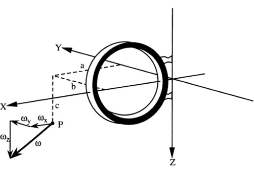
Figure 2.1: Angular Velocity Acting on Accelerometer

In this section we determine the effects of angular spin on the output of the accelerometers. Referring to Figure 2.1 we define a point P through which the spin axis passes. The direction of the spin axis given in terms of the pendulum coordinate frame is

wo= i + 0,j+owk, where i,

j,

We need an equation that relates angular velocity to the error torque developed about the accelerometer's output axis. This equation can be derived by summing the torques developed, due to angular rotation, of each mass element of the pendulum. Some preliminary definitions are needed:

r, = xi+ Yj+ Zk

r,= (X, -a)i +(Y, - b)j+ (Zi - c)k

where

ri = position vector from the accelerometer frame origin to the ith mass element

r = position vector from point P to the ith mass element

w = angular velocity vector in the accelerometer frame

The force on the ith mass element due to the centripetal acceleration produced by the angular velocity vector w is:

f i = mi ) x (( X r')

where mi is the mass of the ith element. This can also be written as: f, = m,[g(, r") - r (o -o))]

The torque about the origin of the accelerometer frame is then:

", = r xf, = m,[r, x co(qo-r)-r, x r"'(, t)] (2.1) where we note that:

CO -O) = (02 = 2 2 2

_ lr' = (Xi -a)ox +( Yi - b)(, +(Z, - c)(o_z

ri

i j k +[Y, (Zi -c)- Z,(Y -b)]i

r, r,'= X, Z, = -[x,(Z -c)- Z,(X, -a)]j X,-a Y,-b Z,-c +[X(Y -b)-Y (X, - a)]k

The error in indicated acceleration will be due to the torque developed about the output axis of the accelerometer as a result of the angular velocity. Therefore, we are only interested in the torque about the Z-axis. Substituting the above relations into equation (2.1), we have:

Tz = m, {[(X, _{- a)o, +(Y, -b)w, +(Z, -c)(WO](XOW - Yw x)}

- W2(aY - bX)} (2.2)

We sum over all the mass elements to determine the total resultant torque. When summing over all the mass elements we note that:

I mi (X + )= lyy

I m, (Yi2 + Z2) IXX

I, = m,X,Yr, , I.z = mYZi , I, = Y m,Z,X, Mlo = mX

where

Ixx, Iyy = pendulum moments of inertia about the X and Y axes

Iij = product of inertia with respect to the i and j axes M = total mass of the pendulum

10 = distance along the X axis between the hinge and the center of mass of the

pendulum

Performing the indicated substitutions, we arrive at the general formula for the torque about the Z-axis:

Tz = (Iy, - Ix -aMlo + bm,Y,)(ox, +(Ixz - cMlo) (yo.

+(c mlY, - Ivz)( OxO z + lxy( 2 - 02)+ a(xmiY, (2.3)

The pendulum is designed to be symmetrical about the origin of the accelerometer frame along both the input and output axes. Therefore, the products of inertia and Im, Y, are very small. Eliminating these terms we arrive at:

"r = (I, - xx - aMlo)wxo, - cMlowoyo - bMlow + bMloo 2

or

Tz = (Iy, - Ix - aMlo0)xw - cMloawoz + bMlo(w2 + 0)

Writing this equation in terms of the accelerometer's pendulous, input, and output axes we have:

,, = (I,i - Ipp - aMlo)tcoip - cMlowoo,, +bMlo (w +

,

This is the expression for the error torque developed about the pendulum's output axis due to the angular velocity vector (o. This equation is valid for all three accelerometers, as long as the orientation of the pendulous, input, and output axes are the same as those defined in Figure 2.1.

If the spin axis is defined to go through the pendulous axis (b=O, c=O), then the only term left in equation (2.4) will depend on the difference of two moments of inertia and the angular velocities about the input and pendulous axes. This error term is then referred to as an anisonertia term. In order to minimize the error torque, the value for a can be chosen so that,

Ii -I

a = I = X,

Mo

This point is called the center of spin, because no error torques are developed if the spin axis passes through this point on the pendulous axis.

2.1.2.2 Angular Acceleration Sensitivity

The pendulum will also experience a torque about the output axis when an angular acceleration is applied. This angular acceleration can be represented in the accelerometer frame as:

d

--dto = = i + oyj + ozk

-The force on the ith particle due to the angular acceleration will act in the tangential direction to the angular acceleration and is given by:

f = m,, xr

Therefore, the torque about the origin is:

", = r, x f, = mir, x (a x r')

or

T, = m,[a(ri -r') - r'(a -r,)] (2.5) where

r, .r, = X,(X,-a)+ Y,(Y,-b)+ Z,(Z, -c)

a -ri = axX, + aY, + a,Z_,

Once again, we are only interested in the torque about the Z-axis. Therefore, we substitute the above expressions into equation (2.5) and get:

Z, = m,[(X2 -aX, + Y,2 -bY, + Z -cZ)Oaz -(axXi + avY, + cxzZ,)(Zi -c)] (2.6)

Summing over all the mass elements and using the previous definitions for the moments and products of inertia we obtain:

7 = (Iz - aMlo - bm, Y, )oa - (Ixz - cMl0o)x - ( vz - cm, Y, )

a,

Eliminating the products of inertia and the Xm, Y, terms and expressing the result in terms of the accelerometer's pendulous, input, and output axes we have:

T,, = (I,,,, - aMlo)a, + cMlo , (2.7)

This is the expression for the error torque about the pendulum's output axis that results from the angular acceleration vector a.

If the spin axis is defined to pass through the pendulous axis (b=O, c=O) in this case, then the error torque will depend only on the output axis moment of inertia and the angular acceleration about the output axis. This error term is referred to as an output axis coupling term. Once again, an appropriate value for a can be chosen to minimize the error torque. Specifically, for the case of angular acceleration, the minimizing value for a is

I

a = . - Xa

This point is referred to as the center of angular acceleration or the effective center of mass, because no error torques are experienced if the angular acceleration axis passes through this point on the pendulous axis.

2.1.2.3 Total Sensitivity to Angular Motion in Accelerometer Frame

Using the definitions for the centers of spin and angular acceleration, the total error torque developed due to angular motion in the accelerometer frame can be written as:

,.tort, = Mlo[(X, - a)Wiop - ci ,, + b( o + 0, ) + (X - a),, + ca]

Since the error in indicated acceleration due to the error torque is given by:

"o,total

aerror - " otal

P

where P is the pendulosity of the pendulum and is defined as M1o, then the acceleration error is:

aerr,,r =(X - a)co, O)-COio)O +b(~ ) + (X - a)a,, + ca, (2.8) This acceleration error was determined assuming that the pendulum frame was identical to the frame in which the spin axis was defined. However, the angular velocity will be known in the accelerometer case frame rather than the pendulum frame. Since the pendulum may not be aligned with the accelerometer case's pendulous axis, additional errors will be generated. These errors are due to the resultant torque components along the pendulum's output axis. The orientation of the pendulum's axes (p', i', o') to the accelerometer case axes (p, i, o) is shown in Figure 2.2, where Pp, Bi, and

Po

VP = C v

= [I - X(f' )]v'

where X(P) is the cross product matrix of the misalignment angles. The additional error in indicated acceleration is a function of the resultant torque component about the pendulum's output axis [3,14]:

Saerror = (AXa - 1,cp)a, + [f,,c - , (Xa - a)l]a, - ,ba,,

+( ,c - f,, X,,,)(0 + [p,,c + f,,(X, - a)]0,2 - floaw, +flobo ,o, + [,,c + p(X,, - a)k],wp(, - (f,b - fl,,,)oo

0o

Misalignment of Pendulum Axes About Case Axes

Combining the errors in (2.8) and (2.9), an equation for the total acceleration error that takes angular velocity, angular acceleration, and misalignments into account can be written:

8aloua = (c + iXa _{- ,Oc)a,, + [/,,c - ,,(Xa - a)]a, + (X, - a - fb)a,,}

+(b +,,c - ,,o,,) + [P,,c + P,,(X,O - a)] , + (b - #,,a) ( (2.10)

+(X,O - a + fob)o,,po, + [0,,c +

fl,,(X,,

(2.9)

o p

2.1.3 Reduction of Parameters into Angular Dependent Coefficients

The dynamic error terms are represented in this thesis by nine coefficients for each

of the three accelerometers. The nine error coefficients are combinations of error

parameters arising from lever arm effects, size effects, anisonertia effects and output axis coupling effects. The general equation for acceleration error in a given accelerometer can

be written as:

ai = Cil ax + C2, y + Ci3a z

+c 4 )2 2+ c, 6 1 2 (2.11)

+Ci7 )x + Ci8 x z + C9 0y o z

where

Sai = acceleration error in the ith (X, Y, or Z) accelerometer cij = jth error coefficient for the ith (X, Y, or Z) accelerometer

(x, 0y, xz = angular acceleration along the accelerometer case X, Y, and Z axes

Ox,

Wy,

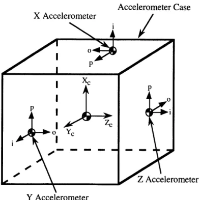
In order to write the acceleration error equations for all three accelerometers, the orientation of the accelerometers to the case must be defined. The orientation shown in Figure 2.3 [14] was used for the simulation, where p, i, and o denote the pendulous, input and output axes for each of the accelerometers. This orientation was based on the assumption that the maximum angular velocities and angular accelerations will be along the X-axis of the case. In order to minimize the effects of the output axis coupling terms, none of the output axes of the accelerometers were placed along the X-axis [15]. Table 2.1 summarizes the relations between the case axes and the axes for the X, Y, and Z accelerometers. The coefficients for each accelerometer, as represented in (2.11) were determined using equation (2.10) and Table 2.1. Table 2.2 lists the combinations of accelerometer parameters that make up the error coefficients. Note that the lever arm distances a, b, and c were replaced with Rij terms, where the "i" subscript refers to the

Accelerometer Case

Z Accelerometer Y Accelerometer

Figure 2.3: Orientation of Individual Accelerometer Axes to Case Axes

accelerometer (X, Y, Z) and the "j" subscript refers to the appropriate case axis (X, Y, Z).

The combination of accelerometer parameters into error coefficients was done for two reasons. First, many of the error terms are not separable. For example, referring to equation (2.10), an angular acceleration about the case's output axis (co) would produce an indicated acceleration because of an output axis coupling term (Xa-a) and a

Table 2.1: Accelerometer Axes to Accelerometer Case Axes Relations

Accelerometer Individual Axes Accelerometers X Y Z Pendulous +Yc +Xc +Xc Input +Xc +Yc +__ Output -Zc +Zc -Yc

Table 2.2a: X-Accelerometer Error Coefficients cl _ x 3xzRxz-oxyXax+3xyRxy C12 Y -Rxz+pxxXax+ 3xyRxz C13 az -Xax+Rxy-pxzRxx C14 1 x2 -PxyRxz-pxzXox+xzRxy C15 YO2 Rxx-IxyRxz+PxzXcox c16 (z2 Rxx+pxzRxy c17

Oxoy

0

x

C21 ax Ryz+PyyXay-iyxRyz c22 X V PYzRyz-pyxXay+pyxRyx c23 _ z XOay-Ryx-iyzRyy c24 )x2 Ryy+yxRyz-yzXy c25 _ Y2 _ yxRyz+yzXoy-yzRyx c26 Oz2 Ryy-pyzRyx C27

(OXCOY

oxOz

c29 __y_-Oz -Ryz- vxRyy+yyXoy

misalignment and lever arm term (-Pob). The errors due to these two terms cannot be determined individually, but rather as a combination of their effects.

Table 2.2c: Z-Accelerometer Error Coefficients c31 0x_ -Rzy+PzzXaz+pzxRzy c3 2 , -Xaz+Rzx-3zyRzz c33 0z PzyRzy-I3zxXaz+p3zxRzx c34 Cx 2 Rzz-pzxRzy+pzyXoz c35 Y2 Rzz+pzyRzx c36 0z2 -PzxRzy-]zyX oz+pzyRzx c37 COxWyY -PzyRzy+pzxXoz- pzxRzx c38 0xOz Xoz-Rzx-zyRzz c39 0ycoz -Rzy+PzxRzz-pzzXoz

The second reason the accelerometer parameters were combined into error coefficients is that by grouping the parameters into nine coefficients, the estimation problem becomes a linear filtering problem. The coefficients are actually sensitivities of the acceleration error to the angular accelerations, angular velocities squared, and the products of the angular velocities in the accelerometer case frame. The final result of processing the error acceleration equations using the coefficients will be accurate estimates of the sensitivities of the acceleration error to angular motion. These sensitivities may then be used to compensate out acceleration errors due to vehicular angular motion.

2.2 Simulation Model

This section describes the tools used to perform the simulation. The testing method using a three-gimbal test table is outlined. The equations are presented for the covariance analysis using a Kalman filter. The unique characteristics of the Kalman filter are described in detail.

2.2.1 Test Table

The test table used in the simulation is a three-axis motion simulator. The three orthogonal axes allow control over the dynamic motion of the INS system, which is rigidly mounted inside the innermost gimbal of the table. Figure 2.4 is a picture of a typical three-axis gimbal test table.

Mounting Plate

Pitch

Figure 2.4: Three-Axis Gimbal Test Table

Figure 2.4 shows that the outer, middle, and inner gimbals control deflections about the yaw, pitch, and roll axes, respectively. For the configuration shown, the yaw and roll angles are zero and the pitch angle is 90 degrees.

The control inputs to the test table were individual gimbal angular accelerations. By controlling the gimbal angular accelerations, a wide range of angular motions for the

system inside the test table were developed. The type and limitations of the specific table assumed for this thesis are detailed in Section 3.1.2.

2.2.2 Navigator Position

A static calibration of the INS will already have been performed. This calibration

allows the INS to navigate in the absence of angular motion. Since the test table subjected the INS to angular motions, and no linear motions, the nominal navigator position output was zero. This assumed that the reference point in the INS was at the intersection of all three table gimbal axes. Also, it was assumed that the navigator compensated for the gravity vector effects. However, the angular motion of the INS would produce nonzero outputs in the accelerometers. These outputs would then be integrated in the navigator, yielding a nonzero position. Therefore, the outputs of the navigator were assumed to be the errors due solely to angular motion.

The navigation reference point must lie at the intersection of all three gimbal axes in order for the navigator to have a nominal position output of zero for all possible gimbal motion. However, as mentioned in Section 1.2.3, the gimbal axes of the test table do not intersect at a point. The table manufacturer specifies a small sphere, inside of which the table axes intersect. The gimbal axis displacements will result in motion of the navigation reference point, regardless of where it is placed inside the inner gimbal. To compensate for the effects of the gimbal axis displacements, the position vector from the origin of the local level frame to the origin of the inner gimbal frame must be estimated. The equations that give this position vector as a function of the displacements and the gimbal angles are derived below [16].

2.2.2.1 Gimbal Axis Displacements

The origin of the local level frame and the outer gimbal frame may be defined to be the same point, 00. This point was defined to be the intersection of the outer gimbal axis and the plane of the middle gimbal frame, as shown in Figure 2.5. The outer gimbal coordinate axis og 1 was defined to be perpendicular to the middle gimbal spin axis, and pointing toward the middle gimbal spin axis in the plane of the middle gimbal frame.

Then, the position vector from the origin of the outer gimbal frame to the origin of the middle gimbal frame was constant in outer gimbal coordinates and was given by:

r,, = (PoMI, 0, 0) (2.12)

where POMI is the displacement between the outer and middle gimbal axes. The subscript "OM" denotes the position vector from the outer gimbal origin to the middle gimbal origin, and the superscript "og" denotes the vector is expressed in outer gimbal frame coordinates.

og3, outer gimbal spin axis

mg3

em

middle gimbal spin axis

ogl

Figure 2.5: Middle Gimbal Origin in Outer Gimbal Frame

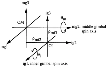
Similarly, the origin of the inner gimbal frame was displaced from the origin of the middle gimbal frame, as shown in Figure 2.6. The position vector from the middle gimbal origin to the inner gimbal origin was constant in middle gimbal coordinates and was given by:

rM, = (0, PMI2 PM13) (2.13)

mg3

mgl

middle gimbal spin axis

Figure 2.6: Inner Gimbal Origin in Middle Gimbal Frame

gimbal origin along the middle gimbal mg2 and mg3 axes, respectively. As before, the subscript "MI" means the vector is from the middle gimbal origin to the inner gimbal origin, and the superscript "mg" means the vector is expressed in middle gimbal frame coordinates.

The position vector from the origin of the local level frame to the origin of the inner gimbal frame was then expressed in the middle gimbal frame as:

mg mg + rmg Cmg"r" + rm og OM MI cos ,O 0 -= 0 1 sin Om 0 c

[

1

O

This vector was expressed in inner gimbal coordinates by multiplying by the middle to inner gimbal frame transformation matrix, C'~: