Final report: tests to assess the effect of model construction on resistance

(1)

Publisher’s version / Version de l'éditeur:

Laboratory Memorandum, 2015-10

READ THESE TERMS AND CONDITIONS CAREFULLY BEFORE USING THIS WEBSITE. https://nrc-publications.canada.ca/eng/copyright

Vous avez des questions? Nous pouvons vous aider. Pour communiquer directement avec un auteur, consultez la

première page de la revue dans laquelle son article a été publié afin de trouver ses coordonnées. Si vous n’arrivez pas à les repérer, communiquez avec nous à PublicationsArchive-ArchivesPublications@nrc-cnrc.gc.ca.

Questions? Contact the NRC Publications Archive team at

PublicationsArchive-ArchivesPublications@nrc-cnrc.gc.ca. If you wish to email the authors directly, please see the first page of the publication for their contact information.

For the publisher’s version, please access the DOI link below./ Pour consulter la version de l’éditeur, utilisez le lien DOI ci-dessous.

https://doi.org/10.4224/21277547

Access and use of this website and the material on it are subject to the Terms and Conditions set forth at

Final report: tests to assess the effect of model construction on

resistance

Pallard, Rob

https://publications-cnrc.canada.ca/fra/droits

L’accès à ce site Web et l’utilisation de son contenu sont assujettis aux conditions présentées dans le site

LISEZ CES CONDITIONS ATTENTIVEMENT AVANT D’UTILISER CE SITE WEB.

NRC Publications Record / Notice d'Archives des publications de CNRC:

https://nrc-publications.canada.ca/eng/view/object/?id=79443479-bc78-4dd6-ac89-f2768cf3e40f https://publications-cnrc.canada.ca/fra/voir/objet/?id=79443479-bc78-4dd6-ac89-f2768cf3e40f

(2)

OCRE-LM-2015-002

FINAL REPORT - TESTS TO ASSESS THE EFFECT OF MODEL CONSTRUCTION ON RESISTANCE

Laboratory Memorandum - Unclassified OCRE-LM-2015-002

V1.0

Rob Pallard

St. John’s, NL

October 2015

(3)

(4)

(5)

Ocean, Coastal and River Génie océanique, côtier et fluvial Engineering

FINAL REPORT - TESTS TO ASSESS THE EFFECT OF MODEL CONSTRUCTION ON RESISTANCE

Laboratory Memorandum

UNCLASSIFIED

LM-2015-002

V1.0

Rob Pallard

October 2015

(6)

(7)

Abstract or Executive Summary

This report describes the bare hull resistance experiments carried out on 5 m models of a PANAMAX bulk carrier in April and May of 2015 to assess the effects of proposed changes in model construction techniques on experimental results. Four model options were assessed during this session.

The test results for these four options are compared to the large model originally tested in April 2013 and a repeat test of the large model done as part of this test session. Repeatability tests were done at multiple speeds to estimate the typical uncertainty of a resistance test done in this laboratory.

(8)

(9)

Abstract or Executive Summary ... i

Table of Contents ... iii

Table of Figures ... v

Table of Tables ... vi

1 INTRODUCTION ... 1

2 BACKGROUND ... 1

3 DESCRIPTION OF THE NRCSJS TOWING TANK ... 2

4 DESCRIPTION OF PHYSICAL MODELS ... 2

5 DESCRIPTION OF INSTRUMENTATION AND DATA ACQUISITION

SYSTEM ... 3

5.1 Standard Resistance Test Instrumentation ... 3

5.2 Data Acquisition System ... 5

6 DESCRIPTION OF THE EXPERIMENTAL SET UP ... 5

7 DESCRIPTION OF THE TEST PROGRAM ... 6

7.1 Bare Hull Resistance ... 6

8 ONLINE DATA ANALYSIS PROCEDURE ... 6

8.1 Bare Hull Resistance ... 6

9 OFFLINE DATA ANALYSIS ... 7

10 QUALITY ASSURANCE ... 7

11 DISCUSSION ... 8

11.1 Resistance Curve ... 8

11.2 Repeatability Sets ... 9

11.3 Sinkage and Trim ... 10

11.4 Uncertainty Analysis ... 11

12 RECOMMENDATIONS ... 12

13 ACKNOWLEDGEMENTS ... 13

14 REFERENCES ... 13

TABLES ... 15

FIGURES ... 27

Appendix A – Model Hydrostatics and Floatation QA ... A-1

Appendix B – Calibrations ... B-1

Appendix C – Run Log ... C-1

Appendix D – Results of Resistance Experiment ... D-1

Appendix E – Model Resistance Coefficients ... E-1

(10)

Appendix F – Sinkage and Trim ... F-1

Appendix G – Balance Verification Tests ... G-1

(11)

Table of Figures

Figure 1: OCRE 931 as installed in the Towing Tank ... 28

Figure 2: Turbulence Stimulation for OCRE 930/931 ... 29

Figure 3: Resistance at 15 deg C in Fresh Water – prediction at size of large model

(OCRE916) April-May 2015 ... 30

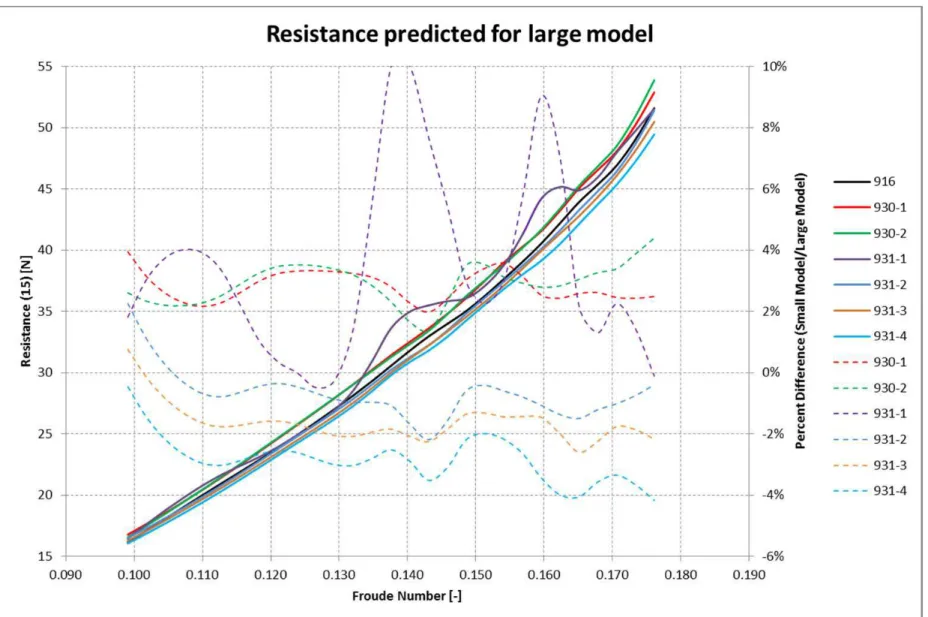
Figure 4 : Resistance at 15 deg C in Fresh Water – prediction at size of large model

(OCRE916) January 2015 ... 31

Figure 5: Repeatability at Fr=0.10 ... 32

Figure 6: Repeatability at Fr=0.13 ... 33

Figure 7: Repeatability at Fr=0.17 ... 34

(12)

Table of Tables

Table 1: List of Signals ... 16

Table 2: Test Plan – Small Model ... 17

Table 3: Test Plan – Large Model ... 17

Table 4: Re-analysis of April 2013 OCRE916 dataset using deltaV corrector ... 18

Table 5: Standard Uncertainty of Calibration for Small Model ... 19

Table 6: Standard Uncertainty of Calibration for Large Model ... 20

Table 7: Summary of Prediction of Large Model Resistance for April/May session ... 21

Table 8: Summary of Prediction of Large Model Resistance for January session ... 23

Table 9: Summary of Repeatability Tests –April/May Session ... 24

Table 10: Summary of Repeatability Tests – January Session ... 25

Table 11: Summary of Repeatability Tests – Sinkage and Trim ... 26

Table A1: Summary Hydrostatics ... A-2

Table A2: Float QA – OCRE930B – Day 1 ... A-3

Table A3: Float QA – OCRE930B – Day 2 ... A-4

Table A4: Float QA – OCRE930B – Day 3 ... A-5

Table A5: Float QA – OCRE930B – Day 4 ... A-6

Table A6: Float QA – OCRE931 – Day 5 ... A-7

Table A7: Float QA – OCRE931 – Day 6 ... A-8

Table A8: Float QA – OCRE933 – Day 1 ... A-9

Table A9: Float QA – OCRE933 – Day 2 ... A-10

Table A10: Float QA – OCRE933 – Day 3 ... A-11

Table A11: Float QA – OCRE933 – Day 4 ... A-12

Table A12: Float QA – OCRE916 – Day 1 ... A-13

Table E1: Model Resistance Coefficients - TRUFOAM – April 21 ... E-2

Table E2: Model Resistance Coefficients – TRUFOAM – April 22 ... E-4

Table E3: Model Resistance Coefficients - Standard – April 23 ... E-6

Table E4: Model Resistance Coefficients – Standard – April 24 ... E-8

Table E5: Model Resistance Coefficients – Standard – April 27 (set 1) ... E-10

Table E6: Model Resistance Coefficients - Standard – April 27 (set 2) ... E-12

Table E7: Model Resistance Coefficients – Wooden Model – May 5 ... E-14

Table E8: Model Resistance Coefficients – Wooden Model – May 6 ... E-16

Table E9: Model Resistance Coefficients – Wooden Model – May 7 ... E-18

Table E10: Model Resistance Coefficients – Wooden Model – May 12 ... E-20

Table E11: Model Resistance Coefficients – Large Standard – May 15 ... E-22

Table F1: Sinkage and Trim – TRUFOAM – April 21 ... F-2

Table F2: Sinkage and Trim – TRUFOAM – April 22 ... F-4

Table F3: Sinkage and Trim - Standard – April 23 ... F-6

Table F4: Sinkage and Trim – Standard – April 24 ... F-8

Table F5: Sinkage and Trim – Standard – April 27 (set1) ... F-10

Table F6: Sinkage and Trim – Standard – April 27 (set 2) ... F-12

Table F7: Sinkage and Trim – Wooden Model – May 5 ... F-14

Table F8: Sinkage and Trim – Wooden Model – May 6 ... F-16

Table F9: Sinkage and Trim – Wooden Model – May 7 ... F-18

Table F10: Sinkage and Trim – Wooden Model – May 12 ... F-20

(13)

Table F11: Sinkage and Trim – Large Standard –May 15 ... F-22

Table G1: Summary of Balance Verification Tests – Small Model ... G-2

Table G2: Summary of Balance Verification Tests – Large Model ... G-3

(14)

(15)

1 INTRODUCTION

This report describes experiments carried out on four 1:45 scale models of a PANAMAX bulk

carrier, designated OCRE930-933 in the National Research Council St. John’s (NRCSJS)

Towing Tank in April and May of 2015. Tests with this bulk carrier were originally done at a

scale of 1:31.45 using model OCRE916. The results obtained with model 916, reported in

TR-2013-024 (Reference 1), form the basis for the comparison of the test results. In addition, the

resistance curve for model 916 was repeated using the test instrumentation developed for this

series of tests.

This document includes background information on the project, a description of the

instrumentation, facility used, test program, data analysis procedure and discussion of the results.

It describes the bare hull resistance and repeatability experiments conducted in the Towing Tank

between April 21 and May 13, 2015.

2 BACKGROUND

Over the years, a recurring comment from clients is that our model prices seem high, particularly

when they are compared with the prices charged at other facilities. For example, during

discussions with Garry Cooke and CSL over the cost of the test program for the revisions to the

CSL Metis, it was clear that the major stumbling block was the cost of the model. We were

informed that NRC was competitive with other facilities with respect to experimental testing,

analysis and reporting costs but our model cost was approximately double that of a European

tank.

This prompted NRC-DFS to look at options for model construction that might reduce model

cost. New procedures could potentially make it easier to do some of the typical modifications to

ship models that arise based on the results of model tests. Examples of these modifications

include bilge keel alignment, stabilizer fins and cutaways in way of thruster openings. The

present model construction technique requires that potential locations for these appendages be

locally strengthened prior to final determination of the best location and has a fairly high

up-front design cost. Details of the planned construction procedures and estimates of their relative

costs can be found in Reference 2.

Originally, it was proposed that the optional model construction techniques would be applied to

models of the same scale as OCRE916. The cost of these relatively large models prompted the

idea of using smaller models to assess the construction techniques. Four meter long models were

proposed but the estimated resistance of these models at the median speed of the test program

was about 13 N and a compromise was reached that would have 5 m long geosims built with an

estimated resistance of about 24 N.

For this test, a new piece of resistance test instrumentation was introduced. There was concern

after the January test session that the loads measured during this test were too low to be

adequately discretized by the Kempf and Remmers R35-I balance which has a nominal range of

0-200 N. Maximum resistance with these 5 m long models was less than 25 N or 12.5% of range,

(16)

with most test results between 6 and 17 N or 1.5 - 8.5% of range. This prompted the design and

fabrication of a scalable resistance dynamometer using the measurement principles of the R-35-I

balance but permitting the use of load cells from 10 to 150 lbs (45 to 670 N) that would be better

suited for the estimated load range of a test. For this test, the 10-lb load cell was used. The

balance commissioning tests are described in Reference 3.

3 DESCRIPTION OF THE NRCSJS TOWING TANK

NRCSJS Towing Tank has dimensions of 200 m by 12 m by 7 m. The 85 t tow carriage, capable

of speeds up to 10 m/s, is used to accommodate models for a wide range of test types carried out

in calm water and waves. A 4,000 kg lift capacity moveable overhead crane is available over

half of the tank length.

At the west end of the tank is a dual flap hydraulic wave board capable of generating regular

waves up to 1 m. in height and irregular waves with a signification wave height of 0.5 m. Waves

are absorbed by a parabolic corrugated surface beach with transverse slats at the east end of the

tank. Flexible side absorbers deployed over the entire length of the tank absorb the lateral waves

and minimize the time between runs.

4 DESCRIPTION OF PHYSICAL MODELS

The models are 1:45 scale, nominally 5 m long, representations of a PANAMAX bulk carrier.

They were fitted with a lateral bow thruster opening but no provision was made for rudder, or

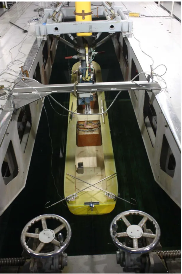
shafting, nor were there any bilge keels fitted to the model. A photo of OCRE931 as installed in

the towing tank is given in Figure 1. Model construction, in general, complied with the

provisions contained in the OCRE model construction standard, GM-1 (Reference 4), except as

noted below.

Model OCRE930 represents the standard OCRE model construction method (option 1) as

described in Reference 1. It uses a plywood box construction at its core. High density

polystyrene foam is laminated to the box to approximate the shape of the ship. High density

epoxy foam, Renshape

TM

, is used locally for areas requiring reinforcement, like the shafting or

bilge keel, or to permit better definition of the shape of the hull in way of a tunnel thruster. The

model surface is milled undersize by about 1-1.5 mm depending on the thickness of the

fibreglass laminate. It is coated with Duratek high build primer left unsanded for the January

phase of the test. For this series of tests, it was sanded, primed and painted with the marine

enamel that is the standard finish used for models since late summer 2014.

Model OCRE931 represents option 3 of the DFS model construction plan. The plug was

laminated using locally produced expanded polystyrene foam, Trufoam

TM

, without a box

structure. The structure of the model consisted simply of two plywood decks. A sprayed on

product was intended to produce the finish surface but proved unsuitable for use with the curved

and vertical surfaces of a ship model. Two layer of 10 oz fibreglass boat cloth were applied to

the plug instead of the “coating” and the model was primed and painted without using the

Duratek product.

(17)

Model OCRE932 represents option 2 of the DFS model construction plan. The plug was

laminated using Renshape™ 5020 high density foam, without a box structure using the

Renshape™ recommended adhesive. The structure of the model consisted simply of two

plywood decks. The laminated model was CNC machined to 0.010” undercut then lightly sanded

and prepped for a final coat of primer and paint on both the external and internal surfaces.

Model OCRE933 represents the wood option of the DFS model construction plan. The plug was

laminated using kiln-dried pine with a nominal thickness of two inches using epoxy resin. The

lumber was jointed and planed to a final thickness of about 1.75 inches. The laminated model

was CNC machined to 0.010” undercut then lightly sanded, coated with polyester resin inside

and out and then, prepped for a final coat of primer and paint on the external surfaces.

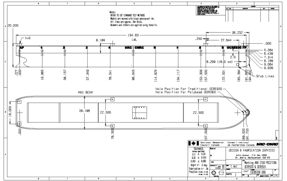
Turbulence stimulation of the hull was placed in a vertical line 16 cm aft of the forward

perpendicular. Turbulence stimulation of the bulb was in a vertical line 5.4 cm forward of the

forward perpendicular. Turbulence stimulation consisted of right cylindrical studs, nominally 3

mm in height and diameter spaced at 25 mm intervals along the girth as shown in Figure 2. An

eye screw was fitted on centerline at deck level at the transom to permit verification of the

resistance measurement system.

In addition to the models described above, the original large scale model, OCRE916, was

re-commissioned, as described in Reference 1, and its load displacement resistance curve repeated.

The models were tested at the following full scale displacement condition: 83548 m

3

volume

displacement, level trim at a draft of 13.5 m full scale. Hydrostatics for the ship and model and

details of the Floatation Quality Assurance are given in Appendix A.

5 DESCRIPTION OF INSTRUMENTATION AND DATA ACQUISITION

SYSTEM

This section describes the instrumentation and calibration methodology used for each parameter

measured on the models. The standard NRCSJS sign convention described in Reference 5 was

followed where:

Trim Angle – positive bow up

Sinkage – positive down

Roll Angle – positive starboard down

Tow Force – positive forward

5.1 Standard Resistance Test Instrumentation

Tow force was measured using a 10-lb Interface SM S-type load cell. Nominal accuracy for this

instrument is shown below.

Nonlinearity - %FS

±0.03

Hysteresis - %FS

±0.02

(18)

Model sinkage and trim was measured using a pair of Celesco PT100 Series cable extension

transducers attached to the model nominally at the fore and aft perpendiculars. Dynamic trim

was measured using a Heidenhain ROD-250 digital encoder mounted to the pitch pivot of the

towing gimbal. Water temperature was periodically measured manually using a hand-held digital

thermometer submerged at the nominal mean draft depth.

Several type of verification pull load cell were used including a Cooper 10 lb load cell, a

waterproofed 50 lb S-type load and finally, a 10 lb Interface SM S-type load cell similar to the

one used to measure tow force in the dynamometer. The Cooper was used because its weight and

range were appropriate for the balance validation but was found to be insufficiently accurate to

validate the balance performance. It was replaced with a waterproofed 50 lb load cell which has

been adequate for balance verification in the past but the pre-load necessary to have the pull line

horizontal was more than half the balance measurement range. In the end, an Interface SM load

cell was supported by a small piece of aluminum angle which eliminated the need for pre-load

during the balance verification tests. This method would not have been suitable if the load cell

was mounted closer to the waterline but proved acceptable for this series of tests.

The load cells (resistance and verification pull) were calibrated by applying a series of static

weights over the desired measuring range. All NRCSJS calibration weights are verified on

precision digital scales. At the beginning of the resistance test, a series of in-line loads were

applied to the model stern pull point and the output from the resistance load cell compared to the

load cell attached to the stern pull point to verify that the acceleration stops in the gimbal were

not attenuating the measured resistance.

The sinkage (heave) displacement sensors were calibrated using a dedicated apparatus whereby

the yoyo potentiometer cable was attached to a flat plate such that the cable could be adjusted in

discrete increments a known distance from the sensor.

The Heidenhain encoder requires no calibration beyond offsetting its output to match the set

condition of the model.

For the repeat test of OCRE916, the SM-10 load cells used in the towing gimbal and the inline

pull were replaced with SM-25 load cells.

Carriage Speed: Carriage speed is calibrated periodically by setting up two proximity switches

on the ice tank rails at a measured distance apart with companion switches on the tow carriage

linked by cable to the carriage data acquisition system. The towing carriage is operated at a

constant speed between the two switches and the time between activating the switches recorded

on the carriage data acquisition system - thus providing an accurate measure of tow carriage

speed. The carriage speed is calibrated over a range of -0.5 to 2.5 m/s

.

The list of signals is presented in Table 1 and the instrumentation calibration information is

given in Appendix B.

(19)

5.2 Data Acquisition System

The GDAC data acquisition application uses the client-server model of computing. Data flows

continuously from one or more data sources (e.g. sensors) to an instance of the server component

of GDAC, where it is time-stamped and held in memory for a period of time. When the memory

allocated becomes full, old data is discarded to make room for new. While data resides in

memory, it is available for extraction by an instance of the client component of GDAC. An

instance of the client component can simultaneously extract data from multiple instances of the

server component. Extracted data is stored in a single DAQ file, which becomes the starting

point for data analysis.

Examples of instances of client components are:



GDAC Acquisition.



GDAC Calibration.



GDAC Digital Meter.

Examples of service components used in this test include:



One that interfaces with an IMC device.



One that interfaces with the Heidenhain Pitch Encoder.

All acquired analog DC signals were low pass filtered at 10 Hz, amplified as required and

digitized at 50 Hz using NRCSJS’s standard data acquisition system and software.

6 DESCRIPTION OF THE EXPERIMENTAL SET UP

The towing tank was configured as follows for these experiments:

Water Depth: The water depth is fixed at nominally 7 m.

Model Towing Arrangement: The model was towed using the medium tow post and gimbal

modified to accept the scalable resistance dynamometer. The model was towed towards the west

end of the Towing Tank. A yaw restraint is fitted forward of the tow post.

Pull Point: The pull point apparatus used to carry out daily verification of resistance was

installed on the outboard edge at the west end of the tow carriage to enable a standard series of

weights could be applied to the gimbal load cell at the beginning and end of every test day during

the resistance tests. The applied load was verified using an in-line load cell.

Wake Suppression Strategy:

Side Beaches, described in Reference 6, were deployed along the length of both the north and

south side of the tank to suppress the model wake generated wave.

(20)

7 DESCRIPTION OF THE TEST PROGRAM

7.1 Bare Hull Resistance

Bare hull resistance experiments were carried out as per the NRCSJS standard resistance

procedure (Reference 7) from 9 to 17 knots full scale (0.692 to 1.304 m/s model scale) with

repeat runs included for data verification. One of the speed sets was repeated ten times to

determine the variability inherent in the measurement system and to develop a better

understanding of the uncertainty of the measurement. As all speeds were low, more than one

speed could be acquired for each run down the tank. Data was acquired for the displacement

condition described in Section 4.0.

Each model, with the exception of the large model, was tested on at least three different days. At

the conclusion of most test days, the model was removed from the tank. Exceptions are noted in

the test log. The resistance and repeatability test plan is given Table 2 for the small models and

in Table 3 for the large model. The Run Log for all tests in the Towing Tank can be found in

Appendix C.

8 ONLINE DATA ANALYSIS PROCEDURE

An analysis of the preliminary data was carried out on the Tow Tank carriage workstation

throughout the test program to verify the integrity of the acquired data. The carriage operator

was responsible for viewing the time series data for all acquired data using the SWEET software

described in Reference 8. In addition, the following data analysis was carried out during the

experiments:

8.1 Bare Hull Resistance

The data were acquired in GDAC format (*.DAQ files) described in References 9 and 10 and

preliminary online analysis done using the SWEET software described in Reference 8 during the

test to verify the integrity of the acquired data. Because of the Cyber Intrusion, it is not possible

to use the OCRE RSP software for online analysis. The resistance online data analysis was

implemented using SWEET and described as follows:

 The basic resistance channels (forward speed, tow force, sinkage AP, sinkage FP and

pitch) were plotted on screen in the time domain. Start and end times (T1, T2) were

interactively selected for the initial tare segment as well as for each steady state segment.

There was more than one steady state segment if more than one forward speed was

acquired during a single run up the tank – a common situation for low forward speeds.

 The following three plots are displayed on the same screen:

o

Trim (degrees) vs. Froude Number

o

Sinkage (mm) vs. Froude Number

o

Resistance (N) vs. Froude Number

 Run Designation, Acquire Time, Start and End Times (T1,T2) and mean values of

Carriage Speed (m/s), Resistance (N), Sinkage LCB (mm) and Trim (degrees) computed

(21)

over each steady state time segment were output in tabular form for all runs completed

for the given model configuration up to the given run.

The raw test results for the resistance curve and the repeatability tests are given in Appendix D.

9 OFFLINE DATA

ANALYSIS

The following data analysis was carried out after completion of the experimental program to

generate the final data products. Because of the Cyber Intrusion, it was not possible to use the

VMS based RSP software to perform the offline analysis. Part of this analysis suite generates the

blockage correction that must be applied to the data. Scott’s blockage correction method

(Reference 11), as implemented in the RSP software, corrects the value of CTM and maintains

speed but does not lend itself to easy implementation within a spreadsheet. Since speeds were

low, the Scott delta V corrector recommended in ITTC procedure 7.5-02-02-01 (Reference 12)

was used to compute blockage correction. All test results were corrected to 15 deg. C in fresh

water.

The original model 916 dataset was re-analyzed using the same blockage corrector to provide

direct comparison. All comparisons are done on the basis of CTM and Resistance corrected to 15

deg C in fresh water. No form factor was applied. The tabulated results of this re-analysis are

given in Table 4.

The Model Resistance Coefficients corrected to 15 deg. C in fresh water are tabulated for each

runs as follows: Froude number (Fr), Reynold’s Number (10

6

Re

M

), Total Resistance Coefficient

(10

-3

CT

M

), and Frictional Resistance Coefficient (10

-3

CF

M

). In addition, the Resistance

corrected to 15 deg. C and the Residuary Resistance Coefficient (10

-3

C

R

) are tabulated and given

in Appendix E. Statistics for the ten repeat runs are included at the bottom of each table.

Sinkage and Trim are tabulated for each runs as follows: Froude number (Fr), non-dimensional

Sinkage at LCB (10

2

Zv/LM), trim (deg) as measured using the Heidenhain encoder and derived

from the heave potentiometers (

θ

V

) and given in Appendix F. Statistics for the ten repeat runs are

included at the bottom of each table.

10 QUALITY

ASSURANCE

The following measures were taken to ensure the integrity of the acquired resistance data:

ONLINE DATA ANALYSIS: The data were analyzed during the test as described in Section

8.1. Any anomalies in the primary resistance channels were identified. Using the technique of

plotting the acquired data against a comparison curve, it was possible to detect and address even

minor problems immediately. If the data from a given run was found to vary from what was

expected by an unacceptable amount, then the run was repeated. If the variance persisted, the

test was halted and an investigation carried out to determine the source of the problem.

DAILY PULLS TO CHECK RESISTANCE LOAD CELL: Every effort was made to verify the

integrity of the load cell used to measure the resistance load as it was acknowledged that this was

(22)

the single most critical acquired parameter. The resistance gimbal was calibrated prior to the test

by applying a series of known static weights to it using the Cussons Technology Horizontal

Static calibration device. It was then installed in the model tow gimbal balance such that it

remains horizontal with respect to the still waterline independent of model attitude. Mechanical

stops were adjusted to prevent inertial carriage acceleration/deceleration induced forces from

damaging the load cell. A series of in-situ longitudinal loads was applied to the stern of the

model using a dedicated drag verification apparatus fitted on the east end of the towing tank

carriage for this purpose. Because the maximum calibration load for these experiments were

about 40 N, the usual approach for measurement of inline load proved inadequate. The checks

done with the 10 lb Cooper load cell and the waterproofed S-type load cell were unsatisfactory

because of catenary effects on the line and the excessive pre-load needed. A bracket was made to

mount the spare SM-10 load cell and support it horizontally relative to the deck of the model.

This reduced the catenary effect to an acceptable level and since model trim during the load cell

verification runs was less than 0.1 degrees, alignment was considered satisfactory. A light line

was connected to the opposite end of this load cell and extended to the drag verification

apparatus, which was aligned with the longitudinal centerline of the model. This line passed

over three low friction sheaves vertically up and over the west end of the carriage deck such that

weights could be applied using a weight pan on the carriage deck. The height of the post was

vertically adjustable to ensure that the applied load was horizontal. The use of an inline load cell

at the model stern, while it adds an extra instrument to the process, mitigates the unknown effects

of friction in the sheaves. In-situ checks were carried out at the start and end of each test day.

The results of these checks for the small and large models are given in Appendix G.

The residual standard deviation was calculated on the basis of correcting the tow force using the

slope and offset to the inline pull load cell. The Standard Uncertainty of Calibration (SEE)

(Reference 13) was calculated using the uncorrected measured tow force and the measured inline

load. This calculation does not account for the uncertainty in the calibration of the inline load

cell. Tables 5 and 6 summarize the Standard Uncertainty of Calibration calculation for Tow

Force and the Inline load cell instruments used for the small and large model, respectively.

11 DISCUSSION

11.1 Resistance Curve

The results for the resistance curves with OCRE931, OCRE930b and OCRE933 were

extrapolated to the size of model OCRE916 and presented as Resistance at 15 deg C in fresh

water in Table 7 and shown in Figure 3. The table and figure also show the results of the repeat

test with the large model, OCRE916 using the new towing gimbal. All of the test results are

compared to the original running of OCRE 916 in April 2013 in terms of a percentage difference

in Table 7 and shown in Figure 3. The mean value and standard deviation of the percentage

difference for speeds between 11 and 15.5 knots, full scale, is shown for each individual

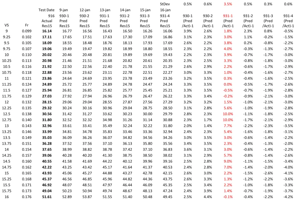
resistance curve at the top of each column. Table 8 and Figure 4 show the same information for

the tests performed in January using the towing gimbal assembled around the Kempf and

Remmers R-35I single component balance.

(23)

No resistance tests were done with OCRE932 as the model had persistent leaks. Three attempts

were made to install this model but as the model was ballasted to its test condition, water

appeared in the model. Two attempts to repair the leaks were made but the location of the leaks

changed with each installation. After the third attempt, the decision was made to abandon tests

with this model.

The bridge model for the two sessions of the tests was OCRE931. This was unfortunate as this

was the model that showed the most variability in the measured resistance in January. This was

mitigated by the repeat test with the large model, originally tested in April 2013, which showed

that the measured resistance repeated within +/- 1% throughout the speed range and between 11

and 15.5 knots, full scale, the mean difference was 0.1%.

For the basic resistance curve, the wooden model (OCRE933) was closest to the large model

while the small standard model (OCRE930b) was furthest from the large model. The April

runnings of the TRUFOAM model were a little closer to the large model than the January

runnings. This is summarized below with information extracted from Tables 7 and 8. Curiously,

the variability of the differences, as characterized by the standard deviation, is larger for the

wooden model than for the other two model construction techniques and the repeat done with the

large model.

April/May Session 930b‐1 930b‐2 931‐6 931‐5 933‐1 933‐3 933‐4 916‐2015 (Pred/Act) ‐1 (Pred/Act) ‐1 (Pred/Act) ‐1 (Pred/Act) ‐1 (Pred/Act) ‐1 (Pred/Act) ‐1 (Pred/Act) ‐1 (Pred/Act) ‐1 Mean* ‐1.8% ‐2.0% ‐1.2% ‐0.7% 0.1% 0.4% 0.6% 0.1% StDev 0.4% 0.5% 0.5% 0.6% 0.9% 0.8% 0.7% 0.5% *Mean and Standard Deviation calculated for speeds from 11 to 15.5 knots January Session 930a‐1 930a‐2 931‐2 931‐3 931‐4 (Pred/Act) ‐1 (Pred/Act) ‐1 (Pred/Act) ‐1 (Pred/Act) ‐1 (Pred/Act) ‐1 Mean* 2.9% 2.9% ‐1.0% ‐1.8% ‐3.0% StDev 0.5% 0.6% 0.5% 0.3% 0.6% *Mean and Standard Deviation calculated for speeds from 11 to 15.5 knots 11.2 Repeatability Sets

As was done in January, ten run repeatability sets were done following the resistance curve of

the day or in some cases as a stand-alone set. The test log, given in Appendix C, contains the

details of the actual test sequence used. The details of the repeatability sets are given in the

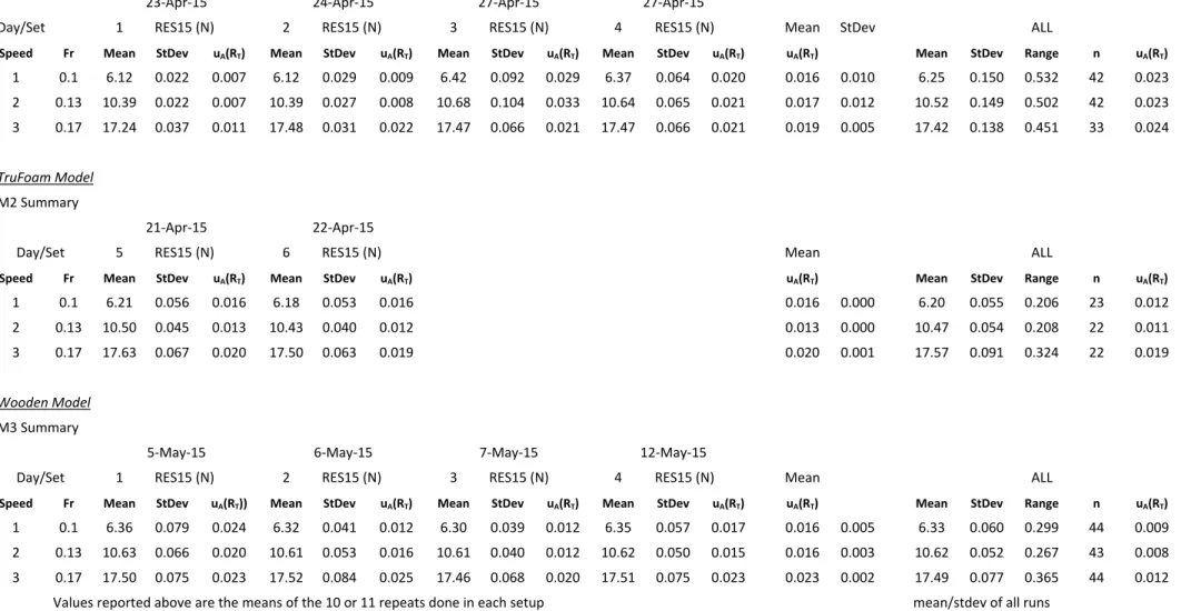
Model Resistance Coefficient Tables (Appendix E) and summarized in Table 9. The summary

table from LM-2005-01, the report on the January tests, is included as Table 10. The variability

in the repeatability sets for the three models for which there were multiple sets of tests is

illustrated in Figures 5 to 7. These figures illustrate the variability by plotting the normal

(24)

distribution of the data derived from the mean and standard deviation of the means of the ten or

eleven repeated runs as Probability Density versus Measured Resistance. The actual measured

data points are superimposed by interpolating the Probability Density curve at the actual

measured value and using that as the abscissa for the point.

The ten repeat runs seem to be a good measure of the uncertainty of the experiment on any given

day. Doing the repeats all together produces the lowest degree of variability and since we were

trying to assess the effects on model construction techniques, this approach has value as it

minimized the effect of run history on the result.

The tables and plots suggest that the wooden model (OCRE933) performs better in terms that

there was less variation from day to day with this construction than with the other two

construction methods.

The other construction methods showed more variability. For the TruFoam model (OCRE931),

this is partly due to it being the bridge model between the two sessions. Two sets from this

session (Day 5 and 6) are compared to two sets from the January session (Day 2 and 3). The

variability at Fr = 0.10 and 0.13 is similar to the wooden model but at Fr = 0.17, the results or

each day group separately with little overlap. This model was less stiff longitudinally than the

other models and displayed more oscillation in the trim and heave time histories. This may be

due to difference in the ballast distribution between sessions and individual installations.

The small standard model (OCRE930) also showed more variability than expected. This is partly

due to the wrong speed being repeated on Day 2 at Fr=0.17 and since time did not permit a

complete repeat, we decided to amend the test sequence to simply do the repeatability sets

without the basic resistance curve. Run sequence has been seen to have an effect on test results in

other tests but usually, as a result, of a large amount of energy being put into the tank or an

inadequate wait time. This was not the case for these tests, but nonetheless the repeatability sets

done without the resistance curve in this session generally displayed higher resistance values.

During the January session, time constraint permitted only the repeatability set to be done on one

day with the unpainted version of this model but the variability described above did not appear.

11.3 Sinkage and Trim

The variability of the sinkage and trim measurement is shown in the Model Sinkage and Trim

tables (Appendix F) in the statistics for the repeat runs and summarized in Table 11. In

non-dimensional form, sinkage and trim compare fairly well for most of the repeats with the different

small models and with the repeat tests done using the large model, OCRE916. The performance

of the Heidenhain encoder as installed in the new resistance gimbal was a disappointment. This

type of instrument had been the gold standard when used in the sailboat experiment and the

results obtained in this test were not satisfactory. A possible explanation for the poor

performance may be the type of coupling that was needed to adapt the Heidenhain encoder to the

pitch axle of the gimbal. The poor performance is illustrated by a typical xpull time history

shown in Figure 8. Between load 1 and 2, the incremental step in pitch is much larger than all the

other ones. Pitch does not return to the initial angle as the load goes back to zero and the offset is

approximately equal to the step between loads 1 and 2. While the magnitude of the step is only

about 0.02 degrees, the accuracy of this instrument is typically 5 arc-seconds or almost 0.001

degrees. The step did not appear in every test nor did it appear between the same two loadings so

it is unlikely that this behaviour is related to the test setup.

(25)

There was nothing obviously loose in the connection between the coupling and the gimbal but

the small diameter of pitch pivot axle might permit a small amount of movement. The January

tests used a Shaevitz inclinometer mounted to the lower deck of the model, a rotary pot attached

to the gimbal and displacement transducers at the fore and aft perpendiculars. The trim measured

using the inclinometer correlated well with trim measured using the displacement transducers but

the rotary pot on the gimbal did not correlate.

11.4 Uncertainty Analysis

ITTC2014 Recommended Procedure 7.5-02-02-02.2, “Best Practice Guideline for Uncertainty

Analysis in Routine Resistance Tests” suggests that, for conventional displacement-type

mono-hull ship models, the dominant uncertainties only include those from components of the

dynamometer calibration and repeatability of tests as shown below.

Source & Component Uncertainty in resistance Type Dynamometer Calibration (SEE) u2(RT) A Repeatability N repeat tests uA(RT) A Combined





2 A 2 2 T C(R ) u u / N u   Expanded UP(RT)kPuC(RT)

( kp=2 for 95% confidence level)

The following table illustrates the uncertainty report for the small and large model. For the small

model, data obtained with the standard model OCRE930B was used to generate the uncertainty

report. This dataset was chosen because it displayed the greatest variability within a test session

and the model is representative of standard practice at OCRE. This shows that there is little to

choose between the resistance results obtained with either the small or the large model. The large

model is better particularly below the design speed and this is important when accessing the form

factor using the in the ITTC78 method.

Uncertainty Report for OCRE930B and OCRE916

Small Model (all) OCRE930B Small Model (worst) OCRE930B ‐ 3 Large Model OCRE916 Speed (Fr) 0.10 0.13 0.17 0.10 0.13 0.17 0.133 0.166 RT (N) 6.25 10.52 17.42 6.42 10.68 17.47 28.518 44.607 Dynamometer (SEE) (N) 0.00377 0.00377 0.00545 Repeatability (N) 0.1501 0.1493 0.1384 0.0920 0.1035 0.0660 0.117 0.145 Samples 42 42 33 10 10 10 11 11 Combined (N) 0.0235 0.0233 0.0244 0.0293 0.0330 0.0212 0.0355 0.0440 Expanded (N) 0.0469 0.0467 0.0488 0.0587 0.0659 0.0424 0.0711 0.0881 Expanded/RT 0.75% 0.44% 0.28% 0.91% 0.62% 0.24% 0.25% 0.20% CTM15 [‐] 4.5242 4.2891 4.2556 4.6447 4.3535 4.2680 3.9471 3.9635 UP(CT) [‐] 0.0340 0.0190 0.0119 0.0425 0.0269 0.0104 0.0098 0.0078

(26)

No attempt was made to estimate the uncertainty of the sinkage and trim measurement.

12 RECOMMENDATIONS

 The repeatability and uncertainty estimates made in this report should be included in the uncertainty section of the OCRE standard test method.

 The results of the ITTC world-wide facility bias study must also be reviewed and incorporated into the uncertainty section of the OCRE standard test method.

 Resistance and propulsion tests should be done using the Design 18 model built for DRDC. This model has propellers already made and would simply need shafting and dummy hubs fabricated to permit self-propulsion tests to quantify the uncertainty of the resistance and self-propulsion experiment for a typical twin screw combatant vessel. This might serve as a training opportunity for new research and technical staff.

 A lower priority would be uncertainty experiments for self-propulsion with the CSL model. This would be more of a challenge as the propeller used for the original series of tests was borrowed from Hamburg Ship Model Basin (HSVA), but it might be possible to find a propeller of

approximately the right diameter as this test would not necessarily have to tie back to the original CSL experiments.

 During the next update of the acquisition software, provision should be made to output the Standard Uncertainty of Calibration (SEE) of each instrument during the calibration rather than having to extract the information after the fact. This would provide a more consistent guide to technical and research staff as to what is an acceptable calibration.

 The Heidenhain encoder did not perform nearly as well as expected. This may be due to the connection of the encoder to the gimbal. Unless an easy way can be found to improve the connection between the encoder and the gimbal, it should be removed from the new towing gimbal. Trim and sinkage would be measured using a pair of displacement mounted at or near the fore and aft perpendiculars, as is recommended in the latest version of the standard. A standard custom processor should be implemented to compute sinkage and trim from these two channels. This custom processor could also do the online resistance and propulsion analysis.

 There is little to choose between the three model construction techniques in terms of a basic resistance experiment. If a client was attempting to assess only the resistance of multiple designs, then the TruFoam option might be acceptable option, particularly if care in taken in obtaining similar ballast distributions between models. The wooden model has better performance in terms of repeatability in this particular test sequence and also has the advantage of being more easily accepting add-ons like bilge keels or other appendages. On the other hand, wooden models have, on occasion, displayed poor structural performance in the Ice Tank and can be particularly vulnerable to problems if there is a leak.

(27)

13 ACKNOWLEDGEMENTS

The author thanks all NRC technical staff that assisted with this project.

14 REFERENCES

1) Pallard, Rob (2013), “Resistance, Self-Propulsion and Wake Survey Tests of a

PANAMAX Bulk Carrier (Model OCRE916), OCRE-TR-2013-024, April 23, 2013.

2) Randell, T. (2014), “DFS Ship Model Design and Fabrication Optimization Project”,

DRAFT

3) Sparkes, Darrell (2015), “Commissioning the Scalable Resistance Dynamometer”,

DRAFT

4)

“Construction of Models of Ships, Offshore Structures, and Propellers”, IOT Standard

Test Method GM-1, V10.0, October 18, 2007.

5) “Model Test Co-ordinate System & Units of Measure”, IOT Standard Test Method GM-5,

V6.0, November 29, 2004.

6) Harris, C. J. (1989), “Use of Side Beaches in the 200m Towing Tank at the Institute for

Marine Dynamics

”, Proceedings of the 22

nd

American Towing Tank Conference (ATTC),

St. John’s, NL.

7) “Resistance in Open Water”, IOT Standard Test Method TM-1, V7.0, December 12,

2006.

8) Web Site: https://segweb.iot.nrc.ca/trac/sweet

9) Miles, M.D. (1996), “Test Data File for New GDAC Software”, NRC Institute for Marine

Dynamics Software Design Specification, Version 3.0.

10) Miles, M.D. (1996), “DACON Configuration File for New GDAC Software”, NRC

Institute for Marine Dynamics Software Design Specification, Version 3.2.

11) Scott, J.R. (1976), “Blockage Correction at Sub-Critical Speeds”, Trans. RINA 1976, p.

169 12) “Testing and Extrapolation Methods Resistance – Resistance Test” ITTC –

Recommended Procedures, Procedure 7.5-02-02-01, 23

rd

ITTC 2002.

(28)

13) “Best Practice Guideline for Uncertainty Analysis in Routine Resistance Tests” ITTC –

Recommended Procedures, Procedure 7.5-02-02-02.2, 27

th

ITTC, 2014.

(29)

(30)

Table 1: List of Signals

List of Signals

Ch.

# Channel Name

Data

Units Cal Date/Time Sensor Calibrated Range

Max Absolute Error Standard Uncertainty of Calibration (SEE) min max

1* Heidenhain Pitch 1 deg 4/21/2015 12:14 Heidenhain ROD-250 Encoder 0 360 0.00140 n/a 1 Tachogenerator m/s 3/26/2014 16:45 Tacho‐generator 1 6 0.00039 0.00025 2 Carriage Speed m/s 1/7/2015 17:37 Towing Tank Control System -0.501 2.502 0.00121 0.00087 3 Carriage Position m 12/9/2014 14:20 Towing Tank Control System 22.155 149.95 0.01961 0.01517 9+ Resistance new N 4/16/2015 13:07 Interface SM-10 -47.078 47.078 0.00657 0.00377

5 Inline load N 4/21/2015 10:57 Cooper 10 lb 0 29.424 0.15204 0.09668 14 Inline load 50lb N 4/21/2015 11:26 9363-D3-50-20P1 50lb S type 4.904 39.232 0.05366 0.03612 13 Inline load N 4/24/2015 11:42 Interface SM-10 0 39.232 0.00182 0.00127 15 Sinkage AP mm 4/20/2015 16:25 PT‐101‐0050‐111‐1110 0 700 0.17838 0.12877 16 Sinkage FP mm 4/20/2015 16:34 PT101‐0025‐111‐1110 0 300 0.23687 0.17432 11+ Resistance 25 N 5/14/2015 13:29 Interface SM-25 -117.37 117.38 0.01000 0.00545 14 Inline load 25 N 5/14/2015 13:46 Interface SM-25 0 107.89 0.00336 0.00205 * Server: SJS‐DAS33:50001 + Server: SJS‐DAS49:50001 All other channels on TOWDAS

(31)

Table 2: Test Plan – Small Model

Resistance and Repeatability Test Plan Ship Length 222.71 m Scale 45 Run VS [knots] VS [m/s] Vm [m/s] Fr [-] Comment

1 13 6.688 0.9970 0.143 Roughup - full length 2 13 6.688 0.9970 0.143 Roughup - full length 3 9 4.630 0.6902 0.099 Accel. rate =0.1 m/s2 12 6.173 0.9203 0.132 15.5 7.974 1.1887 0.171 4 10 5.144 0.7669 0.110 13 6.688 0.9970 0.143 14.5 7.459 1.1120 0.160 5 12.5 6.431 _{17 8.746}0.9586 _1.30370.138 _0.187 6 _{16.5 8.488}14 7.202 1.0736 _1.26540.154 _0.182 7 11 5.659 _{16 8.231}0.8436 _1.22700.121 _0.176 8 13.5 6.945 _{15 7.717}1.0353 _1.15030.149 _0.165 9 14 7.202 1.0736 0.154 Sched Repeat 1 16.5 8.488 1.2654 0.182 10 11 5.659 0.8436 0.121 Sched Repeat 2 16 8.231 1.2270 0.176 11-20 9 4.630 0.6902 0.099 Repeatability Test 1-10 12 6.173 0.9203 0.132 15.5 7.974 1.1887 0.171

Table 3: Test Plan – Large Model Resistance and Repeatability Test Plan Ship Length 222.71 m Scale 31.45 Run VS [knots] VS [m/s] Vm [m/s] Fr [-] Comment

1 13 6.690 1.193 0.143 Roughup - full length 2 13 6.690 1.193 0.143 Roughup - full length 3 9 4.632 0.826 0.099 Accel. rate =0.1 m/s 2 13.5 6.943 1.238 0.149 4 10 5.143 0.917 0.110 16 8.233 1.468 0.176 5 _{15.5 7.975 1.422 0.171}11 5.659 1.009 0.121 6 12 6.174 _{15 7.717}1.101 _1.3760.132 _0.165 7 13 6.690 _{14 7.201}1.193 _1.2840.143 _0.154 8-17 12 6.174 _{15 7.717}1.101 _1.3760.132 _0.165Repeatability Test 1-10

(32)

Table 4: Re-analysis of April 2013 OCRE916 dataset using deltaV corrector

OCRE916 Resistance and CTM15

Re-analyzed using Scott's Delta V Blockage Corrector Fr [-] CTM15 [-] RES15 [N] 0.024 0.004628 0.81 0.042 0.004257 2.72 0.060 0.004103 5.75 0.078 0.004037 9.88 0.099 0.004019 16.23 0.110 0.004037 20.11 0.121 0.003975 23.98 0.132 0.003941 28.27 0.143 0.003931 33.08 0.149 0.003874 35.14 0.154 0.003874 37.78 0.160 0.003891 40.73 0.165 0.003938 44.04 0.171 0.003942 47.14 0.176 0.004076 51.93

(33)

Table 5: Standard Uncertainty of Calibration for Small Model

SM‐10 Inline Load Resistance New Fit (N) Residual (N) Fit (N) Residual (N) ‐0.002 0.0016 39.231 0.0012 4.904 0.0002 ‐39.229 ‐0.0027 9.807 0.0008 ‐47.072 ‐0.0060 19.614 0.0017 47.083 ‐0.0042 24.521 ‐0.0011 3.920 0.0034 29.422 0.0017 7.845 0.0010 34.329 ‐0.0010 11.768 0.0012 39.233 ‐0.0007 15.692 0.0012 19.616 ‐0.0002 19.618 ‐0.0019 9.810 ‐0.0018 23.541 ‐0.0014 29.423 0.0006 27.466 ‐0.0032 9.809 ‐0.0014 ‐31.381 ‐0.0046 29.423 0.0008 ‐27.460 ‐0.0022 19.615 0.0015 ‐23.540 0.0013 14.714 ‐0.0016 ‐19.620 0.0041 14.713 ‐0.0012 ‐3.928 0.0052 ‐7.851 0.0049 ‐11.775 0.0055 ‐15.699 0.0057 ‐43.151 ‐0.0037 ‐35.309 0.0002 35.305 0.0038 43.157 ‐0.0023 31.392 ‐0.0066 SEE 0.00127 N SEE 0.00377 N n 16 n 24 Max Absolute Error 0.00182 Max Absolute Error 0.00657

(34)

Table 6: Standard Uncertainty of Calibration for Large Model SM‐25 Inline Load Resistance (25lb) Fit (N) Residual (N) Fit (N) Residual (N) 0.000 ‐0.0001 28.108 0.0000 9.806 0.0018 36.643 ‐0.0063 19.615 0.0007 47.714 0.0000 29.422 0.0016 62.982 ‐0.0047 39.233 ‐0.0006 78.260 ‐0.0065 58.851 ‐0.0031 97.694 0.0057 68.659 ‐0.0034 117.377 0.0028 78.466 ‐0.0019 ‐8.570 0.0001 88.271 0.0006 ‐17.099 0.0000 98.079 0.0014 ‐28.118 0.0100 107.885 0.0029 ‐47.711 ‐0.0028 ‐62.984 0.0075 ‐78.257 0.0027 ‐117.360 ‐0.0084 SEE 0.00205 N SEE 0.00545 N n 11 n 14 Max Absolute Error 0.00336 Max Absolute Error 0.01000

(35)

Table 7: Summary of Prediction of Large Model Resistance for April/May session Mean* ‐1.8% ‐2.0% ‐1.2% ‐0.7% 0.1% 0.4% 0.6% 0.1% StDev 0.4% 0.5% 0.5% 0.6% 0.9% 0.8% 0.7% 0.5% 3‐Apr ‐2013 23‐Apr ‐2015 24‐Apr ‐2015 22‐Apr ‐2015 21‐Apr ‐2015 5‐May ‐2015 6‐May ‐2015 12‐May ‐2015 15‐May ‐2015 *Mean and StDev calculated for speed range of 11 to 15.5 knots Model 916 930b‐1 930b‐2 931‐6 931‐5 933‐1 933‐3 933‐4 916‐ 2015 930b‐1 930b‐2 931‐6 931‐5 933‐1 933‐3 933‐4 916‐ 2015 Actual Pred Pred Pred Pred Pred Pred Pred Pred (Pred

/Act)‐1 Pred /Act)‐1 Pred /Act)‐1 Pred /Act)‐1 Pred /Act)‐1 Pred /Act)‐1 Pred /Act)‐1 Pred /Act)‐1 VS Fr Res(15) Res(15) Res(15) Res(15) Res(15) Res(15) Res(15) Res(15) Res(15)

9 0.099 16.14 16.16 16.27 16.60 16.51 16.76 16.84 16.82 16.20 0.1% 0.8% 2.8% 2.3% 3.9% 4.4% 4.3% 0.4% 9.25 0.102 17.11 17.02 17.13 17.43 17.39 17.67 17.66 17.79 17.26 ‐0.5% 0.1% 1.9% 1.6% 3.3% 3.2% 3.9% 0.8% 9.5 0.105 18.09 17.90 18.01 18.28 18.28 18.59 18.51 18.74 18.28 ‐1.0% ‐0.4% 1.1% 1.1% 2.8% 2.4% 3.6% 1.1% 9.75 0.107 19.06 18.79 18.89 19.14 19.18 19.52 19.40 19.69 19.28 ‐1.4% ‐0.9% 0.4% 0.7% 2.4% 1.8% 3.3% 1.2% 10 0.110 20.02 19.70 19.78 20.01 20.09 20.45 20.31 20.63 20.25 ‐1.6% ‐1.2% ‐0.1% 0.4% 2.1% 1.4% 3.0% 1.1% 10.25 0.113 20.98 20.62 20.68 20.89 21.02 21.39 21.27 21.56 21.18 ‐1.7% ‐1.4% ‐0.5% 0.2% 2.0% 1.4% 2.8% 1.0% 10.5 0.116 21.92 21.56 21.57 21.76 21.94 22.34 22.27 22.46 22.05 ‐1.7% ‐1.6% ‐0.7% 0.1% 1.9% 1.6% 2.5% 0.6% 10.75 0.118 22.88 22.51 22.48 22.65 22.89 23.29 23.30 23.37 22.92 ‐1.6% ‐1.7% ‐1.0% 0.0% 1.8% 1.9% 2.1% 0.2% 11 0.121 23.86 23.48 23.42 23.59 23.86 24.26 24.33 24.29 23.84 ‐1.6% ‐1.8% ‐1.2% 0.0% 1.7% 2.0% 1.8% ‐0.1% 11.25 0.124 24.89 24.48 24.40 24.58 24.88 25.24 25.35 25.26 24.85 ‐1.6% ‐2.0% ‐1.3% ‐0.1% 1.4% 1.8% 1.5% ‐0.2% 11.5 0.127 25.94 25.49 25.39 25.60 25.93 26.21 26.35 26.24 25.92 ‐1.7% ‐2.1% ‐1.3% 0.0% 1.0% 1.6% 1.1% ‐0.1% 11.75 0.129 27.03 26.53 26.42 26.68 27.01 27.20 27.36 27.26 27.03 ‐1.8% ‐2.2% ‐1.3% ‐0.1% 0.6% 1.2% 0.8% 0.0% 12 0.132 28.15 27.62 27.52 27.80 28.10 28.25 28.42 28.32 28.15 ‐1.9% ‐2.2% ‐1.2% ‐0.2% 0.4% 1.0% 0.6% 0.0% 12.25 0.135 29.32 28.77 28.72 29.00 29.17 29.42 29.55 29.47 29.26 ‐1.9% ‐2.1% ‐1.1% ‐0.5% 0.3% 0.8% 0.5% ‐0.2% 12.5 0.138 30.56 29.96 29.99 30.26 30.25 30.65 30.73 30.67 30.36 ‐2.0% ‐1.9% ‐1.0% ‐1.0% 0.3% 0.6% 0.4% ‐0.6% 12.75 0.140 31.80 31.09 31.12 31.32 31.31 31.76 31.81 31.92 31.49 ‐2.2% ‐2.1% ‐1.5% ‐1.5% ‐0.1% 0.0% 0.4% ‐1.0% 13 0.143 32.96 32.19 32.15 32.24 32.38 32.77 32.81 33.20 32.68 ‐2.3% ‐2.5% ‐2.2% ‐1.8% ‐0.6% ‐0.5% 0.7% ‐0.8% 13.25 0.146 33.99 33.37 33.33 33.42 33.56 33.97 33.99 34.32 33.98 ‐1.8% ‐1.9% ‐1.7% ‐1.3% ‐0.1% 0.0% 1.0% 0.0% 13.5 0.149 35.03 34.62 34.64 34.85 34.84 35.32 35.34 35.28 35.32 ‐1.2% ‐1.1% ‐0.5% ‐0.5% 0.8% 0.9% 0.7% 0.8% 13.75 0.151 36.28 35.92 35.88 36.17 36.15 36.59 36.57 36.49 36.55 ‐1.0% ‐1.1% ‐0.3% ‐0.4% 0.9% 0.8% 0.6% 0.7% 14 0.154 37.65 37.25 37.06 37.40 37.49 37.81 37.70 37.91 37.75 ‐1.0% ‐1.6% ‐0.7% ‐0.4% 0.4% 0.2% 0.7% 0.3% 14.25 0.157 39.06 38.54 38.32 38.69 38.83 39.04 39.00 39.36 39.14 ‐1.3% ‐1.9% ‐0.9% ‐0.6% 0.0% ‐0.2% 0.8% 0.2%

(36)

Model 916 930b‐1 930b‐2 931‐6 931‐5 933‐1 933‐3 933‐4 916‐ 2015 930b‐1 930b‐2 931‐6 931‐5 933‐1 933‐3 933‐4 916‐ 2015 Actual Pred Pred Pred Pred Pred Pred Pred Pred _/Act)‐1(Pred _/Act)‐1Pred _/Act)‐1Pred _/Act)‐1Pred _/Act)‐1Pred _/Act)‐1Pred _/Act)‐1Pred _/Act)‐1Pred VS Fr Res(15) Res(15) Res(15) Res(15) Res(15) Res(15) Res(15) Res(15) Res(15)

14.5 0.160 40.55 39.81 39.65 40.03 40.17 40.29 40.43 40.84 40.71 ‐1.8% ‐2.2% ‐1.3% ‐1.0% ‐0.7% ‐0.3% 0.7% 0.4% 14.75 0.162 42.22 41.26 41.11 41.51 41.63 41.73 41.97 42.25 42.38 ‐2.3% ‐2.6% ‐1.7% ‐1.4% ‐1.2% ‐0.6% 0.1% 0.4% 15 0.165 43.93 42.91 42.68 43.13 43.21 43.37 43.62 43.58 44.06 ‐2.3% ‐2.8% ‐1.8% ‐1.6% ‐1.3% ‐0.7% ‐0.8% 0.3% 15.25 0.168 45.37 44.48 44.44 44.90 45.04 44.95 45.27 45.08 45.65 ‐2.0% ‐2.1% ‐1.0% ‐0.7% ‐0.9% ‐0.2% ‐0.7% 0.6% 15.5 0.171 46.92 45.98 46.39 46.81 47.12 46.47 46.92 46.73 47.31 ‐2.0% ‐1.1% ‐0.2% 0.4% ‐0.9% 0.0% ‐0.4% 0.8% 15.75 0.173 49.04 47.90 48.51 48.87 49.28 48.42 48.89 48.72 49.42 ‐2.3% ‐1.1% ‐0.4% 0.5% ‐1.3% ‐0.3% ‐0.7% 0.8% 16 0.176 51.61 50.25 50.80 51.07 51.52 50.79 51.18 51.05 51.91 ‐2.6% ‐1.6% ‐1.0% ‐0.2% ‐1.6% ‐0.8% ‐1.1% 0.6%

(37)

Table 8: Summary of Prediction of Large Model Resistance for January session

Mean 2.9% 2.9% 4.0% ‐1.0% ‐1.8% ‐3.0%

StDev 0.5% 0.6% 3.5% 0.5% 0.3% 0.6%

Test Date 9‐jan 12‐jan 13‐jan 14‐jan 15‐jan 16‐jan

916 930‐1 930‐2 931‐1 931‐2 931‐3 931‐4 930‐1 930‐2 931‐1 931‐2 931‐3 931‐4 VS Fr Actual _Res15 Pred _Res15 Pred _Res15 Pred _Res15 Pred _Res15 Pred _Res15 _Res15Pred _/Act)(Pred _‐1 _/Act)(Pred _‐1 _/Act)(Pred _‐1 _/Act)(Pred _‐1 _/Act)(Pred _‐1 _/Act)(Pred _‐1

9 0.099 16.14 16.77 16.56 16.43 16.50 16.26 16.06 3.9% 2.6% 1.8% 2.3% 0.8% ‐0.5% 9.25 0.102 17.11 17.65 17.51 17.63 17.30 17.09 16.86 3.1% 2.3% 3.0% 1.1% ‐0.2% ‐1.5% 9.5 0.105 18.09 18.55 18.48 18.76 18.13 17.93 17.69 2.6% 2.2% 3.8% 0.2% ‐0.8% ‐2.2% 9.75 0.107 19.06 19.49 19.47 19.82 18.99 18.80 18.55 2.3% 2.2% 4.0% ‐0.3% ‐1.3% ‐2.7% 10 0.110 20.02 20.46 20.48 20.81 19.89 19.69 19.43 2.2% 2.3% 3.9% ‐0.7% ‐1.7% ‐3.0% 10.25 0.113 20.98 21.46 21.51 21.68 20.82 20.61 20.35 2.3% 2.5% 3.3% ‐0.8% ‐1.8% ‐3.0% 10.5 0.116 21.92 22.50 22.56 22.40 21.78 21.55 21.29 2.6% 2.9% 2.2% ‐0.6% ‐1.7% ‐2.9% 10.75 0.118 22.88 23.56 23.62 23.11 22.78 22.51 22.27 3.0% 3.3% 1.0% ‐0.4% ‐1.6% ‐2.7% 11 0.121 23.86 24.64 24.69 23.95 23.78 23.49 23.26 3.2% 3.5% 0.3% ‐0.4% ‐1.6% ‐2.5% 11.25 0.124 24.89 25.72 25.77 24.89 24.78 24.47 24.24 3.3% 3.5% 0.0% ‐0.5% ‐1.7% ‐2.6% 11.5 0.127 25.94 26.81 26.85 25.82 25.77 25.45 25.21 3.3% 3.5% ‐0.5% ‐0.7% ‐1.9% ‐2.8% 11.75 0.129 27.03 27.92 27.94 26.96 26.79 26.47 26.22 3.3% 3.4% ‐0.2% ‐0.9% ‐2.1% ‐3.0% 12 0.132 28.15 29.06 29.04 28.55 27.87 27.56 27.29 3.2% 3.2% 1.5% ‐1.0% ‐2.1% ‐3.0% 12.25 0.135 29.32 30.24 30.16 30.96 29.04 28.75 28.50 3.1% 2.8% 5.6% ‐1.0% ‐1.9% ‐2.8% 12.5 0.138 30.56 31.42 31.27 33.62 30.23 30.00 29.79 2.8% 2.3% 10.0% ‐1.1% ‐1.8% ‐2.5% 12.75 0.140 31.80 32.52 32.32 34.98 31.26 31.14 30.88 2.3% 1.7% 10.0% ‐1.7% ‐2.1% ‐2.9% 13 0.143 32.96 33.61 33.41 35.49 32.24 32.22 31.80 2.0% 1.4% 7.7% ‐2.2% ‐2.3% ‐3.5% 13.25 0.146 33.99 34.81 34.78 35.83 33.46 33.36 32.94 2.4% 2.3% 5.4% ‐1.6% ‐1.8% ‐3.1% 13.5 0.149 35.03 36.09 36.26 36.07 34.82 34.56 34.26 3.0% 3.5% 3.0% ‐0.6% ‐1.4% ‐2.2% 13.75 0.151 36.28 37.52 37.56 37.10 36.13 35.80 35.56 3.4% 3.5% 2.3% ‐0.4% ‐1.3% ‐2.0% 14 0.154 37.65 38.99 38.82 38.78 37.42 37.10 36.83 3.6% 3.1% 3.0% ‐0.6% ‐1.4% ‐2.2% 14.25 0.157 39.06 40.28 40.20 41.30 38.75 38.50 38.02 3.1% 2.9% 5.7% ‐0.8% ‐1.4% ‐2.6% 14.5 0.160 40.55 41.58 41.69 44.22 40.12 39.96 39.16 2.5% 2.8% 9.0% ‐1.1% ‐1.5% ‐3.4% 14.75 0.162 42.22 43.25 43.42 45.17 41.64 41.37 40.53 2.4% 2.8% 7.0% ‐1.4% ‐2.0% ‐4.0% 15 0.165 43.93 45.06 45.27 44.88 43.27 42.78 42.15 2.6% 3.0% 2.2% ‐1.5% ‐2.6% ‐4.1% 15.25 0.168 45.37 46.56 46.85 45.96 44.82 44.36 43.75 2.6% 3.3% 1.3% ‐1.2% ‐2.2% ‐3.6% 15.5 0.171 46.92 48.07 48.51 47.97 46.44 46.09 45.35 2.5% 3.4% 2.2% ‐1.0% ‐1.8% ‐3.3% 15.75 0.173 49.04 50.23 50.94 49.74 48.67 48.13 47.24 2.4% 3.9% 1.4% ‐0.7% ‐1.9% ‐3.7% 16 0.176 51.61 52.89 53.87 51.55 51.40 50.48 49.45 2.5% 4.4% ‐0.1% ‐0.4% ‐2.2% ‐4.2%

(38)

Table 9: Summary of Repeatability Tests –April/May Session

Model Construction Technique Evaluation Repeatability Summary

Standard Model

M1B Summary

23‐Apr‐15 24‐Apr‐15 27‐Apr‐15 27‐Apr‐15

Day/Set 1 RES15 (N) 2 RES15 (N) 3 RES15 (N) 4 RES15 (N) Mean StDev ALL

Speed Fr Mean StDev uA(RT) Mean StDev uA(RT) Mean StDev uA(RT) Mean StDev uA(RT) uA(RT) Mean StDev Range n uA(RT)

1 0.1 6.12 0.022 0.007 6.12 0.029 0.009 6.42 0.092 0.029 6.37 0.064 0.020 0.016 0.010 6.25 0.150 0.532 42 0.023 2 0.13 10.39 0.022 0.007 10.39 0.027 0.008 10.68 0.104 0.033 10.64 0.065 0.021 0.017 0.012 10.52 0.149 0.502 42 0.023 3 0.17 17.24 0.037 0.011 17.48 0.031 0.022 17.47 0.066 0.021 17.47 0.066 0.021 0.019 0.005 17.42 0.138 0.451 33 0.024 TruFoam Model M2 Summary 21‐Apr‐15 22‐Apr‐15

Day/Set 5 RES15 (N) 6 RES15 (N) Mean ALL

Speed Fr Mean StDev uA(RT) Mean StDev uA(RT) uA(RT) Mean StDev Range n uA(RT)

1 0.1 6.21 0.056 0.016 6.18 0.053 0.016 0.016 0.000 6.20 0.055 0.206 23 0.012

2 0.13 10.50 0.045 0.013 10.43 0.040 0.012 0.013 0.000 10.47 0.054 0.208 22 0.011

3 0.17 17.63 0.067 0.020 17.50 0.063 0.019 0.020 0.001 17.57 0.091 0.324 22 0.019

Wooden Model

M3 Summary

5‐May‐15 6‐May‐15 7‐May‐15 12‐May‐15

Day/Set 1 RES15 (N) 2 RES15 (N) 3 RES15 (N) 4 RES15 (N) Mean ALL

Speed Fr Mean StDev uA(RT)) Mean StDev uA(RT) Mean StDev uA(RT) Mean StDev uA(RT) uA(RT) Mean StDev Range n uA(RT)

1 0.1 6.36 0.079 0.024 6.32 0.041 0.012 6.30 0.039 0.012 6.35 0.057 0.017 0.016 0.005 6.33 0.060 0.299 44 0.009 2 0.13 10.63 0.066 0.020 10.61 0.053 0.016 10.61 0.040 0.012 10.62 0.050 0.015 0.016 0.003 10.62 0.052 0.267 43 0.008 3 0.17 17.50 0.075 0.023 17.52 0.084 0.025 17.46 0.068 0.020 17.51 0.075 0.023 0.023 0.002 17.49 0.077 0.365 44 0.012

Values reported above are the means of the 10 or 11 repeats done in each setup mean/stdev of all runs max‐min of all runs

(39)

Table 10: Summary of Repeatability Tests – January Session

Standard Model - Unpainted/unsanded Duratek Finish M1A Summary

8-Jan-15 9-Jan-15 12-Jan-15

Day 1 2 3 uA(RT)

Speed Fr RTm (N) RTm (N) RTm (N) Mean StDev Range Range

/Mean samples 1 0.1 6.25 6.28 6.28 6.270 0.019 0.129 2.10% 32 2 0.13 10.81 10.77 10.81 10.800 0.023 0.128 1.20% 32 3 0.17 18.02 17.77 17.92 17.900 0.124 0.341 1.90% 32 TruFoam Model M2 Summary

13-Jan-15 14-Jan-15 15-Jan-15 16-Jan-15

Day 1 2 3 4 uA(RT)

Speed Fr RTm (N) RTm (N) RTm (N) RTm (N) Mean StDev Range Range/Mean samples

1 0.10 6.11 6.15 6.14 6.08 6.117 0.052 0.285 4.7% 44

2 0.13 10.48 10.38 10.32 10.25 10.377 0.126 0.817 7.9% 44

3 0.17 17.34 17.25 17.13 17.00 17.211 0.227 1.531 8.9% 44

M2 Summary - Discard Day 1

13-Jan-15 14-Jan-15 15-Jan-15 16-Jan-15

Day 1 2 3 4 uA(RT)

Speed Fr RTm (N) RTm (N) RTm (N) RTm (N) Mean StDev Range Range/Mean samples

1 0.10 6.15 6.14 6.08 6.115 0.044 0.161 2.6% 33

2 0.13 10.38 10.32 10.25 10.336 0.059 0.224 2.2% 33