Benefit-Cost Assessment of Aviation Environmental Policies
by
Christopher K. Gilmore
B.S.E., Mechanical Engineering, Duke University, 2010
Submitted to the Department of Aeronautics and Astronautics in partial fulfilln
requirements for the degree of
Master of Science in Aeronautics and Astronautics
MAat the
MASSCHUSETTS INSTITUTE OF TECHNOLOGY
June 2012
@
Massachusetts Institute of Technology 2012. All rights reserved.
ent of the
ARCHNES
SSACHUSETTS INsTTrfE O- TECH NLOGYJLj
10 2i12
uBARESignature of Author:
...
...
Department of Aeronautics and Astronautics
May 24, 2012
0
/7
A/
Certified by: ...
(...
Steven R.H. Barrett
Charles Stark Draper Assistant Professor of Aeronautics and Astronautics
Thesis Supervisor
I
A
A ccepted by:
...
7
E a....
7
Eytan H.
Modiano
Professor of Aeronautics and Astronautics
Chair, Committee on Graduate Students
Benefit-Cost Assessment of Aviation Environmental Policies
by
Christopher K. Gilmore
Submitted to the Department of Aeronautics and Astronautics on May 24, 2012 in Partial
Fulfillment of the Requirements for the Degree of Master of Science in Aeronautics and
Astronautics
ABSTRACT
This thesis aids in the development of a framework in which to conduct global benefit-cost
assessments of aviation policies. Current policy analysis tools, such as the aviation
environmental portfolio management tool (APMT), only consider climate and air quality impacts
derived from aircraft emissions within the US. In addition, only landing and takeoff (LTO)
emissions are considered. Barrett et al., however, has shown that aircraft cruise emissions have
a significant impact on ground-level air quality. Given the time-scale and atmospheric lifetimes
of species derived from aircraft emissions at these higher altitudes, a global framework for
assessment is required.
This thesis specifically investigates the global as well as regional implementation of an ultra-low
sulfur jet fuel (ULSJ). The expected result from this policy is a reduction in aircraft SOx
emissions, which in turn would reduce the atmospheric burden of primary and secondary sulfate
aerosols. Sulfate aerosols have both climate and air quality impacts as they reflect incoming
solar radiation (and thus provide atmospheric cooling) and are a type of ground-level pollutant
that have generally been correlated to premature mortalities resulting from cardiopulmonary
disease and lung cancer.
Benefit-cost techniques are applied in this analysis. The framework developed within this thesis
includes the ability to calculate expected avoided premature mortalities outside of the US. In
addition, a monetization approach is used in which different values of statistical lives (VSLs) are
applied depending on the country in which a premature mortality occurs. Also, the economic
impact of increased fuel processing to reduce the
FSC
is estimated. This analysis is performed
using Monte Carlo techniques to capture uncertainty, and a global sensitivity analysis (GSA) is
utilized to determine the primary sources of uncertainty.
The benefit-cost analysis results show that for US and global implementation, there is -80%
chance of ULSJ implementation having a not cost beneficial outcome when climate, air quality,
and economic impacts are included. On average, however, the air quality benefits do exceed
the climate disbenefits. In addition, the GSA reveals that the largest contributor to the
uncertainty in this analysis is the assumed US VSL distribution, where approximately 60% of the
variance in the final output distribution can be attributed to this uncertainty.
In addition, a fast policy tool approach is investigated using sensitivity values calculated from an
adjoint model built-in to the global chemical transport model (GCTM) used for the atmospheric
modeling within this analysis. From this fast policy tool, first order estimates of the impact of
ULSJ on premature mortality are calculated.
Acknowledgements
First I would like to thank my advisor, Professor Steven Barrett, for his guidance throughout my first two years at MIT. He has helped me develop into a capable researcher, a better writer, and a more critical thinker, all of which I greatly appreciate.
I would also like to thank Dr. Steve Yim for his patience with me and tolerating all of my
questions when I first got to PARTNER. His help day in and day out has been invaluable. I also want to thank Dr. Jim Hileman for all of his help. His door was always open, and he was always there to provide his insights. In addition, I want to thank Dr. Christopher Wollersheim and Dr. Robert Malina for their wisdom with regards to all things related to economics. Their help and guidance with the ULSJ project made my job easier. I also would like to thank Dr. Jon Levy for his help with the public health analysis and everyone at the FAA, including Chris Sequeira and Daniel Jacob, for their advice and help with regards to the ULSJ project.
I also want to thank all the students in PARTNER for helping to make my experience at MIT so
far a great one. In particular, I want to thank Akshay and Jamin for always being willing to help me with whatever problem I found too daunting to take on by myself, thanks to Kristy, Naki, (Lt.) Nick, Tony, and Gideon for putting up with my sense of humor, Phil for answering all of my climate code related questions, and finally thanks to Fabio, Seb, and Sergio for always lightening the mood.
I also would like to thank Dr. Jon Protz, my advisor from Duke University for helping me get this
far and convincing me that grad school was the right choice for me.
Finally, and most importantly, I would like to thank my parents, Mike and Ai-Chi, for always being there and providing encouragement and advice whenever I needed it. I would not be here without them.
Contents
Chapter 1: Introduction... 1
1.1. Aircraft and the Environment ... 1
1.2. Policy Objectives ... 4
1 .3 . M o tiv a tio n ... 5
1.4. Thesis Structure ... 6
Chapter 2: Background ... 8
2.1. Atmospheric Modeling ... 8
2.1.1. Global and Nested GEOS-Chem Model Descriptions... 8
2.2. Impact of Aerosols on Climate ... 9
2.3. Air Quality and Mortality... 11
2.4. Elements of EBCA... 13 2.4.1. Benefit/Cost Analysis ... 14 2.4.2. Discounting ... 15 2.4.3. Premature Mortality... 16 2.4.4. Valuing Lives... 16 2.4.5. Cost Analysis ... 18
2.5. Ultra-Low Sulfur Fuels ... 18
2.5.1. Ultra-Low Sulfur Diesel Case Study ... 18
2.5.2. QinetiQ Report on Jet Fuel Sulfur Limit Reduction ... 20
2.5.4. Other Transportation Sectors ... 21
2.6. Role of Sensitivity Analysis ... 21
Chapter 3: EBCA Methodology Development ... 26
3.1. Em issions Scenarios ... 26
3.2. Determ ining Climate Impacts... 27
3.2.1. Sulfate RF Calculation...28
3.2.2. RF Uncertainty ... 30
3.2.3. Sulfate Lum ping ... 31
3.2.4. W TW GHG Emissions... 32
3.2.5. APMT-Impacts Climate Module... 33
3.3. Country Dependent VSLs ... 34
3.4. Concentration Response Functions ... 36
3.5. Econom ic Analysis ... 39
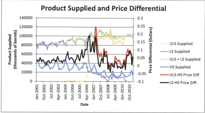
3.5.1. Price History Analysis... 40
3.5.2. Cost Buildup Approach... 42
3.5.3. Cost Distribution...46
3.6. Sensitivity Analysis ... 46
3.6.1. Monte Carlo Analysis Framework... 46
3.6.2. Nom inal Range Sensitivity Analysis ... 47
3.6.3. Global Sensitivity Analysis ... 47
3.7.1. Change in Fuel Properties... 48
3.7.2. Fuel Lubricity...49
Chapter 4: EBCA Results... 52
4.1. Aerosol RF Results... 52
4.2. Mortality Results by Country... 53
4.3. VSL Results by Country... 55
4.4. Global and US ULSJ O utcom es ... 56
4.4.1. Assum ptions for Global and US Im plem entation Analysis ... 56
4.4.2. Assum ed Uncertainty Distributions... 58
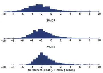
4.4.3. Global Im plem entation Analysis Results ... 61
4.4.4. US Im plem entation Analysis... 62
4.4.5. US-Only Im plem entation Analysis ... 64
4.4.6. Constant VSL Analysis ... 65
4.4.7. Cost Effectiveness Analysis ... 66
4.5. Policy Im plications ... 66
4.6. Nom inal Range Sensitivity Results ... 68
4.6.1. Discount Rate ... 70
4.7. Global Sensitivity Analysis (GSA) Results ... 71
Chapter 5: Fast Policy Analysis... 75
5.1. Adjoint Model and Policy Tool... 75
Chapter 6: Conclusions and Future W ork... 82
6.1. Global ULSJ Implementation...82
6.2. Fast Policy Analysis... 83
6.3. Limitations ... 83
6.4. Future W ork...84
Appendix A: Tables...87 W o rks C ited ... 9 7
List of Figures
Figure 1: Radiative forcing estimates of aircraft emissions... 2
Figure 2: Multi-branch hysteresis behavior of an ammonium sulfate aerosol particle. Plot from W a n g e t a l...1 0 Figure 3: The product supplied of ULS, LS, and HS diesel fuel plotted simultaneously with the price differential for ULS-HS and LS-HS for Jan 2001 to February 2011 ... 41
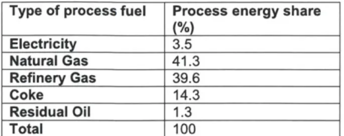
Figure 4: NG Price history required for ULSJ hydroprocessing where prices are presented based on 2.37 scf/gal (0.018 scm/L) of NG per gallon of ULSJ. ... 44
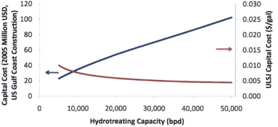
Figure 5: Capital costs for hydrotreating and SMR units as a function of HDS capacity depreciated over 30 years... 45
Figure 6: Benefit-cost distribution for global implementation analysis for three different discount ra te s (D R s ). ... 6 1 Figure 7: Benefit-cost distribution for US implementation analysis. ... 63
Figure 8: Benefit-cost distribution for US-only implementation analysis... 64
Figure 9: Benefit-cost distribution for a constant US VSL analysis. ... 65
Figure 10: NRSA results for global implementation of ULSJ... 68
Figure 11: NRSA results for US implementation of ULSJ. ... 69
Figure 12: Net benefit-cost plotted against discount rate of the deterministic model used in the N R S A ... 7 0 Figure 13: Global Implementation GSA main effect sensitivity index results... 72
Figure 14: Global Implementation GSA total effect sensitivity index results... 72
Figure 15: US Implementation GSA main effect sensitivity index results ... 73
Figure 17: Using sensitivities to compute the total impact from an aircraft emissions policy
s c e n a rio .'...7 6
Figure 18: Forward model premature mortality results from the ULSJ EBCA. ... 77
Figure 19: Adjoint policy tool results and adjusted results for global ULSJ implementation. ... 78
Figure 20: Adjoint policy tool results for monetized avoided premature mortalities with an
assumed income elasticity of 1. ... 80
List of Tables
Table 1: Assumed properties of "sulfates" optical bin in GEOS-Chem... 11
Table 2: On-road implementation timeline of ULSD in the US ... 19
Table 3: Off-road implementation timeline of ULSD in the US.' ... 20
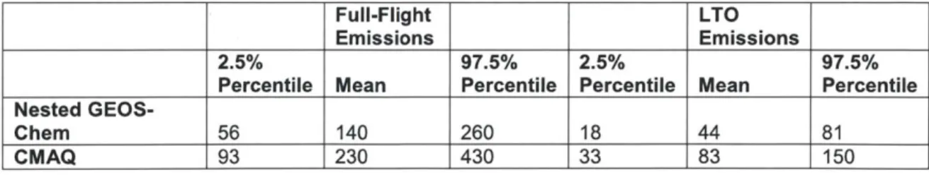
Table 4: Source-receptor mortality impact from full-flight aircraft emissions. ... 24
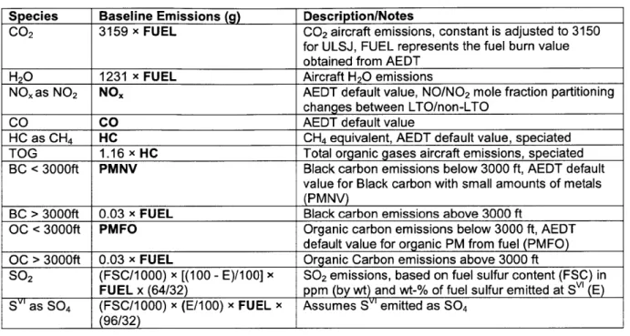
Table 5: Emission indices methodology for air quality simulations, where bolded variables are fro m A E D T . ... 2 7 Table 6: Coefficients in Eq. (11) and associated values and uncertainties. ... 30
Table 7: Percentage increase in avoided mortalities given a 1 pg/m3 increase in ground-level PM2 5 concentration. Values from Pope et al. and Laden et al. ... 38
Table 8: Process energy shares required for jet fuel production... 44
Table 9: Aviation sulfate RF by component and region. ... 52
Table 10: Avoided mortalities by country due to global ULSJ implementation. ... 54
Table 11: Regional simulations avoided mortalities results for the US from global im plem entation of U LSJ ... . . 54
Table 12: VSL and valuation of avoided premature mortalities (when cruise emissions are included) due to ULSJ implementation by country in US 2006 $. ... 56
Table 13: Brief description of each input parameter. ... 59
Table 14: Monte Carlo Input Values and Distributions (Triangular: [Low, High, Nominal])...60
Table 15: Global implementation EBCA results, given in 2006 US $ Billion... 61
Table 16: Global implementation results from EBCA where no implementation cost has been included, given in 2006 US $ Billion. ... 62
Table 17: Global implementation results from EBCA where no climate cost has been included,
given in 2006 U S $ B illion. ... . 62
Table 18: US EBCA results for global implementation, given in 2006 US $Billion. ... 63
Table 19: Valuation of US health impacts due to global implementation from CMAQ and GEOS-C hem N ested sim ulations. ... 63
Table 20: US-only implementation EBCA results, given in 2006 US $ Billion. ... 64
Table 21: Constant US VSL EBCA results, given in 2006 US $ Billion. ... 65
Table 22: Cost effectiveness analysis results, given in 2006 US $ Million. ... 66
Chapter 1: Introduction
While aircraft emissions represent only -1% of total fossil fuel use in the world,' aircraft operations are expected to increase by -5% annually.2 If this growth is realized, current
aviation operations will double by 2025 and represent the fastest growing mode of
transportation. As with any transportation sector, the environmental impact of aircraft emissions is of growing concern. The prioritization of improving air quality is reflected historically in legislation passed within the United States (US), such as the Clean Air Acts of 1970 and 1977,5 which motivated the restrictions placed on allowable pollutant concentrations. With regards to the transportation sector, the US has also required the use of desulfurized diesel fuel for on and
6
off highway purposes to reduce ground-level pollutant concentrations. Similar regulations also exist in many European nations. Specifically regarding aviation, the International Civil Aviation Organization's (ICAO) has routinely recommended increased aviation NOx stringencies to reduce negative health impacts derived from aircraft operations through an improvement in air quality.7
Aircraft emissions have both climate impacts, through their impact on the atmospheric radiative balance, and human health impacts, due to increased ground-level pollution concentrations by way of the chemical reaction of emissions with the ambient atmosphere and vertical transport. Policymakers have placed increased emphasis on mitigating the environmental impacts of aviation where the Federal Aviation Administration (FAA) has defined a set of prospective policy
8
goals in their Destination 2025 plan. This thesis aims to provide a framework in which to evaluate potential aviation policies within the context of a global environmental benefit-cost analysis (EBCA) with an emphasis on quantifying and monetizing air quality and climate impacts in order to achieve these policy goals.
1.1. Aircraft and the Environment
Aircraft emissions are comprised mostly of carbon dioxide (CO2) and water vapor (H20), each
making up 71 % and 28% of emissions, respectively. A small, but significant, portion of these emissions are comprised of nitrogen oxides (NOx), sulfur oxides (SOx), hydrocarbons (HCs), carbon monoxide (CO), and primary PM2.5. PM2.5 refers to particulate matter with a diameter
less than or equal to 2.5 pm, and primary PM2.5 is particulate matter that is directly emitted from
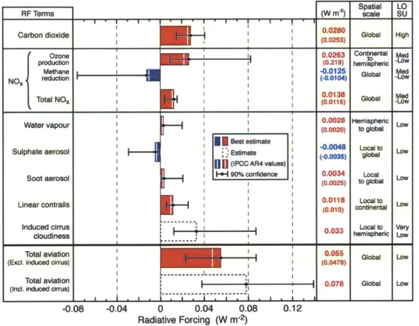
aircraft emissions on the whole have a net warming effect on the atmosphere as estimated based on the most current understanding of how aircraft perturb the state of the atmosphere. Figure 1 shows the estimated radiative forcing (RF) contribution of these emissions as well as species (e.g. aerosols) and phenomena (e.g. contrail formation) derived from aircraft emissions with uncertainties.
I RF Terms
-0.08 -0.04 0 0.04 0.08
Radiative Forcing (W M-2)
0.12
Figure 1: Radiative forcing estimates of aircraft emissions.10
RF is a metric used to quantify the net perturbation to the atmospheric radiative balance from a particular atmospheric species. It is typically taken at its top-of-the-atmosphere (TOA) value, i.e. the net incoming minus the net outgoing radiative flux at the border between the atmosphere and space, although measures at other levels of the atmosphere are also possible. RF is not the only way by which to measure the climate impact of atmospheric species, where global warming potential and integrated temperature change are also common metrics." For the purposes of this analysis, however, RF provides the most convenient impact measure.
(W m2(W m) sale ) Spatial LOSU
Carbon dioxide Global High
Ozone 0.0263 Continental
production (0.219) hemiheric
Methane -0.0125 Global
NOx reduction (-0.0104)
Total NOx 00 Global
Water vapour Hemispheric Low L
I I(0.0020) to global
*lBest estimate
Sulphate aerosol iI
jEstimate
-0.0048 Local to LowS (-0.0035) global
fl
(IPCC AR4 values)Soot aerosol -90% confidence 0.0034 Local OW
(0.002S) to global
Linar ontail I I0.0118 Local to
Linear contrails (0.010) continental LO
Induced cirrus Local to Very
cloudiness 1 hemispheric Low
Total aviation 1 0.055 Global Low
(Excl. induced cirrus) (0.0478)
1..
. .J...Total aviation . 0.078 Global Low
Greenhouse gases (GHGs), such as carbon dioxide (CO2), ozone (03), methane (CH4), and
water vapor, warm the atmosphere. As can be seen from Figure 1, direct emissions of C02 and water vapor both lead to warming as aircraft directly increase the concentration levels of these species, although the net RF impact (where red/positive denotes warming) of C02 is an order of magnitude larger than water vapor. The formation of ozone also leads to a positive RF impact
by way of the NOx cycle:
NO
+034
N0 2+0 2NO2 + hv
+
NO + 0O + 02 + M + 03 + M
NOx emissions, which are primarily NO (except at low thrust), destroy ozone, but can also
produce ozone given the production of NO2. In addition, NO and NO2 are cycled between one another and can result in ozone production and loss through the following reactions:
HO2 + NO -- OH + NO2
H0 2+0 3-+OH+02+0 2
OH + 03 4 HO2 + 02
Thus, ozone formation is a function of not only NOx emissions, but also ambient concentrations of OH and HO2, two very important atmospheric oxidizing agents. Ozone formation is also a
strong function of altitude where ozone production efficiency (i.e. proportion of NOx that is ultimately converted to ozone) is higher at cruise altitudes than at ground-level. NOx molecules also interact with the methane cycle, where aircraft emissions lead to an atmospheric decrease
in methane (thus an associated cooling), but an associated decadal loss of tropospheric ozone leads to further cooling.9 NOx emissions from aircraft that are closer to the ground can either create or destroy 03, and this behavior is a function of the ambient hydrocarbon (HC)
concentration in a particular region.
Aircraft emissions also lead to the formation of primary and secondary aerosols. As mentioned previously, primary BC is a direct emission from combustion and leads to a warming effect. Secondary sulfate aerosols (as well as ammonium nitrate aerosols) are formed from either direct SO emissions or oxidized SO emissions, where inorganic aerosols of this type refract
solar radiation back into space, thus providing a net cooling effect. Linear contrail formation in the wake of the aircraft provides an additional net warming effect. The most uncertain climatic
impacts of aircraft emissions, however, are the induced cirrus cloudiness and soot-cirrus. Cirrus cloud formation is caused by the spreading and shearing of linear contrails as a result of
increased particulate matter concentrations in the atmosphere, which provide nuclei from which clouds can grow. 9 The effect of this indirect climate impact can be either warming or cooling.
Figure 1 shows it as a net warming effect, but with an associated large uncertainty.
Primary and secondary particulate matter is also harmful to human health through ground-level population exposure. Exposure to PM, such as sulfate aerosols and BC, has been shown to lead to increased risk in cardiopulmonary disease (CP) as well as lung cancer (LC), and long-term PM exposure have been associated with overall increases in human premature mortality, where premature mortality comprised approximately 85% of all monetized health impacts from
PM2.5 exposure. Although population exposure to ozone also has human health impacts, it is
not considered in this thesis. In addition, morbidity impacts (hospital admissions, missed work days, etc.) are also not considered.
1.2. Policy Objectives
In their Destination 2025 document, the FAA has stated 6 distinct goals to improve sustainability
8
and reduce the overall impact of aircraft transportation operations by 2018. These goals are the following:
- Reducing those exposed to aircraft noise to less than 300,000 people
- Implementing an alternative fuel for current leaded general aviation fuel
- Improve fuel efficiency by 2% annually
- Reduce the health impacts of aircraft emissions by 50% relative to a 2005 baseline
- Set aviation on a trajectory for carbon neutral growth relative to a 2005 baseline
- Use at least one billion gallons of renewable jet fuel
This thesis focuses primarily on the impact of aviation emissions on the environment and human health, thus topics concerning other aspects of sustainability or aircraft noise reduction will not
be discussed. The major focus of this thesis is, however, on global as well as regional
implementation of an ultra-low sulfur jet fuel (ULSJ), where the emphasis is placed on reducing ground-level PM2.5 concentrations with the ultimate goal of reducing the human health impact of
aviation operations. ULSJ would serve as a drop-in and immediate replacement fuel where rulemaking would mandate a fuel sulfur content of less than 15 ppm by mass.
1.3. Motivation
In order to determine the viability of a particular piece of environmental legislation or rulemaking, standard benefit/cost analysis (BCA) techniques are employed in which potential economic, climate, and health benefits, disbenefits, or societal costs are monetized and aggregated in order to determine a net benefit/cost outcome. The general BCA framework will be discussed in
greater detail in Section 2.4. Analysis currently conducted within the Partnership for AiR
Transportation Noise and Emissions Reduction (PARTNER), such as that performed for the
NO) stringency analysis, is regionally focused on the US, and BCA has only historically
considered landing/take-off (LTO) emissions. A suite of tools known as the aviation environmental portfolio management tool (APMT) has been developed by PARTNER that determine noise, air quality (LTO emissions, only), and climate impacts and monetization of damages of aviation policy scenarios within the US. APMT can assess policies from a US perspective, but does not currently have the ability to account for a global-scale analysis. Barrett et al.,14 however, has shown that cruise emissions have a significant impact on ground-level air quality, where -8000 premature mortalities per year are attributable to aircraft cruise emissions, which constitutes 80% of the total mortality impact derived from all aircraft
emissions. Given the time scale of removal and transport of PM2.5 and its associated precursors,
aircraft emissions then have an inherently global impact. As such, it becomes necessary to adjust the scope of policy analysis to incorporate the global atmospheric impact of a particular aviation policy. This requires global atmospheric modeling through the use of global chemical transport models (GCTMs), rather than only more regional or localized air quality models. In addition to other difficulties, it is also necessary to determine the ground-level health impact in countries outside of the US where epidemiological data may not be available.
The primary goal of this thesis is to expand the analytical capabilities of PARTNER and the
APMT tool suite to include global scale BCA studies of aircraft policy emissions scenarios. This
fuel study where a comprehensive BCA may be necessary to validate or invalidate a transition away from today's standard jet fuel. This requires the development of a comprehensive global environmental benefit/cost analysis framework in which to streamline current and future aviation policy analyses in order to achieve the afore stated FAA policy goals.
1.4. Thesis Structure
This thesis has the following structure:
Chapter 1 generally addresses how aircraft impact the environment and more specifically discusses some of these prospective policy goals and potential aviation policy options. Chapter 2 provides background on general EBCA methodology, including current benefit-cost analysis techniques employed by the Environmental Protection Agency (EPA).
Chapter 3 discusses the EBCA methodology developed for the purposes of global policy analysis, including determining aviation emissions impacts and monetizing these impacts. This is developed within a framework to address the environmental and economic impacts of an ultra-low sulfur jet fuel (USLJ) scenario that would require all commercial jet fuel to have a fuel sulfur content (FSC) of less than 15 ppm.
Chapter 4 presents the results of an EBCA as applied to a case study of global and US implementation of ULSJ.
Chapter 5 extends this policy analysis framework to a discussion of a fast policy tool derived from an adjoint sensitivity analysis. A comparison between the previous EBCA mortality outcomes versus those calculated from the adjoint fast policy tool is also provided.
Chapter 6 presents results from an adjoint sensitivity analysis as applied to temporal variations in aviation emissions impacts and a discussion of the potential policy implications of these variations.
Chapter 2: Background
This chapter provides background information for the EBCA methodology that will be developed in Chapter 3. It includes a discussion on the types of atmospheric models used as well as some basic information concerning how aerosols (i.e. PM2.5) impact the radiative balance of the
atmosphere. In addition, literature is reviewed related to the link between PM2.5 concentrations
and premature mortality risk and current EBCA practices. Information is also presented from an ultra-low sulfur diesel (ULSD) case study that was performed given the similarities between diesel and jet fuel. Finally, a brief description of adjoint sensitivity analysis and how it relates to policy analysis is provided.
2.1. Atmospheric Modeling
EBCA is directly dependent on the ability to chemically and physically model the perturbation to
the atmosphere resulting from anthropogenic emissions. Once emissions scenarios have been accurately defined, it is then necessary to incorporate these scenarios into the appropriate physical models. Two different models are generally employed within PARTNER to conduct air quality studies. On a global scale, GEOS-Chem, a GCTM, is typically used, although the nested version can also be applied to smaller, higher resolution domains. For more local studies (i.e.
US, only), the Community Multiscale Air Quality (CMAQ) model is used. CMAQ has been used by the EPA in their air quality policy analyses, but because CMAQ was used as a sensitivity
study compared to GEOS-Chem and nested GEOS-Chem simulations for the ULSJ analysis, no detailed description will be provided in this thesis.
2.1.1. Global and Nested GEOS-Chem Model Descriptions
GEOS-Chem is a tropospheric model (with an approximated stratosphere) that simulates global gas and aerosol phase chemistry (including aerosols that are relevant to aircraft emissions), accounts for wet and dry deposition, and models transport on an intercontinental scale.15 The model takes in emissions and meteorology as inputs and at the end of each time step computes new tracer concentrations. A typical chemistry time step is 60 minutes and a year simulation with a 3 month spin-up period, which is required to eliminate the impact of the initial conditions, takes approximately 12 hours to perform.
GEOS-Chem generates three dimensional, gridded data. For the ULSJ analysis, a 40 x 50
horizontal grid is typically used, while nested simulations use a 0.5* x 0.6660 horizontal grid
where boundary conditions are provided by the coarser resolution simulation. These simulations also use the GEOS-5 reduced vertical grid that is defined up to 0.01 hPa, where the atmosphere is split into 47 layers. GEOS-Chem also has a built-in aerosol optical property module in which it calculates optical depths of the primary aerosol species, but it currently does not have an
integrated radiative transfer model (RTM) to allow for climate studies. An aircrafts emissions module was previously implemented into GEOS-Chem where species concentrations in the appropriate grid cells were perturbed given aircraft emissions at that location. The model currently allows the user to switch on or off particular aircraft emissions types, to choose to include full aviation emissions or only LTO emissions, and to set the FSC.
2.2. Impact of Aerosols on Climate
Inorganic aerosols, such as ammonium nitrate and ammonium sulfate, scatter incoming solar radiation. In atmospheric models, sulfate aerosols are considered to be purely scattering, i.e. extinction of incoming solar radiation is achieved by only refraction and not through
16
absorption. With sulfate aerosols, the amount of solar radiation that is refracted back into space is determined by a given particle's backscattering coefficient, 0.
1
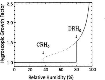
is a function of several parameters, including solar incidence angle and radiation wavelength, but most notably it is a function of particle size.In general, aerosols can exist as a solid or as an aqueous particle. Transition between solid and aqueous states for sulfate aerosols is governed by a hysteresis cycle. In this cycle, aerosol particle radius is a function of relative humidity given the hygroscopic growth (i.e. water vapor condensation) that occurs on the particle, which in turn impacts the optical properties of the particle.17 Thus, an increase in relative humidity can cause an increase in particle radius through
water condensation in order to maintain thermodynamic equilibrium, but this growth behavior is specific to the relative humidity history of the particle. Figure 2 gives an illustration of this hysteresis cycle.
s-. 2.5
DRo
0-0z~
DRH
0 U 0- 1.0CR1-I
0 20 40 60 80 100Relative Humidity
(%)
Figure 2: Multi-branch hysteresis behavior of an ammonium sulfate aerosol particle. Plot from Wang et al."
From Figure 2, there are two distinct pathways that the ammonium sulfate aerosol particle can follow, which are in general called the upper and lower hysteresis branches. In the lower branch (solid line), no hygroscopic growth is experienced until a threshold RH value of 80% (DRHo) is reached if the particle is initially solid. Similarly, an aqueous particle will not begin to crystallize if it exists on the upper branch (dashed line) until a threshold RH value of 35% (CRHo) is reached. Thus, relative humidity history dictates on which branch a given aerosol particle exists given some assumption concerning the initial phase of the particle of interest. In addition, different aerosol types have different hysteresis pathways, which add to modeling complexity when
aerosol mixing ratios need to be determined or assumed.
From this particle growth data as well as total atmospheric burdens, the aerosol optical depth can be calculated, which is a dimensionless measure of the atmospheric burden of the aerosol as it relates to extinction of solar radiation and is mathematically defined as
(x1, x2; 2=f b(x, 2) dx Eq. (1).16
As can be seen in Eq. (1), the optical depth, -r, is a function of the two integration bounds as well as the wavelength of the incoming solar radiation. b is known as the extinction coefficient and is proportional to the burden of the species within the atmosphere as well as the optical properties of that particular species. Optical depth is directly related to the RF contribution of that species.
The methodology implemented for this thesis for RF due to sulfate aerosol scattering is discussed further in Section 3.2.1.
GEOS-Chem takes a simplified approach to the treatment of inorganic aerosols and its calculation of optical depth. GEOS-Chem currently tracks atmospheric burdens of nitrates, sulfates, and ammonium individually, but they are lumped together within the "sulfates" bin when performing optical calculations, where the primary underlying assumption is that the three different species are internally mixed (i.e. mixed aerosols are homogenous). GEOS-Chem, however, does not consider more complex internally mixed aerosols, such as liquid H2SO4
deposited on BC particles. The particle size distributions for dry "sulfates" (i.e. 0% RH) are assumed to be as shown in Table 1.
Table 1: Assumed properties of "sulfates" optical bin in GEOS-Chem.
Property Value
Density 1.7g/cm
Geometric Mean Radius 0.07 pm
Geometric Standard Deviation 1.6
Effective Radius 0.12 pm
Refractive Index 1.43-10-8i
Additionally, the hygroscopic growth behavior of sulfate aerosols within GEOS-Chem is outlined in Martin et al. The assumed refractive index is that of sulfuric acid aerosol and no complex hysteresis behavior is assumed. Different mixing fractions, however, and the impact on the assumed refractive index are not considered and is the subject of ongoing development within the model.
2.3. Air Quality and Mortality
This section contains significant contributions from Dr. Jon Levy from Boston University School of Public Health.
Many studies have linked PM2.5 exposure to adverse health end-points in the US, most notably
the American Cancer Society (ACS) 19,20 and Harvard Six Cities2 cohort studies in which populations were monitored over time and the associations between several health incidences and long-term exposure to ground level PM2.5 concentrations were monitored. For this analysis, only premature mortality is considered given that approximately 85% of all monetized health
avoided mortalities through a concentration-response function (CRF). For this analysis, a linear
CRF is used based on follow-up analyses of the aforementioned cohort studies and an EPA expert elicitation study,23 which comprehensively describes current interpretation of
epidemiological evidence based on expert opinion.
24
Studies, as outlined in Pope et al. provide evidence of a link between premature mortality and long-term exposure to PM2.5. The EPA expert elicitation study2 showed that several leading
experts believe that the main contributors to mortality from short-term exposure are acute cardiac or respiratory events, possibly from pre-existing health conditions. Mortality due to long-term exposure is most likely a result of cardiovascular disease, chronic respiratory disease, and lung cancer. The biological drivers of these premature mortalities are still uncertain, although it is strongly believed that PM exposure can lead to health issues such as chronic obstructive pulmonary disease (COPD)25,26 and atherosclerosis.27 An impact on lung cancer risk due to PM exposure is thought to exist, but the relationship remains uncertain as compared to
cardiopulmonary illnesses,28,29,30 although relative risks have been calculated for lung cancer. Given these established links to human health, deaths resulting from cardiopulmonary (CP) diseases and lung cancer (LC) are assumed to be the dominating health impact pathways given a change in ground-level PM2.5 concentrations. Uncertainties for each disease are captured in a
range of relative risk values obtained through literature review.
A linear CRF is assumed given the results from multiple analyses of long-term studies. In addition, no substantial evidence has been found for a concentration level at which health
24 31
impacts exhibit a significantly different concentration response. Specifically, Schwartz et al.
conducted an analysis that included threshold and non-linear models, and also concluded that a linear fit does indeed best fit the data. This interpretation concerning CRF shape is also
reiterated within the EPA expert elicitation study. Nonlinearities are observed, specifically in the Pope ACS cohort analysis. Goodness-of-fit tests, however, have shown that the probability of a non-linear fit being statistically different from that of a linear fit is not significant.24 These cohort studies, however, did not consider very high pollutant concentration levels that may be seen in portions of the developing world (-50 pg/m3 versus -10 pg/m 3 in the US). In these cases, the
assumption of a linear CRF may be inappropriate as the marginal impact of pollution at very high concentration levels may be decreasing and the number of premature mortalities predicted may be overestimated. To account for this, the CRF applied in Ostro86 as part of a World Health Organization (WHO) study assumes a log-linear relationship with changes in concentrations,
which results in a lower premature mortality response at higher background PM2.5
concentrations.
Differential toxicity among PM2.5 species is a subject of ongoing research and is relevant given
that the change in ground-level PM2.5 due to ULSJ implementation is seen primarily in S04
species. The relative impact of S04 species on air quality becomes important in determining the
32
magnitude of avoided mortalities seen due to a reduction in FSC. Hedley et al. showed that a reduction in SOx emissions in Hong Kong due to a sulfur content restriction of 5000 ppm for fuel used in power plants and road vehicles led to 80% and 41% reductions in S02 pollution and SO4 particulate concentrations, respectively. This improvement in overall air quality was
accompanied by a 2.1% reduction in all-cause mortality, a 3.9% reduction in respiratory disease related mortalities, and a 2.0% reduction in cardiovascular related mortalities in annually
averaged trends after the fuel regulation was enforced. In addition, some studies have shown a link between sulfate aerosols and CP related health incidences,3 3 343 5 , and committees have concluded that there is currently not enough evidence to discredit the assumption of equal
toxicity. 53,36
More recent results presented by Levy et al.,37 where a probabilistic analysis was applied to determine the relative toxicity of constituent species relative to PM2.5 as a whole, however, show
that sulfate has only a 42.7% of being more toxic than PM2.5 with regards to cardiopulmonary
illnesses. This is in stark contrast to elemental carbon and nitrate, which have a 100% and
97.7% chance of being more toxic than PM2.5. Probabilities are lower in general for respiratory
illnesses. Levy et al.,37 however, does acknowledge the large uncertainty present in this analysis and state that the results only suggest the possibility of differential toxicity. In this thesis, differential toxicity is not directly considered and all PM2.5 species, including those
derived from SOx emissions, are assumed to have equal health impacts. This is, however, a significant uncertainty.
2.4. Elements of EBCA
For the purposes of this thesis, many of the guidelines set by the EPA have been incorporated into the techniques employed within this particular analysis. This section will serve as a brief overview of these practices and any assumptions that were required when these guidelines
2.4.1. Benefit/Cost Analysis
BCA (or also commonly, CBA) is a general framework in which policy analysis is commonly
performed. It requires the identification of both benefits and costs, each of which can be positive or negative for society (negative benefits are also referred to as "disbenefits"). Distinguishing
between benefits and costs is, in some cases, not always straightforward. For the case of environmental policy analysis, a general rule of thumb is that positive or negative outcomes derived from the actual implementation of a policy fall under the benefits category (e.g. decrease in premature mortality or increase in climate damages) while costs are assigned towards the actual implementation of the policy, be it the need for additional infrastructure, land, etc.
Furthermore, BCA requires a definition of both a baseline and policy scenario. Within aviation policy, the baseline scenario has been defined using aviation in the year 2006 where the most complete set of aircraft emissions inventory data available. The policy scenario is then defined relative to this baseline aviation scenario. As an example, the ULSJ policy scenario would have aircraft SOx emissions reduced by a factor of 15/600, where this factor is the ratio of the
proposed FSC of 15 ppm to the current average FSC of 600 ppm. As the atmosphere is a highly nonlinear system, the definition of the background emissions, i.e. emissions from all other sources not including aviation, is also important for both the baseline and policy scenario
outcomes. As the focus of this thesis is on aviation policy, the topic of background emissions will not be addressed in detail, but a brief description of the source for these background emissions is provided in Section 3.
Sensitivity analysis and uncertainty quantification also play a vital role in BCA. From the
atmospheric modeling to metric monetization, policy analysis is a highly uncertain process. This is due in large part to the limitations of the physical models used and, particularly for
environmental analysis, the lack of real markets in which to obtain monetary values that can be easily assigned to climate damages or premature mortalities. As such, it becomes necessary to utilize Monte Carlo techniques in order to provide both a policy outcome distribution as well as a comprehensive sensitivity analysis to determine the primary sources of uncertainty given the assumptions within the analysis.
2.4.2. Discounting
A key component of BCA is the discounting of all future benefits/costs. In an economic sense,
money now is worth more to a person than money in the future and the degree to which a person experiences that opportunity cost is contained within the discount rate, which is directly tied to the concept of a net present value (NPV). NPV is defined in the following equation:
NPVCt Eq.(2) t1(1 +r)t
where Ct is the cash flow for that time period, t is the time period, and r is the discount rate. Within the base year of the analysis, the time period is 0 (i.e. costs in the initial year of a policy are not discounted). The cash flow can be defined as the relevant benefit or cost quantity within that time period. The US government has identified a range of appropriate discount rates
(2-7%)38 to be applied in BCA, where this range is also applied for aviation environmental policy
analysis. The higher the discount rate, the more current costs are valued against future costs, and vice versa. Thus, different choices in discount rate will cause different policy assessment outcomes, especially when the time scales of benefits and/or costs are significantly different. Discounting plays an important role in valuing both climate damages as well as human health impacts. Aviation emissions in a given year can have impacts out to hundreds of years, thus it becomes necessary to take the NPV of all costs over a time horizon that captures these impacts to fully quantify the climate benefit/disbenefit associated with a given policy scenario. In the case of climate damages, Eq. (2) can be directly applied where the cash flow for a specific year is the climate damage in that year, all of which is computed within APMT. A more detailed description of how APMT assigns climate damages will be discussed in Section 3.2.5.
As suggested by the EPA, it is also necessary to discount health impacts based on a prescribed lag schedule. It assumes that 30% of avoided mortalities are seen in the year of implementation,
50% in years 2-5, and the remaining 20% spread out over years 6-20.39 The assumed discount
rate can then be applied to each year as required, and then premature mortalities can be summed over the full 20 years to obtain a "discounted" premature mortality outcome. This thesis applies the same discount rate for all discounting purposes as the EPA does not provide any insight on application-specific discount rates.
2.4.3. Premature Mortality
Based on the information presented above, the EPA recommends the use of a linear CRF with a nominal estimate of 1.06% for the CRF coefficient. A Weibull distribution was assumed for the
CRF coefficient within The Benefits and Costs of the Clean Air Act from 1990 to 2020,39 but no distribution parameters were provided. For this thesis, upper and lower bounds were determined from the EPA expert elicitation study concerning CRFs.
2.4.4. Valuing Lives
Valuing premature mortalities is a very complex issue, both from an economic as well as social justice perspective. The US recommends that the value of a statistical life (VSL), largely calculated from wage-risk studies, be applied in matters of policy analysis when mortality
monetization is required. As this tends to be a sensitive issue within policy analysis, a brief overview of VSL use standardization within the US is provided below.
Standardizing VSL use within US cost-benefit analyses was first addressed in OMB Circular
A-4.40 A literature review concluded that the "substantial majority of the resulting estimates of VSL
vary from roughly $1 to $10 million per statistical life." Based on a review by the EPA's science advisory board (SAB), two important conclusions were drawn: it is appropriate to adjust VSL relative to income and a lag structure for health effects should be applied. OMB advised a standard value of $5 million, but acknowledged the value was lower than other estimates in federal agencies, specifically the EPA.
In DOT's 2009 VSL guidance memorandum,4 1 the standard estimate applied within DOT was
updated from a previous value provided in a 2008 memorandum. In this update, five different
US VSL studies were taken and adjusted for real income growth (with an assumed income
elasticity of 0.55 based on a literature review) as well as inflation using the consumer price index (CPI). $5.8 million was given as the mean value adjusted to 2007 prices. While the original OMB range of $1 to $10 million was not ruled out, DOT suggested a more specific uncertainty range of $3.2 to $8.4 million. A normal distribution with a standard deviation of 2.6 million was recommended, although due to the unrealistic negative values that this
encompassed, other distributions, such as Weibull or lognormal, were also recommended, but no distribution parameters are provided. In terms of policy applications, DOT stated "the same standard is to be applied to all individuals at risk, regardless of age, location, income, or mode
of travel," thus setting requirements that all individuals within the US be monetized by the same
VSL.
In EPA's Guidelines for Preparing Economic Analyses,38 a central estimate of VSL is given as
$7.4 million. This value is based on 26 VSL studies. VSLs are adjusted year to year by a GDP deflator, although it appears that no adjustment is made for real income growth or decline. A Weibull distribution was then fit to these 26 studies, resulting in a scale parameter of 7.75 and a shape parameter of 1.51. The EPA lists several limitations to the provided estimate, including its lack of specificity to environmental hazards, as is true of all current VSL estimates. It concludes that for now, the abovementioned central estimate is the most appropriate estimate of US VSL and should be applied uniformly without the consideration of differences of income within the
US.
In order to be consistent with previous analyses conducted on the impact of changes in air quality on human health, the EPA approach was applied in both calculating and monetizing avoided premature mortalities. Due to the global scope of this thesis, differentiating between premature mortalities in different regions in the world by applying different VSLs could be interpreted to suggest that a person's life in a higher income country is "worth" more than a life in a lower income country. Heinzerling42 argues that VSL is in fact an inappropriate valuation to apply to premature mortalities as it does not capture the value of lost (or saved) life but rather just the value of the increased risk associated with a more "unsafe" environment. In this thesis,
country specific VSLs are applied, and the justification for this approach is provided in Section
3.3, although a constant VSL approach is also applied as a comparison.
One of the disadvantages of using VSL as a mortality monetization metric is that it does not capture the temporal aspect of when the premature mortality occurs. For instance,
complications from CP illnesses may place the elderly at much greater risk than younger members of the population, but a premature mortality from either age group is valued equally. Thus, an alternative metric, as applied in the ExternE43 study, is the value of lost life years (VOLLY). This involves calculating the expected age of mortality relative to a reference life expectancy, and then monetizing each of the years "lost" due to premature mortality. Although this helps resolve the temporal issue related to the VSL, this approach is not applied in this thesis given the lack of data related to value of a life year lost on a disease specific basis as well
2.4.5. Cost Analysis
Here it is important to distinguish between a financial BCA, in which "real" prices are analyzed, versus a societal BCA, in which the "true" costs seen by society are analyzed.4 As
environmental BCA certainly falls under the latter category, it is necessary to obtain the "shadow" prices (i.e. prices that are not distorted by market effects) when determining the cost of policy implementation. An example of a market distortion might be the oligarchical pricing effect due to the small number of firms within the oil refining industry. As such, the cost analysis
portion of this thesis attempts to determine the "true" costs seen by society as a result of the implementation of ULSJ through both a top-down and bottom-up approach.
2.5. Ultra-Low Sulfur Fuels
2.5.1. Ultra-Low Sulfur Diesel Case Study
Given the similarities between diesel and jet fuel,45 ultra-low sulfur diesel (ULSD)
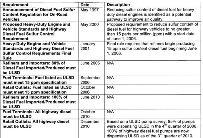
implementation within the United States was used as a comparative case study for ULSJ, especially for the cost analysis. ULSD, through EPA rulemaking, was phased-in to production for on and off-road uses. Table 2 shows the timeline for on-road implementation of ULSD, while Table 3 shows the timeline for off-road implementation of ULSD. US implementation of ULSD exhibited a pattern of a gradual increase in fuel sulfur content (FSC) stringency as the fuel
passed from refineries to retail outlets. This implementation was seen over a time period of 10 years for both on and off-road uses.
Table 2: On-road implementation timeline of ULSD in the US.46,47
Requirement Date Description
Announcement of Diesel Fuel Sulfur May 1997 Reducing sulfur content of diesel fuel for
heavy-Content Regulation for On-Road duty diesel engines is identified as a potential
Vehicles pathway to improve air quality.
Proposed Heavy-Duty Engine and May 2000 Proposed requirement to reduce sulfur content of
Vehicle Standards and Highway diesel fuel for highway vehicles to no greater Diesel Fuel Sulfur Control than 15 parts per million (ppm) with a start date
Requirement of June 1, 2006.
Heavy-Duty Engine and Vehicle January Final rule requires that refiners begin producing
Standards and Highway Diesel Fuel 2001 15 ppm sulfur content diesel fuel beginning June Sulfur Control Requirements Final 1, 2006.
Rule
Refiners and Importers: 80% of June 2006 N/A Diesel Fuel Imported/Produced must
be ULSD
Fuel Terminals: Fuel listed as ULSD September N/A must meet 15 ppm specification 2006
Retail Outlets: Fuel listed as ULSD October N/A must meet 15 ppm specification 2006
Refiners and Importers: 100% of June 2010 N/A Diesel Fuel Imported/Produced must
be ULSD
Fuel Terminals: All highway diesel October N/A
must be ULSD 2010
Retail Outlets: All highway diesel December Based on a ULSD pump survey, 85% of pumps must be ULSD 2010 were dispensing ULSD in the 4 th quarter of 2006.
100% of highway diesel fuel pumps are now
Table 3: Off-road implementation timeline of ULSD in the US.46,47
Requirement Date Description
Proposed Clean Air Non- April 2003 Reduce diesel fuel sulfur content to a maximum of
Road Diesel Rule 500 ppm starting in 2007 for non-road applications
(including locomotive and marine applications). Reduce diesel fuel sulfur content to a maximum of
15 ppm by 2010.
Final Clean Air Non-Road May 2004 Non-road diesel fuel sulfur content must be
Diesel Rule reduced from current levels (about 3000 ppm) to
15 ppm by 2010.
Refiners and Importers: Non- June 2007 Fuel must meet 500 ppm standard.
Road, Locomotive, and Marine Fuel
Fuel Terminals: Non-Road, August 2007 Fuel must meet 500 ppm standard.
Locomotive, and Marine Fuel
Retail Outlets: Non-Road, October 2007 Fuel must meet 500 ppm standard.
Locomotive, and Marine Fuel
Refiners and Importers: Non- June 2010 Fuel must meet 15 ppm standard.
Road Fuel
Refiners and Importers: June 2010 Fuel must meet 15 ppm standard.
Locomotive and Marine Fuel
Fuel Terminals: Non-Road August 2010 Fuel must meet 15 ppm standard.
Fuel
Fuel Terminals: Locomotive August 2012 Fuel must meet 15 ppm standard.
and Marine Fuel
Retail Outlets: Non-Road October 2012 Fuel must meet 15 ppm standard.
Fuel
Retail Outlets: Locomotive October 2012 Fuel must meet 15 ppm standard.
and Marine Fuel
2.5.2. QinetiQ Report on Jet Fuel Sulfur Limit Reduction
A report by QinetiQ48 addressed ULSJ implementation in Europe. It estimated that due to the
additional hydroprocessing required, there will be a 0.01 to 0.015 EUR/liter additional required cost in ULSJ production, which is approximately 4 to 7 cents (2006 US$) per gallon. The report also outlined many of the potential impacts the additional hydroprocessing would have on fuel properties as well as operational effects due to the reduction in fuel sulfur content. Potential climate impacts were described, but were not quantified. SO2 emissions as a function of FSC
were estimated for a representative local airport by scaling against a previous dispersion model study at Heathrow Airport49 based on emissions derived from the First Order Approximation methodology.50 The report concluded there is unlikely to be any measurable health effect due to
FSC reduction when only LTO emissions are considered. Full-flight emissions impacts were not
2.5.3. Energy Information Administration (EIA) Report on Market Effects Due to ULSD
An EIA report from 200151 analyzed the possible effects of ultra low sulfur diesel (ULSD)
implementation on the diesel fuel market within the US. Based on a cost curve analysis, a 6.5 to
8.2 (2006 US$) cent/gal marginal cost increase for ULSD production was estimated to cover
additional capital and hydrotreating costs for an assumed future supply and demand. In comparison, the EPA52 predicted a full compliance US average cost of 5.2 cents/gal (2006
US$).
2.5.4. Other Transportation Sectors
Marine fuels have also received significant attention in terms of their global air quality impact.
A policy analysis performed by Corbett and Winebrake53 estimated a 70 to 85% reduction in marine SO,, emissions due to marine gas oil (MGO) and marine diesel oil (MDO) implementation (lower sulfur alternatives) over the standard marine residual oil (RO). Additional C02 emissions were estimated to be less than 1%. In a human health policy analysis, Winebrake et al.54 estimated the total health impacts due to a global marine fuel sulfur content limit. Findings showed a 41,200 reduction in premature mortalities for a global fuel sulfur content limit of 5000 ppm as compared to 87,000 premature mortalities with the assumed baseline emissions scenario. Marine fuel use is defined as an off-road diesel fuel and all marine fuel must meet the
15 ppm standard by the end of 2012, as outlined in Table 3, for all US marine applications
except for RO used by ocean-going ships.
2.6. Role of Sensitivity Analysis
In general, sensitivity analysis is a useful tool to supplement policy analysis. In the case of performing large scale atmospheric chemistry simulations, sensitivity analysis allows for the determination of perturbations to atmospheric concentrations given a small perturbation in emissions without the need to completely rerun entire GCTM simulations. For GCTMs in
particular, however, sensitivity calculation to emissions is not always a simple task, either due to model complexity or excessive computation time. Sensitivity analysis begins by the definition of a cost function, J, which can be any function of the inputs to a given model. For instance, one can define the cost function of a GCTM simulation to be the total atmospheric concentration of a particular trace gas (e.g. ozone) or aerosol (e.g. sulfate) at the final time step, N, of the
emissions in each of the time steps (i.e. 1 to N) on the atmospheric concentration of a particular species in the final time step.
There are two primary methods by which sensitivities can be calculated. In the forward calculation, each input is perturbed individually, and for each perturbation, a simulation is performed to determine the impact on the defined cost function, J. While simple, this approach very quickly becomes computationally expensive given the number of forward model
simulations required. For GCTMs such as GEOS-Chem, a forward calculation of sensitivities for just one particular emission would require the number of forward simulations equal to the
number of grid boxes times the number of time steps. In a standard GEOS-Chem simulation performed for this thesis, there are a total of 72 x 46 x 47 grid boxes (155,664) and within a
year simulation, there are 8,760 time steps, where the standard time step for emissions is 60 minutes. Given that a single year long simulation takes about 12 hours to complete, this problem then becomes far too large given the relatively limited computational resources available.
An alternative procedure for sensitivity calculation is the adjoint method, which has already been implemented within GEOS-Chem. Adjoint methods take a "backward integration" approach to sensitivity calculation. First, the governing equations of the GCTM are linearized so that the following approximation holds true:
Ax" = xn+ Eq. (3),
where A represents the approximate linear operator, xn is the input vector (i.e. grid concentration values) for the current time step, and x"*< is the output vector (i.e. grid concentration values to
serve as inputs in the next time step). As mentioned previously, the cost function, J, can be defined in terms of the output, x''. In that case, the perturbation to J, or 5J, can be computed
by the following relationship:
SJ
= J xn+1Eq. (4),
axn+l
where the transpose notation is a result of the matrix multiplication required given that x is a vector input. From Eq. (3), given that it is a linear approximation, small perturbations in the output can be calculated from the following equation:
Substituting Eq. (5) into Eq. (4) and rearranging some of the notation, the following relationship is obtained:
SJ =AT ] Sx" Eq. (6).
Equivalently, Eq. (4) can be written in terms of sensitivity to inputs:
6J
= 6x' Eq. (7).axn
Comparing Eq. (6) to Eq. (7), the first order derivative becomes
a = A T Eq. (8),
where it can be observed that
A =axni
Eq. (9),
which, based on the previous definitions, is the Jacobian of the system. From Eq. (8), it is then clear that the sensitivity of the cost function to concentrations in previous time steps can be calculated iteratively by multiplying the sensitivity at the current time step by the Jacobian evaluated at that time step. Determining the Jacobian can be a difficult task if the GCTM is inherently complex or poorly organized, where substantial understanding of the underlying code structure is required to implement the adjoint method. The primary advantage to this
"backwards" approach, however, is the wealth of sensitivity data obtained from a single adjoint simulation. It is possible to obtain full 3-D sensitivity data, as well as temporal sensitivity data, for, in the case of GEOS-Chem, an approximate 2.5 times increase in runtime over a standard forward model simulation. These equations are relevant for discrete adjoint method
implementation. The topic of continuous adjoint methods will not be discussed in this thesis. Given that the adjoint method has been implemented within GEOS-Chem, there is considerable freedom in how J is defined. Currently, GEOS-Chem is only compatible with cost functions that are first order differentiable to the outputs. For instance, the cost function can be the total atmospheric ozone burden in the final time step or, alternatively, in all time steps. Thus, J is a sum of the ozone mass in every grid cell over the appropriate time horizon, which is first order differentiable given it is a linear cost function. J can also be defined as a weighted sum of