Complex modulus test protocol and procedure for determining Huet-Sayegh Model parameters

(1)

Publisher’s version / Version de l'éditeur:

Vous avez des questions? Nous pouvons vous aider. Pour communiquer directement avec un auteur, consultez la

première page de la revue dans laquelle son article a été publié afin de trouver ses coordonnées. Si vous n’arrivez pas à les repérer, communiquez avec nous à [email protected].

Questions? Contact the NRC Publications Archive team at

[email protected]. If you wish to email the authors directly, please see the first page of the publication for their contact information.

https://publications-cnrc.canada.ca/fra/droits

L’accès à ce site Web et l’utilisation de son contenu sont assujettis aux conditions présentées dans le site LISEZ CES CONDITIONS ATTENTIVEMENT AVANT D’UTILISER CE SITE WEB.

Internal Report (National Research Council of Canada. Institute for Research in Construction), 2006-11-06

READ THESE TERMS AND CONDITIONS CAREFULLY BEFORE USING THIS WEBSITE. https://nrc-publications.canada.ca/eng/copyright

NRC Publications Archive Record / Notice des Archives des publications du CNRC : https://nrc-publications.canada.ca/eng/view/object/?id=c784ad5d-9879-4c0f-a141-0d9e5e66ff4c https://publications-cnrc.canada.ca/fra/voir/objet/?id=c784ad5d-9879-4c0f-a141-0d9e5e66ff4c For the publisher’s version, please access the DOI link below./ Pour consulter la version de l’éditeur, utilisez le lien DOI ci-dessous.

https://doi.org/10.4224/20378002

Access and use of this website and the material on it are subject to the Terms and Conditions set forth at Complex modulus test protocol and procedure for determining Huet-Sayegh Model parameters

(2)

Com plex M odulus Te st Prot oc ol a nd

Proc e dure for De t e r m ining H ue t -Sa ye gh

M ode l Pa ra m e t e rs

I R C - I R - 8 7 1

Adams, Y.E.; Zeghal, M.; ElHussein H. Mohamed

N o v e m b e r 6 , 2 0 0 6

(3)

FILE PATH:

C:\Documents and Settings\Libcirc\Local

Settings\Temporary Internet Files\OLKD\Complex Modulus Testing Protocol_Rev#1_Nov-2006.doc

THIS DOCUMENT IS NOT CONTROLLED, UNLESS THE ABOVE QA SIGNATURE IS IN RED INK.

PAGE 1 OF 22

1. APPROVALS

The following approvals were obtained prior to issuance of this work instruction as an internal document in Feb. 2006 and again in Nov. 2006 when this document was released as an external publication.

Yassin E. Adam Nov. 06, 2006

Morched Zeghal Nov. 06, 2006

ElHussein H. Mohamed Nov. 06, 2006

Prepared by: Date

Omran Maadani Nov. 06, 2006

Reviewed by: Date

Yehuda Kleiner Nov. 06, 2006

Program Director Date

James Crawford Nov. 06, 2006

Quality Assurance Manager Date

2. SCOPE

This document describes procedures for determining the complex modulus and phase angle of compacted asphalt concrete samples over a range of pavement temperatures and loading frequencies. Also included is a procedure for determining parameters of the Huet-Sayegh model used in NRC’s analytical model for analysis and design of flexible pavements. This procedure is applicable to laboratory-prepared specimens of mixtures with nominal maximum size aggregate less than or equal to 19 mm (0.75 in).

Disclaimer: This standard does not address safety issues and problems associated with its use. Establishing appropriate safety and health practices and determining the applicability of regulatory limitations rely solely on the user of this standard.

(4)

FILE PATH:

PAGE 2 OF 22

3. REFERENCES 3.1 ASTM Standards

• D3496 Method for Preparation of Bituminous Mixture Specimens for Complex Modulus Testing

• D3549 Standard Test Method for Thickness or Height of Compacted Bituminous Paving Mixture Specimens

• D3515 Specification for Hot-Mixed, Hot-Laid Bituminous Paving Mixtures • D2041 Maximum Specific Gravity and Density of Bituminous Paving Mixtures 3.2 AASHTO Standards

• TP4 Standard Method for Preparing and Determining the Density of Hot Mix Asphalt (HMA) Specimens by Means of the SHRP Gyratory Compactor

• PP2 Practice for Mixture Conditioning of Hot Mix Asphalt (HMA)

• T269 Percent Air Voids in Compacted Dense and Open Bituminous Paving Mixtures • T209 Maximum Specific Gravity and Density of Bituminous Paving Mixtures

• T166 Bulk Specific Gravity of Bituminous Paving Mixtures Using Saturated Surface-Dry Specimens

4. TERMINOLOGY

4.1 Definitions:

4.1.1 Dynamic Modulus: The absolute value of the complex modulus that defines the elastic properties of a linear viscoelastic material subjected to a sinusoidal loading, E . *

4.1.2 Complex Modulus: A complex number that defines the relationship between stress and strain for a linear viscoelastic material, E*.

4.1.3 Storage Modulus: The real part of the complex modulus that represents the elastic contribution of the bituminous mixture behavior, E1.

(5)

FILE PATH:

PAGE 3 OF 22

4.1.4 Loss Modulus: The imaginary part of the complex modulus that represents the viscous contribution of the bituminous mixture behavior, E2.

4.1.5 Linear Material: A material whose stress to strain ratio is independent of the loading stress applied.

4.1.6 Phase Angle: A value that shows time dependency of asphalt materials and defines the lag between applied strain and the resulting stress.

4.1.7 Linear Viscoelastic

:

_{Within the context of this test method, it refers to bituminous}

behavior in which the complex modulus is independent of stress or strain amplitude.

5. SUMMARY OF TEST PROCEDURE

This is a strain-controlled test. A sinusoidal axial deformation (tension and compression) corresponding to 120 microstrain is applied at a given temperature and loading frequency. The resulting axial stress is measured and used together with the applied strain to calculate the dynamicmodulus, and then the phase angle.

6. SIGNIFICANCE

6.1 The value of the dynamic modulus reflects the stiffness of the mixture and its resistance to deformation at a designated frequency and temperature. It can be used for mix design and analysis of the asphalt concrete layer of a road.

6.2 Dynamic modulus values measured over a range of temperatures and frequencies of loading can be shifted into a master curve that can be utilized for performance analysis using analytical models.

7. APPARATUS

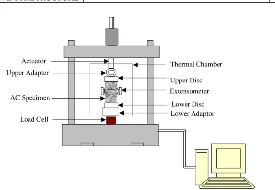
The Dynamic Modulus Test System consists of a loading frame, environmental chamber, measuring systems, and a personal computer (see Figure 1).

(6)

FILE PATH:

THIS DOCUMENT IS NOT CONTROLLED, UNLESS THE ABOVE QA SIGNATURE IS IN RED INK. PAGE 4 OF 22 Thermal Chamber Lower Disc Load Cell Actuator AC Specimen Upper Adapter Lower Adaptor Extensometer Upper Disc

Figure 1: Test set-up

7.1 Loading Frame: A servo-hydraulic testing machine capable of applying an axial sinusoidal strain load over a range of frequencies from 0.1 to 20 Hz and measuring stress level up to 6.0 MPa (800 psi). The guidelines presented in this test protocol have been developed based on the use of the MTS Test Star II System 810. Slight differences may be noticed if a different loading system is used.

7.2 Temperature Control System: A chamber for controlling the specimen at the desired temperature during the test. The environmental chamber must be capable of controlling the temperature of the specimen over a temperature range from -10 to 40 °C (14 °F to 104 °F) to an accuracy of ± 0.5 °C (1 °F). The chamber shall be large enough to accommodate the test specimen and the measuring devices and other accessories.

7.3 Measurement System: A computer-controlled system capable of measuring and recording the time history of the applied deformations, and the corresponding axial load is required.

The system must be capable of measuring the period of the applied sinusoidal deformations and resulting load. The measurement system consists of the following components.

(7)

FILE PATH:

PAGE 5 OF 22

7.3.1 Load Cell:The load shall be measured with an electronic load cell in contact with one of the hardened steel discs through steel adaptor. It is recommended that the load cell be placed in contact with the lower hardened steel disc beneath the specimen. It was found that force measurements are more accurate when the load cell is not in contact with the moving actuator (see proposed position in Figure 1). The load measuring system capacity shall not be less than 45 kN (10 kips).

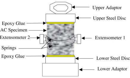
7.3.2 Strain Measurements: The applied axial deformations shall be measured using two extensometers capable of reading deformations corresponding to 120 microstrain. The strain measuring sensors should be mounted with springs on the side of the sample at mid-height (opposite to each other) placed 180° apart (see Figure 2).

7.4 Hardened Steel Disk: Hardened steel disks, with a diameter equal or greater than that of the test specimen are required at the top and bottom of the specimen to transfer the load from the testing machine to the specimen (see Figure 2).

7.5 End Treatment: Friction reducing end treatments shall be placed between the specimen ends and the hardened steel disks. The end treatments shall consist of 0.5 mm (0.02 in) thick epoxy at both ends (see Figure 2).

Upper Adaptor

Extensometer 1 Upper Steel Disc

Lower Steel Disc Lower Adaptor Springs AC Specimen Epoxy Glue Extensometer 2 Epoxy Glue

(8)

FILE PATH:

PAGE 6 OF 22

7.6 Gyratory Compactor: A gyratory compactor and associated equipment is used to prepare specimens in the lab in accordance with AASHTO TP4.

8. SAMPLE PREPARATION

8.1 Mix Type: Follow local specifications. 8.2 Binder Type: Follow local specifications. 8.3 Binder Content: Follow local specifications.

8.4 Size: Size of specimen is determined according to ASTM Designation D 3549. For this protocol, samples having a diameter of 100 mm (4 in) and a height of 100 mm (4 in) are used. 8.5 Mixing: Follow local specifications.

8.6 Aging: Mixtures shall be aged in accordance with the short-term oven aging procedure in AASHTO PP2.

8.7 Compaction: Compact specimens according to AASHTO TP4 or ASTM D3496 to produce the appropriate size at the locally specified air voids percent.

8.8 Physical Properties: The bulk specific gravity, maximum specific gravity and air voids shall be determined according to AASHTO T 166, T 209 and T 269 respectively. Air voids shall satisfy local requirements.

8.9 End Preparation: The ends of all test specimens shall be smooth and perpendicular to the axis of the specimen. Preparation of the ends of the specimen can be achieved by sawing with a single or double bladed saw.

8.10 Sample Storage: Wrap completed specimens in polyethylene and store them in an environmentally protected storage area at temperatures between 5 and 25°C (40 and 75°F). To eliminate effects of aging on test results, it is recommended to select a manufacturing date meeting the testing schedule, which may include a similar storage period prior to testing for all samples that represent different testing conditions.

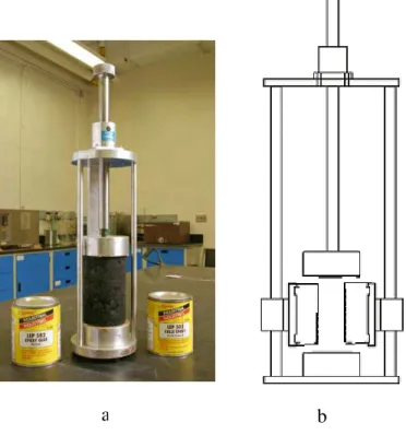
8.11 Glueing: Glue the upper and lower discs to the specimen using an epoxy and leave them to dry for a minimum of 8 hours prior to testing. Pelco LEP 502 Epoxy Glue was found to be effective. The system used to glue the sample is shown in Figure 3.

8.12 Attachment of Strain Gauges: Attach the extensometers with springs to the sides of the specimen near mid-height to measure applied axial strains as shown in Figure 2

(9)

FILE PATH:

PAGE 7 OF 22

8.13 Number of Replicates: The number of test specimens required should be determined based on variations observed in the physical properties of the compacted specimens. A minimum of two specimens is recommended for determining the complex modulus parameters.

Note 1: When connecting gauges to specimens with large-size aggregates, care must be taken so that the gauges are attached over areas between the aggregate faces.

a b

Figure 3: a) System used to glue the sample, b) Handling system details

9. TESTING SYSTEM PREPARATION

9.1 Calibration: All sensors connected to the system should be calibrated. Calibration ensures that the outputs of the sensors accurately represent the physical condition sensed by the device (e.g., displacement or force). The System software manual provided by the manufacturer should be used as a guide for performing all calibrations.

(10)

FILE PATH:

PAGE 8 OF 22

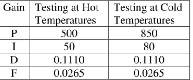
9.2 Tuning: Tuning optimizes test performance by minimizing the system error in the assigned control mode. It also affects the response of the machine in order to produce the exact value of input, and it helps in producing a clear signal. The control extensometer should be properly tuned. Retuning the response of the system may be needed in case the characteristics of the specimen change. The System software manual provided by the manufacturer should be used as a guide for tuning.

Two sets of tuning parameters are created: (a) one for testing at temperatures including -10, 0, and 20°C (14, 32, and 68°F); and (b) another for testing at temperatures including 30 and 40°C (86 and 104°F). Proposed sets of tuning parameters are given in Table 1. Sets more compatible with a local mix, other than those shown in Table 1, may be needed.

Table 1: Typical extensometer tuning parameters Gain Testing at Hot

Temperatures Testing at Cold Temperatures P 500 850 I 50 80 D 0.1110 0.1110 F 0.0265 0.0265

9.3 Computer Program for the Test Protocol: Utilizing the built-in, Multi-Purpose Testware (MPT) software provided by the manufacturer, a computer program should be established to automate the application of the test protocol. The software defines the activities and sequencing involved in running the test (see Attachment 1). This includes the types of processes in the test procedure, their triggering relationships, and the content of each process.

The MPT software performs the following:

• Drives the actuator and controls the actuator’s movement according to specific input; • Monitor and act on real-time sensor values as the test progresses;

• Acquire test data and store it to disk memory;

• Receive and send information to external devices on the test station; and • Display profiles.

(11)

FILE PATH:

PAGE 9 OF 22

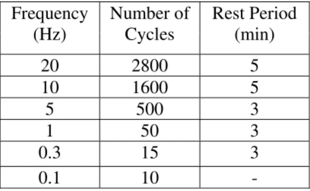
The main features of the test protocol include loading frequencies, data acquisition, and rest periods (see Attachment 1). Tables 2 and 3 show the number of cycles and rest period durations associated with each frequency for testing at different temperatures.

Table 2: Test at temperature 40 and 30 oC Frequency (Hz) Number of Cycles Rest Period (sec.) 20 1000 5 10 700 5 5 250 3 1 15 2 0.3 10 2 0.1 5 -

Table 3: Test at temperature –10, 0 and 20 oC Frequency (Hz) Number of Cycles Rest Period (min) 20 2800 5 10 1600 5 5 500 3 1 50 3 0.3 15 3 0.1 10 -

The program also contains input options such as segment shape, frequency, number of cycles, control mode of the test, and deformation magnitude (see Attachment 2).

Moreover, a rest period between loading at a frequency and the other is important. This action enables the machine to release the force applied during a frequency beforeproceeding to the next (see Table 2, Table 3, and Attachments 1 and 4).

9.4 Data Acquisition System: The data acquisition system shall have enough channels to enable

automatic collection of data including real time, applied strain as measured by the two extensometers and the resulting force detected by the load cell at a sampling rate of 100 points

(12)

FILE PATH:

PAGE 10 OF 22

per cycle. Data shall be collected during the last 50 cycles. A circular buffer type with a size of 5000 points represents a good selection to collect the last 50 cycles (see Attachment 5).

10. TEST PROCEDURE

The recommended test series consists of five test temperatures {(-10, 0, 20, 30, and 40 °C) (14, 32, 68, 86 and 104°F)} and six loading frequencies (0.1, 0.3, 1.0, 5, 10, and 20 Hz). Each specimen should be tested for the 30 combinations of temperature and frequency, starting with the lowest temperature and proceeding to the highest. Testing at a given temperature should begin with the highest frequency of loading and proceed to the lowest. The following sub-paragraphs explain the step-by-step test procedure.

10.1 Place the lower adaptor on top of the load cell, and firmly connect them together.

10.2 Place the prepared specimen inside the thermal chamber. Connect the lower adaptor to the lower hardened steel disc already glued to the specimen.

10.3 Connect the upper adaptor to the upper hardened steel disc already glued to the specimen. 10.4 Set the temperature of the thermal chamber to the specified test temperature.

Note 2: A temperature equilibrium test is recommended using a specimen with a thermocouple mounted at the centre to determine the time required by the specimen to reach the specified test temperature. However, a minimum of one and a half hour was found to achieve equilibrium at the desired temperature.

10.5 At the end of sample conditioning, intended to reach temperature equilibrium, bring the loading actuator in contact with the upper adaptor and connect them firmly. Make sure they are well centered to avoid eccentricity of the load. Apply a small contact load (up to 5% of the maximum force expected at the specified temperature) to avoid the effect of an impact load on the specimen.

10.6 Adjust and balance the electronic measuring system as necessary.

10.7 Apply a sinusoidal displacement corresponding to 120 microstrain by automatically initiating the computerized test protocol mentioned in section 9.3.

(13)

FILE PATH:

PAGE 11 OF 22

10.8 During the test, monitor axial displacement and resulting force on the screen. Make sure that the signals for applied displacement and corresponding force conform to the input cyclic waveforms. Adjust the recorder chart speed such that at least 3 complete cycles are displayed.

11. TEST OUTPUT AND DATA PROCESSING

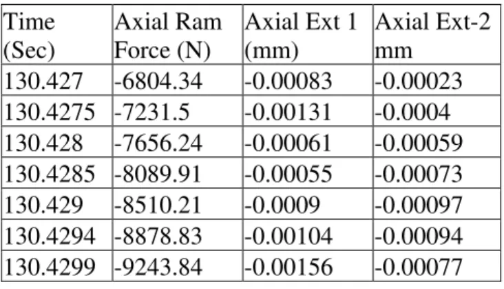
11.1 Output: The data acquisition system collects data automatically at real time (sec) for applied strain as measured by the two extensometers and the resulting force detected by the load cell. Typical data collected is shown in Table 4.

Table 4: Typical data acquired Time (Sec) Axial Ram Force (N) Axial Ext 1 (mm) Axial Ext-2 mm 130.427 -6804.34 -0.00083 -0.00023 130.4275 -7231.5 -0.00131 -0.0004 130.428 -7656.24 -0.00061 -0.00059 130.4285 -8089.91 -0.00055 -0.00073 130.429 -8510.21 -0.0009 -0.00097 130.4294 -8878.83 -0.00104 -0.00094 130.4299 -9243.84 -0.00156 -0.00077

11.2 Processing: The acquired data, similar to that shown in Table 4 should be processed to calculate stresses and strains for the last 3 cycles using Equation 1 and 2.

0 P =

A

σ --- (Equation 1)

Where A is the cross sectional area of specimen and P is the recorded axial force

0= L

(14)

FILE PATH:

PAGE 12 OF 22

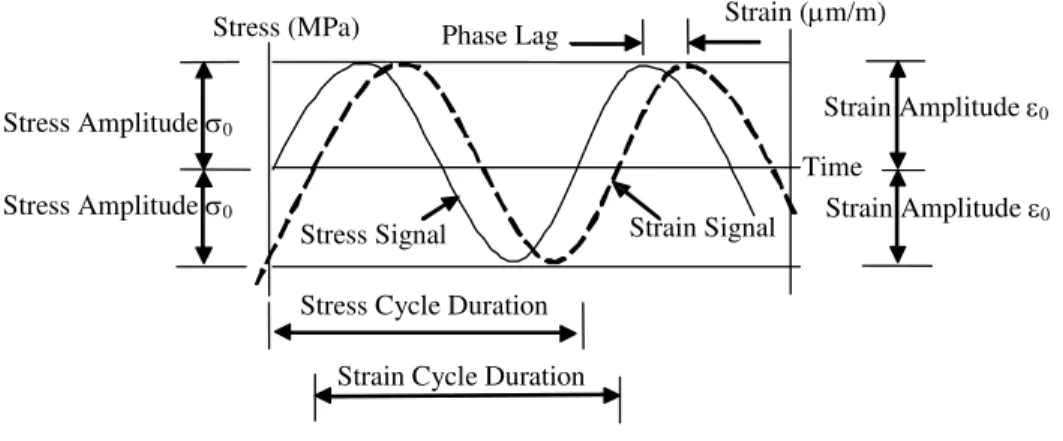
Where is the deformation measured by the controlled extensometer and L is the gauge length as shown in Figure 4. Δ

MTS

Gauge Length (L)

Figure 4: Axial extensometer model 632.11F-90

Stresses and strains are then plotted against time to determine stress (σo) and strain amplitudes

(εo)as shown in Figure 5.

Stress Amplitude σ0

Stress Signal Strain Signal Stress (MPa)

Stress Cycle Duration

Strain (μm/m)

Strain Cycle Duration Phase Lag

Time Stress Amplitude σ0

Strain Amplitude ε0

(15)

FILE PATH:

PAGE 13 OF 22

12. CALCULATIONS

Using the processed data:

12.1 Determine the average time ( ) lag between stress peak and strain peak values determined from Figure 5.

i

T

12.2 Calculate the phase angle as follows:

o p i T T 360 × = φ --- (Equation 3) Where: i

T = Time lag between the stress and strain cycles (sec)

p

T = Average time for a stress cycle (sec)

12.3 Calculate the dynamic modulus, E using the following equation: *

* 0

0

E σ

ε

= --- (Equation 4)

Parameters in Equation 4 as defined above (Section 11.2).

Note 3: – There are different methods for determining these parameters. These include peak search algorithms; curve fitting techniques, and Fourier Transform. However, curve-fitting techniques have a significant advantage over other methods in determining the amplitudes of stresses, strains and the phase angles. These parameters can be found easily using waveform equations that replace Equations 1, 2, and 3 as follows:

(16)

FILE PATH:

THIS DOCUMENT IS NOT CONTROLLED, UNLESS THE ABOVE QA SIGNATURE IS IN RED INK. PAGE 14 OF 22 1 sin( ) o a t σ = +σ ω ϕ+ --- (Equation 5) 2 sin( ) o b t ε = +ε ω ϕ+ --- (Equation 6) Where:

σand εare the stress and strain respectively at time t; σo and εo are the amplitude of stress and strain respectively;

ω = 2πf, the Angular velocity in radians, f is the frequency in Hz, a and b are regression constants; and

1, 2

ϕ ϕ Represent individual phase angles of stress and strain wave functions respectively.

The phase lag φ between stress and strain cycles is calculated as the difference of (ϕ ϕ₁− ₂) in radians

12.4 Calculate the storage modulus E1 as follows:

E1 = E cos * φ --- (Equation 7)

12.5 Calculate the loss modulus as follows:

E2 = E sin * φ --- (Equation 8)

13. RHEOLOGICAL MODEL

(17)

FILE PATH:

PAGE 15 OF 22

Results of the test (dynamic moduli and phase angles), calculated at a number of temperature and frequency combinations, may be fitted into a rheological model that enables the determination of the dynamic modulus at any given temperature and frequency.

The Huet-Sayegh model was adopted in this protocol as the rheological model used for characterizing asphalt materials. Figure 6 illustrates the model schematically and Equation (9) gives its analytical expression.

k E∞ – E₀ h E₀

σ

Figure 6: Schematic diagram of Huet-Sayegh model

( )

* 0 0 1 k E E E i E i i ω δ ωτ ωτ ∞ − − = + + + −h --- (Equation 9)

The model consists of eight parameters. Five of them are expressed explicitly in Equation 9, namely:

E0: is the high temperature stiffness;

(18)

FILE PATH:

PAGE 16 OF 22

δ, k, and h: are characteristics of the parabolic elements.

The other three parameters are determined implicitly using τ, which is referred to as the “Characteristics time” and it is calculated by the following equation:

( )

2

ln τ = +a bT+cT --- (Equation 10)

Where a, b, and c are regression constants representing material characteristics.

13.2 Determination of Huet-Sayegh model Parameters:

Dynamic moduli and phase angles, calculated at different temperatures and loading frequencies, are used to determine the eight parameters of the Huet-Sayegh rheological model. E0, E∞, δ, k,

and h are determined iteratively to achieve the best fit that can be obtained in the Cole-Cole and Black diagrams.

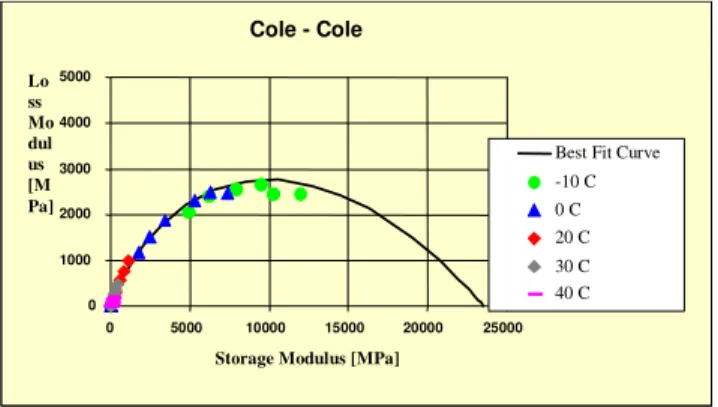
13.2.1 Cole-Cole Diagram:

The diagram is the result of plotting the storage modulus E1 versus the loss modulus E2. Figure 7

shows typical data plotted in cole-cole space.

Cole - Cole 0 1000 2000 3000 4000 5000 0 5000 10000 15000 20000 25000 Storage Modulus [MPa]

Lo ss Mo dul us [M Pa]

Best Fit Curve -10 C 0 C 20 C 30 C 40 C

(19)

FILE PATH:

PAGE 17 OF 22

13.2.2 Black Diagram:

This diagram illustrates the relationship between the dynamic modulus, E* versus the phase angle φ. Figure 8 shows typical data plotted in Black space.

igure 8: Typical Black diagram

3.2.3 Graphical Representation of Huet-Sayegh Model Parameters:

However, the regression

Black Diagram 0 10 20 30 40 50 60 10 100 1000 10000 100000

Log Complex Modulus [MPa] Ph ase An gle [de g]

Best Fit Curve -10 C 0 C 20 C 30 C 40 C F 1

E0, E∞, k, and h are illustrated graphically in Figures 9 and 10.

constants a, b, and c associated with the characteristics time τ are not expressed in either of the diagrams.

(20)

FILE PATH:

PAGE 18 OF 22

Storage Modulus [MPa]

E∞

Cole-

Cole Diagram

Loss Modulus [MPa]

t

an

-

1

(h

π/2)

tan -1(kπ/2)

E0

Figure 9:Graphical representation of Huet -Sayegh model parameters in Cole-Cole diagram

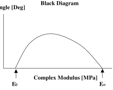
Phase Angle [Deg]

Complex Modulus [MPa]

Black Diagram

E∞

E0

(21)

FILE PATH:

PAGE 19 OF 22

Note 4: HUSAROAD program, a part of VEROAD Software developed by the “Netherlands

Pavement Consultants” is commercially available to assist in fitting laboratory data and

determining Huet-Sayegh model parameters.

14. REPORT

Report the test data including physical properties of the tested specimen and the 8 Huet-Sayegh model parameters as shown in Attachment 6.

Attachment 1: Main Window showing Multi-Purpose TestWare Program Created to Control the Test

(22)

FILE PATH:

PAGE 20 OF 22

ttachment 3: Typical Window Showing Signals of Data Recorded

Attachment 2: Window Showing Typical Command of Test Input at 20Hz Loading

(23)

FILE PATH:

PAGE 21 OF 22

Loading Attachment 4: Typical Window Showing Command of Rest Period After 20Hz

(24)

FILE PATH:

THIS DOCUMENT IS NOT CONTROLLED, UNLESS THE ABOVE QA SIGNATURE IS IN RED INK. PAGE 22 OF 22 1- Mix Identification: Mix Category: ____________________________________________________________ Local Classification: ________________________________________________________ Sample ID: _______________________________________________________________

2- Physical Properties of the Mix:

Nominal Maximum Aggregate Size mm (in): ____________________________________ Binder Type: ______________________________________________________________ Binder Content (%) _________________________________________________________

ir Voids Content (%): ______________________________________________________

- Huet-Sayegh Model Parameters:

me, τ, Coefficients

Attachment 6: Test Report Form

A

3

Model Coefficients Characteristic Ti Replicate

# E∞

(MPa)

E0