HAL Id: insu-02388761
https://hal-insu.archives-ouvertes.fr/insu-02388761
Submitted on 2 Dec 2019
least mean square algorithm
Mohamed Zaiani, Djelloul Djafer, Fatima Chouireb, Abdanour Irbah,
Mahfoud Hamidia
To cite this version:
Mohamed Zaiani, Djelloul Djafer, Fatima Chouireb, Abdanour Irbah, Mahfoud Hamidia. New method
for clear day selection based on normalized least mean square algorithm. Theoretical and Applied
Climatology, Springer Verlag, 2020, 139 (3-4), pp.1505-1512. �insu-02388761�
New Method for Clear Day Selection Based on Normalized Least
1
Mean Square Algorithm
2
Zaiani Mohamed1, Djafer Djelloul1, Chouireb Fatima2, Irbah Abdanour3 and Hamidia Mahfoud4
3
4
1Unité de Recherche Appliquée en Energies Renouvelables, URAER, Centre de Développement des Energies
5
Renouvelables, CDER, 47133, Ghardaïa, Algeria,
6
2Laboratoire des Télécommunications, Signaux et Systèmes LTSS, Université Amar Telidji de Laghouat, Algeria,
7
3Laboratoire Atmosphères, Milieux, Observations Spatiales (LATMOS), CNRS : UMR8190, Université Paris VI
-8
Pierre et Marie Curie, Université de Versailles Saint-Quentin-en-Yvelines, INSU, 78280, Guyancourt, France,
9
4USTHB, Faculty of Electronics and Computer Science, LCPTS, Speech Communication and Signal Processing
10
Laboratory, P.O Box32, Bab Ezzouar, Algiers 16 111, Algeria,
11
Corresponding author: [email protected], +213 (0) 663153531
12
Abstract. A new method is proposed to select clear days from data sets of solar irradiation recorded with
ground-13
based instruments. The knowledge of clear days for a given site is of prime importance both for the study of
14
turbidity and for the validation of empirical models of Global Solar Radiation (GSR). Our innovative method is
15
based on the Normalized Least Mean Square (NLMS) algorithm that estimates noise according to a GSR model. The
16
developed method named Clear Day Selection Method (CDSM) is compared to the well-known clearness index
17
criteria (kt) taking data collected at Tamanrasset in Algeria during the period 2005-2009. The root mean square error
18
(rmse), the mean absolute percentage error (mape) and the dependence of model error (mbe) are considered for the
19
comparison. A different number of clear days is found with both methods, with additionally a kt dependency for the
20
clearness index criteria. The average values of rmse, mape and mbe between the daily average of the measured GSR
21
and its estimate using a model are better in case of CDSM for the period 2005-2009. Indeed, we found 25.28 W/m2,
22
4.61 % and 2.09 W/m2 respectively for CDSM and 42.48 W/m2, 7.63 % and -5.91 W/m2 for the clearness index
23
method with kt = 0.7. We also found that GSR of clear days is well correlated with the model in case of CDSM,
24
which gives good confidence in our results.
25
Keywords clearness index, NLMS, adaptive algorithm, solar radiation
26
1 2 3 4 5 6 7 8 9 10 11 12 13 14 15 16 17 18 19 20 21 22 23 24 25 26 27 28 29 30 31 32 33 34 35 36 37 38 39 40 41 42 43 44 45 46 47 48 49 50 51 52 53 54 55 56 57 58 591- Introduction
27
The Global Solar Radiation (GSR) is the total amount of solar radiation received by the Earth surface and
28
corresponds to the contribution of direct, diffuse and reflected solar radiation. Direct solar radiation is the
29
propagation of the beam directly through the atmosphere to the surface of the Earth, while diffuse solar radiation is
30
scattered in the atmosphere. Solar radiation is affected during its propagation through the atmosphere by atoms and
31
molecules (ozone, water vapor, carbon dioxide ...) as well as by liquid and solid aerosols dispersed or grouped in
32
clouds (Kaskaoutis 2008). Solar radiation measurements on the ground then depend on the site location. The
33
location must indeed be taken into account when we are interested in the quality and amount of solar radiation. GSR
34
is one of the most important parameters in solar energy designs and/or applications (Badescu et al. 2013; Reno et al.
35
2012). Analyzing solar radiation properties in a given location requires long-term data and both use of empirical,
36
semi-empirical or physical models and specific techniques such as neural networks (Senkal 2015; Mohandes 2012).
37
Many studies were carried out to estimate and/or predict solar radiation using available meteorological (air
38
temperature, relative humidity ...) and geographical (sunshine hours, latitude ...) parameters (Wong and Chow 2001;
39
Victor et al. 2016; Gueymard 2012). These models are needed to obtain the correct designs and outputs of solar
40
power plants in case of clear sky conditions. Selecting clear days from recorded datasets is the first step in modelling
41
solar radiation under these conditions. The clearness index method, based essentially on the calculation of a
42
parameter related to measured solar radiation, is widely used for this purpose (Alves et al. 2013; Khem et al.
43
2012; Mellit et al. 2008). Authors then sorted day types using the parameter according to their own criteria. The
44
sky is, for some, clear when its value is between 0.65 and 1, partly cloudy when and cloudy if
45
(Gueymard 2012; Alves et al. 2013). For other authors, a clear sky is when (Bendt et al.
46
1981; Ahmed et al. 2008), higher than 0.6 (Reindl et al. 1990) or 0.7 (Li and Lam 2001; Li et al. 2004). Iqbal
47
considers that the sky is clear when is between 0.7 and 0.9 (Iqbal 1983). also varies in time (Serban 2009) and
48
depends on regions. Its value in most tropical regions is between and for a clear sky (Ndilemeni et al.
49
2013). We see clearly with this short bibliographic that there is a great disparity in the definition of a clear sky using
50
this parameter and there is no clear method for its estimation. The choice of its value can be crucial to distinguish
51
clear days from turbid ones. A wrong choice will affect mainly the number of clear and turbid days in a dataset
52
4 5 6 7 8 9 10 11 12 13 14 15 16 17 18 19 20 21 22 23 24 25 26 27 28 29 30 31 32 33 34 35 36 37 38 39 40 41 42 43 44 45 46 47 48 49 50 51 52 53 54 55 56 57the issue of the clearness index choice led us to develop a new method for classifying clear and turbid days. The
54
method is based on the Normalized Least Mean Square algorithm (Sharma and Mehra 2016; Dixit and Nagaria
55
2017), which is an adaptive algorithm based on minimization of the norm of differences between estimate and real
56
signal. This method is often used in signal processing for noise identification or cancellation (Sahu and Sinha 2015;
57
Gupta and Bansal 2016) and is therefore suited for GSR measurements. Indeed, its perturbations are due to solar
58
radiation propagation through the atmosphere and are well assimilated as noise in our process. In this work, we first
59
present the clearness index algorithm used to distinguish clear and turbid days, and then introduce CDSM, the
60
NLMS method for Clear Days Selection. A comparison of these methods will then be made and the results
61
discussed.
62
2- The Clearness index method
63
The clearness index was introduced by Liu and Jordan to quantify stochastic property conditions for a given site
64
(Liu and Jordan 1960). Interval values for are taken to separate clear and turbid days but are often site dependent
65
(see Section 1), which leads to misinterpretation of the results, especially when authors compare and study empirical
66
models. The clearness index is defined over time as the ratio between the terrestrial global solar radiation
67
on a horizontal surface and the extraterrestrial one :
68
(1)
69
where in / is given by:
70
(2)
71
is the Total Solar Irradiance (TSI) equal to 1361 / (Myhre et al. 2013) and N the day number in the year
72
(N=1 is the first day in the year and N=365 the last one). , and are respectively the latitude of the location, the
73
solar declination angle and the hour angle at sunrise in degrees.
74
An algorithm based on the instantaneous clearness index was first developed for our work to automatically select
75
days from a huge dataset. The main steps of the algorithm are:
76
Selection of records of a given day where the Sun elevation is higher than 10°.
77
4 5 6 7 8 9 10 11 12 13 14 15 16 17 18 19 20 21 22 23 24 25 26 27 28 29 30 31 32 33 34 35 36 37 38 39 40 41 42 43 44 45 46 47 48 49 50 51 52 53 54 55 56 57 58 59This condition is only intended to prevent the presence of haze early in the morning or late in the afternoon.
78
This could lead to considering a clear day as not being one.
79
Calculation of the extraterrestrial solar radiation for the same day.
80
Calculation of the instantaneous clearness index between sunrise and sunset using Equation 1.
81
3- Normalized Least Mean Square Method for Clear Days Selection
82
We present in this section the Normalized Least Mean Square (NLMS) algorithm and then how we use it to select
83
clear days from data sets.
84
3-1. The NLMS algorithm
85
The Least Mean Square (LMS) algorithm was first developed by Widrow and Hoff in 1959 for speech recognition
86
applications. It is today one of the most widely used algorithms in adaptive filtering mainly due to its efficiency and
87
computational simplicity. LMS algorithms are a class of adaptive filters used to generate a desired filter that
88
produces least mean squares of the error signal i.e. difference between desired and real signal. The algorithm starts
89
by assuming small weights (zero in most cases) at each step and finding the gradient of the estimated error. Weights
90
are then updated according to the following equation (Dixit and Nagaria 2017):
91
92
Here is an input vector with delayed values in time. w(n) = [w0(n) w1(n) w2(n) … wL-1 (n)]T is a vector with
93
components containing the tap weight coefficients of the adaptive FIR (Finite Impulse Response) filter at time ,
94
is the estimated filter error at and the subscript stands for transpose operator. The parameter is known as
95
the step size parameter and is a small positive constant. This parameter controls the influence of the updating factor.
96
Selection of a suitable value of is imperative for the performance of the LMS algorithm. The time taken by the
97
adaptive filter to converge into the optimal solution will be too long if its value is too small. The adaptive filter
98
becomes unstable if is too large and its output diverges (Sharma and Mehra 2016; Dixit and Nagaria 2017). The
99
stability condition of the LMS algorithm is / , where is is the largest eigenvalue of the
100
autocorrelation matrix of the input signal . The main disadvantage of LMS algorithm is the fixed step size
101
4 5 6 7 8 9 10 11 12 13 14 15 16 17 18 19 20 21 22 23 24 25 26 27 28 29 30 31 32 33 34 35 36 37 38 39 40 41 42 43 44 45 46 47 48 49 50 51 52 53 54 55 56 57parameter for every iteration. This requires knowledge of the input signal statistics prior to starting the adaptive
102
filtering operation. The NLMS algorithm is an extension of the LMS one, which by passes this issue by calculating
103
the maximum step size value. This step size is proportional to the inverse of the total expected energy of
104
instantaneous coefficients of the input vector . The recursion formula for NLMS algorithm is given by
105
(Hamidia and Amrouche 2016):
106
(4)
107
where is the adaptation step size of NLMS and is a regularization constant used to avoid division
108
by zero.
109
The NLMS algorithm is implemented according to the following steps:
110
The output signal of the adaptive filter is calculated by:
111
(5)
112
The estimated filter error signal at step (n) is computed as the difference between the desired signal and
113
the filter output:
114
(6)
115
The filter tap weights are updated in preparation for the next iteration using Equation 4.
116
Figure 1. Adaptive filtering
Basic modules of an adaptive filter are shown in Figure 1 (Dixit and Nagaria 2017). The output of the adaptive filter
117
and the desired response are processed to assess its quality with respect to requirements of a particular application.
118
This module generates the filter output using input signal measurements. The filtering structure is linear or nonlinear
119
according to the designer and its parameters are adjusted by the adaptive algorithm.
120
4 5 6 7 8 9 10 11 12 13 14 15 16 17 18 19 20 21 22 23 24 25 26 27 28 29 30 31 32 33 34 35 36 37 38 39 40 41 42 43 44 45 46 47 48 49 50 51 52 53 54 55 56 57 58 59Figure 2. Flowchart of CDSM
3-2. The CDSM algorithm
121
Our proposed method for selecting clear days present in dataset is based on the NLMS algorithm and any parametric
122
GSR model. The Capderou model has been used in this work (Capderou 1987). This parametric model uses the
123
Linke turbidity to compute the global, direct and diffuse components of clear sky solar radiation. The main idea of
124
the method is to compare estimated GSR with measurements i.e. GSR resulting from adaptive filtering when taking
125
GSR measurements as input are compared to GSR model of clear sky. CDSM is summarized by the following steps
126
(Figure 2) (Quadri et al. 2017):
127
128
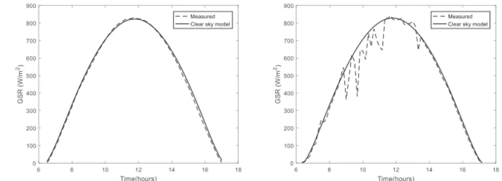
Figure 3. Examples of daily recorded GSR (dashed line) superposed to the clear sky model (full line).
Each daily GSR is fitted with a clear sky GSR model.
129
The measured GSR is subjected to a parameterized FIR filtering with coefficients (see previous section):
130
4 5 6 7 8 9 10 11 12 13 14 15 16 17 18 19 20 21 22 23 24 25 26 27 28 29 30 31 32 33 34 35 36 37 38 39 40 41 42 43 44 45 46 47 48 49 50 51 52 53 54 55 56 57a sample of the modeled GSR is obtained.
131
The estimated filter errorbetween samples of modelled GSR and clear sky GSR model is calculated.
132
The obtained estimated filter error is used to calculate the next step that is used to readjust FIR filter
133
coefficients ( )
134
Steps 1-4 are considered for all samples of the measured GSR
135
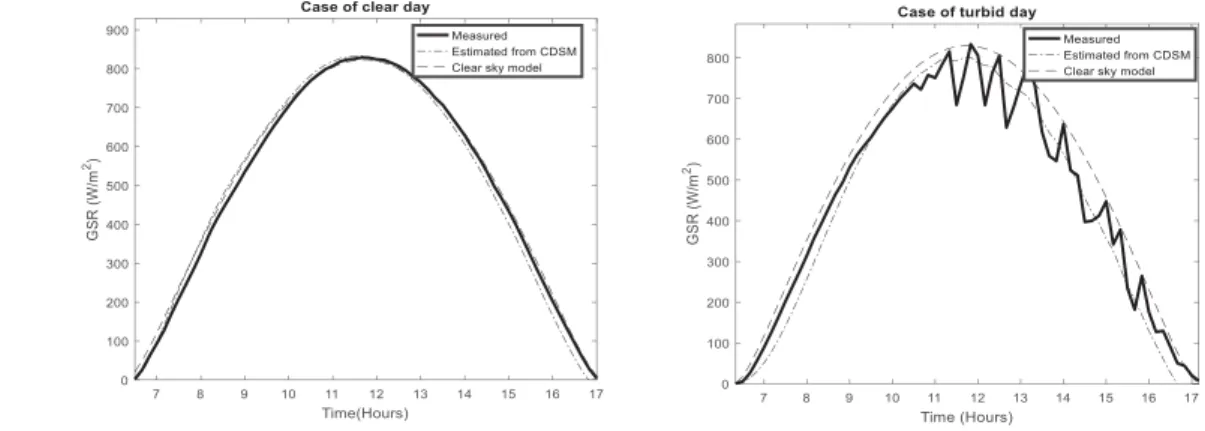
Figure 4. CDSM behavior in case of a clear (left) and a turbid day (right).
Figure 3 plots an example of daily measured GSR (dashed line) superposed to the clear sky GSR model (full line)
136
for both clear (left plot) and turbid (right plot) days. Figure 4 shows CDSM behavior to estimate GSR in case of
137
clear (left plot) and turbid days (right plot). The adaptive filter takes a measured GSR as input and produces a
138
modeled GSR by recursively adjusting the filter parameters to handle the disturbances present in the GSR
139
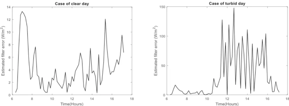
measurement. Figure 5 plots the estimated filter error obtained when CDSM is run on data of Figure 4. We see that
140
the method allows having a modelled GSR more or less disturbed according to the data considered. It will be close
141
to the GSR model when the estimated filter error is small i.e. the case of clear days. We will consider in our study
142
that clear days correspond to the estimated filter error less than 20 / ; otherwise they are considered as turbid.
143
4 5 6 7 8 9 10 11 12 13 14 15 16 17 18 19 20 21 22 23 24 25 26 27 28 29 30 31 32 33 34 35 36 37 38 39 40 41 42 43 44 45 46 47 48 49 50 51 52 53 54 55 56 57 58 59Figure 5. Estimated filter error of the GSR estimate for a clear (left) and a turbid day (right).
4- Comparison of clear day selection methods. Results and discussion.
144
We use GSR data recorded from 2005 to 2009 in southern Algeria to compare the efficiency of CDSM relative to
145
other methods. Let us first present the data set.
146
4-1. Data set of solar radiation
147
Data used in this work were collected at the Regional Meteorological Center (Direction Météo Régional Sud, Office
148
National de la Météorologie, Algeria) at Tamanrasset (22.79°N, 5.53°E, 1377 m a.s.l.) in southern Algeria between
149
2005 and 2009. Instruments and methods for data collection are the same as those described in detail by Djafer and
150
Irbah (Djafer and Irbah 2013). The main difference is that the three components of solar radiation are recorded every
151
minute at Tamanrasset together with temperature, humidity and pressure. Instruments that measure direct, global and
152
diffuse solar radiation components are EKO type instruments (http://eko-eu.com/) (see Figure 6). They are cleaned
153
two to three times a week depending on weather conditions and calibrated every three years. Data were calibrated
154
with the TSI of 1367 / since it was the current value at this period (2005 - 2009). A correction factor is applied
155
to the data since the TSI of 1361 / is now adopted. This factor is the ratio between current and previous TSI.
156
4 5 6 7 8 9 10 11 12 13 14 15 16 17 18 19 20 21 22 23 24 25 26 27 28 29 30 31 32 33 34 35 36 37 38 39 40 41 42 43 44 45 46 47 48 49 50 51 52 53 54 55 56 57Figure 6. Radiometric station for measuring global, direct and diffuse solar radiation: (1) Pyranometer for measuring the global solar irradiance. (2) Pyranometer for measuring the diffuse. (3) Pyrheliometer for measuring the direct solar irradiance, (4) Shaded pyranometer. (5) The 2-axis solar tracker.
4-2. Results and discussion
157
We used the five years of GSR measurements (see section 4.1) and determined clear days present in the data set with
158
the clearness index, wavelet based method (Djafer et al. 2017) and CDSM. Results are given in Table 1 and plotted
159
in Figure 7 where error bars are one standard deviation. values widely used in the literature to select clear days
160
were considered for the comparison, that is .
161
Table 1. Number of clear days per year selected with different methods Years 2005 2006 2007 2008 2009 Wavelet method 59 30 65 98 24 CDSM 136 133 173 173 120 =0.5 303 316 319 322 305 =0.6 244 254 279 274 254 =0.7 114 133 158 170 139 =0.8 2 7 6 14 7 4 5 6 7 8 9 10 11 12 13 14 15 16 17 18 19 20 21 22 23 24 25 26 27 28 29 30 31 32 33 34 35 36 37 38 39 40 41 42 43 44 45 46 47 48 49 50 51 52 53 54 55 56 57 58 59
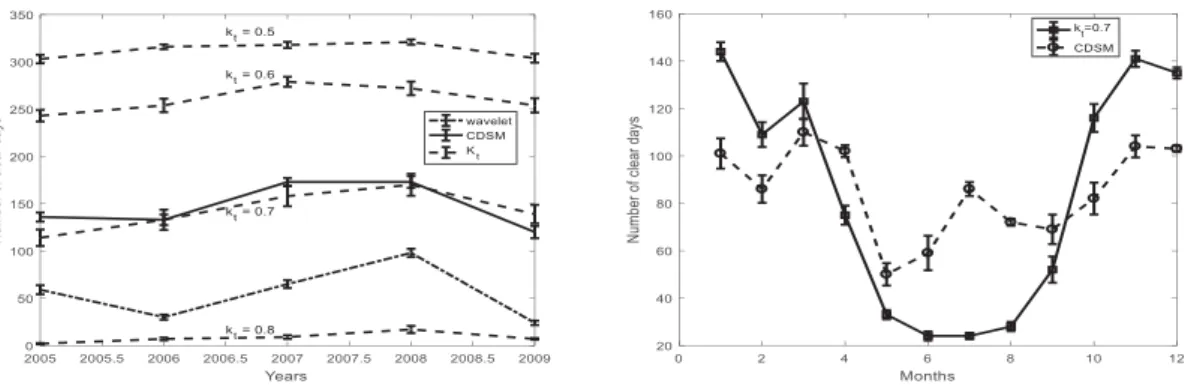
Figure 7. Number of clear days selected with the different methods: number per year (left) and per month (right).
We observe in the left plot of Figure 7 that the number of clear days per year obtained with CDSM is close to what is
162
found with . Lower values overestimate the number of clear days while higher ones underestimate it. The
163
wavelet method seems to underestimates the yearly number of clear days due to excessive constraints on GSR
164
disturbances when setting the selection threshold. The three methods show the same trend of the yearly number of
165
clear days with a maximum around 2008. If we look at the monthly values of clear days computed over the period
166
2005-2009, we observe a difference between CDSM results and those obtained with the clearness index with
167
(see right plot of Figure 7). Curves have similar shapes but the number range for the clearness method is large
168
relative to the CDSM one. There is quasi no clear days found for months between May and August with
169
leading to suppose that its value needs to be adjusted during processing as reported in section 1. We note that the
170
number of clear days at Tamanrasset is lower during the months of May and September-October compared to the
171
others.
172
Finally, we compared GSR of clear days obtained with both and CDSM to those estimated by the model
173
described in Zaiani et al. (2017). This parametric model used Artificial Neural Network to estimate GSR of a given
174
clear day. We used several parameters to quantify the comparison among which are the root mean square error
175
(rmse), the normalized root mean square error (nrmse), the mean absolute percentage error (mape), the dependence
176
of model error (mbe) and the normalized dependence of model error (nmbe). Comparison results are given in Table
177
2. We note that the model fits better the measured GSR of clear days determined with CDSM. Indeed, we have a
178
mean of 0.97, an rmse of 25.28 / , an mbe of 2.09 / and a mape of 4.16 % while we have a mean of
179
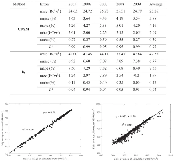
4 5 6 7 8 9 10 11 12 13 14 15 16 17 18 19 20 21 22 23 24 25 26 27 28 29 30 31 32 33 34 35 36 37 38 39 40 41 42 43 44 45 46 47 48 49 50 51 52 53 54 55 56 570.94, an rmse of 42.58 / , an mbe of 1.97 / and a mape of 7.55 % for the clearness index method. Figure 8
180
plots the correlation between daily average measured GSR of clear days selected with CDSM (left plot) and with the
181
clearness index method ( ) (right plot) versus daily average calculated GSR. We note that GSR of clear days
182
selected with CDSM are very well correlated with the model compared to what we obtain with the clearness index
183
method. The correlation factor is 0.99 for CDSM and 0.95 using criteria. We may conclude when looking at this
184
plot that we can be confident in the results obtained from CDSM.
185
Table 2. Annual average errors between measured and calculated GSR
186
Method Errors 2005 2006 2007 2008 2009 Average
CDSM rmse ( / ) 24.63 24.72 26.75 25.51 24.79 25.28 nrmse (%) 3.63 3.64 4.43 4.19 3.54 3.88 mape (%) 4.26 4.27 5.33 5.01 4.20 4.16 mbe ( / ) 2.01 2.00 2.25 2.15 2.05 2.09 nmbe (%) 0.27 0.27 0.59 0.55 0.27 0.39 0.99 0.99 0.95 0.95 0.99 0.97 kt rmse ( / ) 42.00 41.45 44.11 37.47 47.84 42.58 nrmse (%) 6.92 6.60 7.07 5.89 7.38 6.77 mape (%) 7.56 7.29 7.82 6.68 8.40 7.55 mbe ( / ) 1.24 2.97 2.89 2.54 -0.2 1.97 nmbe (%) 0.11 0.43 0.40 0.35 0.03 0.27 0.94 0.94 0.94 0.95 0.93 0.94
Figure 8. Correlation between daily average of calculated and measured GSR obtained with CDSM (left) and with
187
the clearness index with .
188
4 5 6 7 8 9 10 11 12 13 14 15 16 17 18 19 20 21 22 23 24 25 26 27 28 29 30 31 32 33 34 35 36 37 38 39 40 41 42 43 44 45 46 47 48 49 50 51 52 53 54 55 56 57 58 595- Conclusion
189
A new method to select clear days in data sets of solar radiation is presented in this work. This method we denoted
190
CDSM, is based on NLMS algorithm. We first compared CDSM to the clearness index method taking the most used
191
value and found that our method gives a higher number of clear days when using the same data set. We
192
took a data set of 5 years of solar radiation measurements collected at the Tamanrasset ONM. We then validated
193
CDSM using the clear days selected by both methods to model daily GSR. The analysis of the difference between
194
GSR of the clear days selected with CDSM and calculated for these days with the model shows a very good
195
agreement. We found that yearly values vary between (i) 4.20 and 5.33 % for mape, (ii) 0.95 and 0.99 for , (iii)
196
24.63 and 26.75 / for rmse and (iv) 2.00 and 2.25 / for mbe. Finally, we performed a comparison of daily
197
average GSR of clear days obtained with both CDSM and the clearness index method with and those
198
estimated with the model. We found that the GSR of clear days selected with CDSM are better correlated with the
199
model than those obtained with the clearness index method. The correlation coefficient is 0.99 for CDSM and 0.95
200
using criteria. We can emphasize that our method was developed using daily measured GSR but may also be
201
adapted to detect clear and turbid short periods in measurements. These short periods are very useful for studying
202
the environment and regional frequency of clouds. In addition, knowledge of the occurrence of clear days on a site
203
also has many other interests. This is particularly the case before any photovoltaic or thermal installation for which
204
solar radiometric measurements over a longer or shorter period are necessary. Our work is then very useful to give
205
the relevant information on the number of clear days for a given site and consequently to predict the energy that
206
these facilities will produce in this region.
207
References
208
Ahmed MA, Ahmad F, Akhtar MW (2008) Estimation of Global and Diffuse Solar Radiation for Hyderabad, Sindh,
209
Pakistan. Journal of Basic and Applied Sciences 5: 73-77
210
Alves MdC, Sanches L, Nogueira JDS, Silva VAM (2013) Effects of Sky Conditions Measured by the Clearness
211
Index on the Estimation of Solar Radiation Using a Digital Elevation Model. Atmospheric and Climate
212
Sciences 3: 618-626213
4 5 6 7 8 9 10 11 12 13 14 15 16 17 18 19 20 21 22 23 24 25 26 27 28 29 30 31 32 33 34 35 36 37 38 39 40 41 42 43 44 45 46 47 48 49 50 51 52 53 54 55 56 57Badescu V, and Gueymard CA, Cheval S, Oprea C, Baciu M, Dumitrescu A, Iacobescu F, Milos I, Rada C (2013)
214
Accuracy analysis for fifty-four clear-sky solar radiation models using routine hourly global irradiance
215
measurements in Romania. Renewable Energy 55: 85-103
216
Bendt P, Collares-Pereira M, Rabl A (1981) The frequency distribution of daily insolation values. Solar Energy 27:
217
1-5
218
Capderou M (1987) Modèles Théoriques et Expérimentaux. Atlas Solaire de l’Algérie, Tome 1, Vol. 1 et 2, Office
219
des Publications Universitaires, Algérie
220
Dixit S, Nagaria D (2017) LMS Adaptive Filters for Noise Cancellation: A Review. International Journal of
221
Electrical and Computer Engineering (IJECE) 7: 2520 2529
222
Djafer D, Irbah A (2013) Estimation of atmospheric turbidity over Ghardaia city. Atmospheric Research 128: 78-84
223
Djafer D, Irbah A, Zaiani M (2017) Identification of clear days from solar irradiance observations using a new
224
method based on the wavelet transform. Renewable Energy 101: 347- 355
225
Gueymard CA (2012) Clear-sky irradiance predictions for solar resource mapping and large-scale applications:
226
Improved validation methodology and detailed performance analysis of 18 broadband radiative models.
227
Solar Energy 86: 2145-2169
228
Gupta N, Bansal P (2016) Evaluation of Noise Cancellation Using LMS and NLMS Algorithm. International Journal
229
of Scientific & Technology Research 5: 69-72
230
Hadei SA, lotfizad M (2010) A Family of Adaptive Filter Algorithms in Noise Cancellation for Speech
231
Enhancement. International Journal of Computer and Electrical Engineering, Vol. 2, No. 2
232
Hamidia M, Amrouche A (2016) Improved variable step-size NLMS adaptive filtering algorithm for acoustic echo
233
cancellation. Digital Signal Processing 49: 44-55
234
Iqbal M (1983) An Introduction to Solar Radiation. Academic Press, Toronto
235
Kaskaoutis DG, Kambezidis HD (2008) Comparison of the Angstrom parameters retrieval in different spectral
236
ranges with the use of different techniques. Meteorol Atmos Phys 99: 233–246
237
Khem NP, Binod KB, Balkrishna S, Berit K (2012) Estimation of Global Solar Radiation Using Clearness Index and
238
4 5 6 7 8 9 10 11 12 13 14 15 16 17 18 19 20 21 22 23 24 25 26 27 28 29 30 31 32 33 34 35 36 37 38 39 40 41 42 43 44 45 46 47 48 49 50 51 52 53 54 55 56 57 58 59Cloud Transmittance Factor at Trans-Himalayan Region in Nepal. Energy and Power Engineering 4:
415-239
421
240
Li DHW, Lam JC (2001) An analysis of climate parameters and sky condition classifications. Building and
241
Environment 36: 435-445
242
Li DHW, Lau CCS, Lam JC (2004) Overcat sky conditions and luminance distribution in Hong Kong. Building and
243
Environment 39: 101-108
244
Liu BYH, Jordan RC (1960) The interrelationship and characteristic distribution of direct, diffuse and total solar
245
radiation. Solar Energy 4: 1-19
246
Mellit A, Kalogirou SA, Shaari S, Salhi H, Hadj Arab A (2008) Methodology for predicting sequences of mean
247
monthly clearness index and daily solar radiation data in remote areas: Application for sizing a stand-alone
248
PV system. Renewable Energy 33: 1570-1590
249
Mohandes MA (2012) Modeling global solar radiation using Particle Swarm Optimization (PSO). Solar Energy 86:
250
3137-3145
251
Myhre G, Shindell D, Bréon FM, Collins W, Fuglestvedt J, Huang J, Koch D, Lamarque JF, Lee D, Mendoza B,
252
Nakajima T, Robock A, Stephens G, Takemura T and Zhang H (2013) Anthropogenic and Natural Radiative
253
Forcing. In: Climate Change 2013: The Physical Science Basis. Contribution of Working Group I to the
254
Fifth Assessment Report of the Intergovernmental Panel on Climate Change.
255
Ndilemeni CC, Momoh M, Akande JO (2013) Evaluation of clearness index of Sokoto Using Estimated Global
256
Solar Radiation. Journal of Environmental Science, Toxicology and Food Technology 5: 51-54
257
Okogbue EC, Adedokunb JA, Holmgrenc B (2009) Review Hourly and daily clearness index and diffuse fraction at
258
a tropical station, Ile-Ife, Nigeria. International Journal of Climatology 29: 1035-1047
259
Quadri A, Manesh MR, Kaabouch N (2017) Noise Cancellation in Cognitive Radio Systems: A Performance
260
Comparison of Evolutionary Algorithms. IEEE 7th Annual Computing and Communication Workshop and
261
Conference (CCWC)
262
Radhika C, Ramkiran DS, Khan H, Usha M, Madhav BTP, Srinivas PK, Ganesh GV (2011) Adaptive Algorithms for
263
4 5 6 7 8 9 10 11 12 13 14 15 16 17 18 19 20 21 22 23 24 25 26 27 28 29 30 31 32 33 34 35 36 37 38 39 40 41 42 43 44 45 46 47 48 49 50 51 52 53 54 55 56 57Acoustic Echo Cancellation in Speech Processing. Ijrras 7 :38-42
264
Reindl DT, Beckman WA, Duffie JA (1990) Diffuse fraction correlation. Solar Energy 45: 1-7
265
Reno MJ, Hansen CW, Stein JS (2012) Global Horizontal Irradiance Clear Sky Models: Implementation and
266
Analysis. Sandia National Laboratories SAND2012-2389
267
Sahu K, Sinha R (2015) Normalized Least Mean Square (Nlms) Adaptive Filter for Noise Cancellation. International
268
Journal of Proresses in Engineering, Management, Science and Humanities 1: 49-53
269
Senkal O (2015) Solar radiation and precipitable water modeling for Turkey using artificial neural networks.
270
Meteorol Atmos Phys. DOI 10.1007/s00703-015-0372-6
271
Serban C (2009) Estimating Clear Sky Solar Global Radiation Using Clearness Index, for Brasov Urban Area.
272
International Conference on Maritime and Naval Science and Engineering, ISSN: 1792-4707
273
Sharma L, Mehra R (2016) Adaptive Noise Cancellation using Modified Normalized Least Mean Square Algorithm.
274
International Journal of Engineering Trends and Technology (IJETT) 34: 215-219
275
Victor HQ, Almorox J, Mirzakhayot I, Saito L (2016) Empirical models for estimating daily global solar radiation in
276
Yucatán Peninsula, Mexico. Energy Conversion and Management 110: 448-456
277
Wong LT, Chow WK (2001) Solar radiation model. Applied Energy 69: 191-224
278
Zaiani M, Djafer D, Chouireb F (2017) New Approach to Establish a Clear Sky Global Solar Irradiance Model.
279
International Journal of Renewable Energy Research 7: 1454-1462