Bouncing and Walking Droplets:
Towards a Hydrodynamic Pilot-Wave Theory
by
ARCHNiE
MASSACHUSETTS INSTMr E
Jan Molacek
OF TECHNOLOGYB.A., Mathematics, University of Cambridge (2007)
JUL 2 5 2013
Submitted to the Department of Mathematics
LIBRARIES
in partial fulfillment of the requirements for the degree of
Doctor of Philosophy
at the
MASSACHUSETTS INSTITUTE OF TECHNOLOGY
June 2013
@
Jan Molakek, MMXIII. All rights reserved.
The author hereby grants to MIT permission to reproduce and to
distribute publicly paper and electronic copies of this thesis document
in whole or in part in any medium now known or hereafter created.
Author ...
Department of Mathematics
.ay
3, 2013
Certified by...
...
-......
.-John W. M. Bush
Professor of Applied Mathematics
Thesis Supervisor
Accepted by ...
Michel Goemans
Bouncing and Walking Droplets:
Towards a Hydrodynamic Pilot-Wave Theory
by
Jan Mola6ek
Submitted to the Department of Mathematics on May 3, 2013, in partial fulfillment of the
requirements for the degree of Doctor of Philosophy
Abstract
Coalescence of a liquid drop with a liquid bath can be prevented by vibration of the bath. In a certain parameter regime, a purely vertical bouncing motion may ensue. In another, this bouncing state is destabilized by the droplet's wavefield, leading to drop motion with a horizontal component called walking. The walking drops are of particular scientific interest because Couder and coworkers have demonstrated that they exhibit many phenomena reminiscent of microscopic quantum particles. Nevertheless, prior to this work, no quantitative theoretical model had been developed to rationalize and inform the experiments before our work.
In this thesis, we develop a hierarchy of theoretical models of increasing com-plexity in order to describe the drop's vertical and horizontal motion in the relevant parameter range. Modeling the drop-bath interaction via a linear spring is found lacking; therefore, a logarithmic spring model is developed. We first introduce this model in the context of a drop impacting a rigid substrate, and demonstrate its accu-racy by comparison with existing numerical and experimental data. We then extend the model to the case of impact on a liquid substrate, and apply it to rationalize the dependence of the bouncing droplet's behaviour on the system parameters. The the-oretical developments have motivated further experiments, which have in turn lead to refinements of the theory.
We proceed by modeling the evolution of the standing waves created by impact on the bath, which enables us to predict the onset of walking and the dependence of the walking speed on the system parameters. New complex walking states are predicted,
and subsequently validated by our detailed experimental study. A trajectory equation for the horizontal motion is obtained by averaging over the vertical bouncing.
Thesis Supervisor: John W. M. Bush Title: Professor of Applied Mathematics
To my parents, Marie & Josef, in loving memory.
Acknowledgments
I would like to thank first of all my advisor John Bush, for his continued support, encouragement, patience and guidance, and for providing interesting problems to work on. I have learned a lot from him, from scientific writing to good eating, and I am very grateful for his hospitality.
The experimental data published in this thesis could not have been obtained without Daniel Harris, who built the set-up and taught me how to operate it. I am grateful to Anand Oza for valuable discussions and helpful comments, and to Oistein Wind-Willassen for his help with the experiments. I wish to thank also my thesis committee, Professors Ruben Rosales and Gareth McKinley.
On a more personal note, I would like to thank my family and friends in Boston, who helped me retain, at least partly, my sanity: Qinwen Xiao, Jonathan and Ying Rameseder, Hdskuldur Halldorsson, Anand Oza, Rosalie Belanger-Rioux, Tracy Washington, Eric Marberg, Mehdi Ben Abda, Alejandra Terminel, Alexandra van Geen and Renato Umeton. Special thanks go to Madeleine Patston for her patience and love, and for providing the light at the end of the tunnel.
Finally, I would like to mention my mathematics a physics teachers Iva Petrov4 and Premysl Sedivf, who encouraged me to pursue my scientific interests, and Viclav Cvitek, without whom I would not have considered studying outside of my native country.
Contents
1
Introduction2 Drops Bouncing on a Rigid Substrate 2.1 Background . . . . 2.2 The shape of a static drop ...
2.2.1 Drop energetics . . . . 2.2.2 Spherical harmonic decomposition
2.3 Quasi-static droplet .
2.3.1 Oh < 1: low viscosity drops . . . 2.3.2 Arbitrary Oh . . . .
2.3.3 Equation of motion . . . . 2.4 Results . . . . 2.4.1 Contact time of an impacting drop 2.4.2 Coefficient of restitution... 2.5 Discussion . . . .. 3 Drops Bouncing on a Liquid Bath
3.1 Background . . . .. . . .. .. 3.2 Experiments . . . .
3.2.1 Regime Diagrams . . . . 3.3 Vertical dynamics...
3.3.1 Linear spring model . . . . 3.3.2 Logarithmic Spring Model... 3.4 Discussion . . . . 4 Drops Walking on a Vibrating Bath
4.1 Background ... 4.2 Experiments... 29 35 35 38 39 42 43 45 46 48 50 50 57 58 59 59 62 64 73 73 82 93 97 97 99 . -. . . . . .
4.2.1 Walking thresholds and speeds . . . . . 101
4.3 Waves on the Bath Surface. ... 103
4.4 Horizontal Dynamics .. ... ... 107
4.4.1 Horizontal drag during contact ... 108
4.4.2 Horizontal drag during flight . . . . 109
4.4.3 Horizontal kick . . . . 110
4.4.4 Summary of the model .. ... 111l... 4.4.5 Analysis for small drops ... 113
4.5 Results... .... ... 117
4.6 Conclusion... .... ... 124
5 Exotic states of bouncing and walking droplets 129 5.1 Background ... ... 129 5.2 Experimental set-up .. ... 132 5.3 Experimental results ... 133 5.4 Theoretical predictions ... 138 5.5 Conclusion... ... ... 143 6 Concluding Remarks 145 A Silicone oil properties 149 B Derivation of the Logarithmic Spring Equation 151 C Derivation of the equations for the bath interface shape 155 C.0.1 Small viscosity . ... 156
C.0.2 Appreciable viscosity ... 158
C.0.3 Point force approximation ... ... 159
C.0.4 Analysis of the standing waves for small viscosity ... 160
C.0.5 Numerical simulation ... 164
D Shearing in the Intervening Air Layer 169 E Walker Motion along a Line in a Central Force: the 1-dimensional Simple Harmonic Oscillator 175 E.1 Background ... 175
E.2 Equations of Motion and Walking Threshold . . . . 176
E.3 Regime Diagram of the Walking Motion ... 178
E.4 Energetics ... ... 180
E.5 Unbounded solution . . . 183
E.5.1 The large wave amplitude limit A -+ oo . . . 189
E.5.2 Finite wave amplitude A . . . . 190
List of Figures
2-1 A drop of radius Rf impacts a rigid surface with radius of curvature
R2 (see Figure 2b). Several values of the curvature parameter IZ =
1 - Ro/R 2 are shown: from left to right, Z = 0, Z = 0.5, ? = 1,
Z==a2dandR> >1.. 36
2-2 Axisymmetric sessile drop of density p and surface tension a resting on a surface with radius of curvature R2. Without gravity, the drop would
be spherical with radius Ro, under gravitational force g it deforms to a shape given by R = R(9) in spherical coordinates. The drop shape
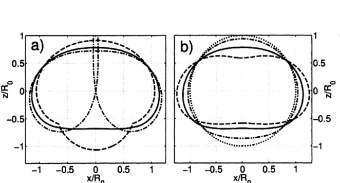
conforms to that of the substrate over the area 0 < 0 < a. . . . . 39 2-3 a) The static profiles of a liquid drop with Bo = 1 on a flat surface.
The three profiles are the sum of the first 50 spherical harmonic modes obtained by minimizing the surface and gravitational potential energy of a drop constrained in different ways, by averaging the reaction force over: the contact area (equation (2.19)) (solid line), the contact area rim (dashed line), and the center of the contact area (dash-dot line). We see that even for an 0(1) Bond number, the averaging method provides a good approximation to the actual drop shape, which has a perfectly flat base. b) The static profile of a drop obtained from the first 50 spherical harmonics using the averaging method (2.20) for several values of Bo: Bo = 0 (dotted line), Bo = 0.5 (dash-dot line),
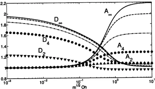
Bo = 1 (solid line) and Bo = 1.5 (dashed line). . ... 44 2-4 The dependence of the coefficients Am and Dm from equation (2.31)
on the scaled Ohnesorge number Ohm = M1/2 Oh. Curves for m =
2,4,10,40 (triangles, circles, dash-dot and dashed lines respectively) are shown, together with the limiting curves for m -+oo (solid lines) corresponding to planar surface capillary waves. ... 48 2-5 The dependence of the dissipation coefficient CD in equation (2.34) on
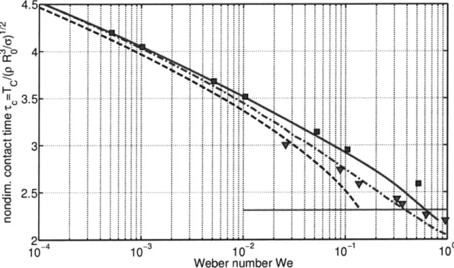
2-6 Comparison of the nondimensional contact time r, = Tc/ (pg/a)1
/2 as
a function of the Weber number We = pR Vl/2l for Oh = / (pofo)" = 0.005 and Bo = pgRg/ = 0, obtained with our quasi-static model
(2.38) (solid line), the simplified model (2.40) (dashed line) and nu-merical simulation of the first 250 spherical harmonic modes (2.42)
(dash-dot line). The predictions of Gopinath & Koch [53] (0), Foote [42] (v) and Okumura [84] (horizontal line) are included for the sake of comparison... 53 2-7 The dependence of the nondimensional contact time r, = Tc (u/pj)"2
on the rescaled Weber number We/? 2 = pR0oV2/o(1 - RO/R
2)2.
Re-sults of the numerical model (2.42) for several values (0.1 < < 5 10) of the curvature parameter 1Z = 1 - RO/R 2 follow a single curve (solid line). The analytic expression (2.43) (dashed line) is shown for the sake of comparison. . . . . 55 2-8 The effects of gravity on the nondimensional contact time rc = TC
as a function of the Weber number We = pRoVe
/a.
The results of the numerical model (2.42) (dash-dot line), quasi-static model (2.38)(solid line) and the analytical expression (2.44) (dashed line), all for Bo = 0.05 are plotted, together with the experimental results of Oku-mura et al, for Bo = 0.02 (V) and Bo = 0.05 (0). For reference, the result of the numerical model (2.42) for Bo = 0 (i.e. no gravity) is also shown (*). .. ... .. .... . .. .. .. ... .. 56 2-9 The dependence of the coefficient of restitution CR on the Weber
num-ber We = pRogV/o with (a) and without (b) gravity, for a drop
im-pacting a flat substrate (1Z = 1). Results of the quasi-static model (2.38) (solid lines) and the full numerical model (2.42) (points) are shown for four values of the Ohnesorge number Oh =
Oh = 0.1 (o), Oh = 0.2 (M), Oh = 0.3 (V) and Oh = 0.4 (A)... 57 3-1 A schematic illustration of the experimental set-up. A liquid drop
bounces on a liquid bath enclosed in a circular container shaken ver-tically. The drop is illuminated by a strong LED lamp through a diffuser, and its motion recorded by a high-speed camera that can be synchronized with the shaker. ... ... 63
3-2 A droplet of radius Ro = 0.38mm (a) in flight and (b) during contact with the bath. The drop motion is determined by the gravitational force g and the reaction force PR generated during impact. ... 63 3-3 Regime diagram describing the motion of a silicone oil droplet of
vis-cosity 50 cS on a bath of the same fluid vibrating with frequency 60Hz. The horizontal axis is the dimensionless peak acceleration of the bath P = -y/g, while the vertical axis is the drop radius. The bath surface becomes unstable when
r
exceeds the Faraday threshold Pr = 5.46 (vertical line). Only the major dynamical regimes are shown: PDC signifies the period-doubling cascade, Int the region of intermittent horizontal movement and Walk the walking regime. Lines indicate best fits to threshold curves. ... 66 3-4 The simplest modes of vertical motion for 50 cS silicone oil dropsbouncing on a liquid bath vibrating with frequency 50 Hz. These are, in order of increasing dimensionless forcing P = -y/g: (a) the (1, 1)1 mode, P = 1.3; (b) the (1, 1)2 mode, P = 1.4; (c) the (2,2)2 mode,
r
= 2.35; (d) the (2,1)1 mode, P = 3.6 and (e) the (2,1)2 mode,r
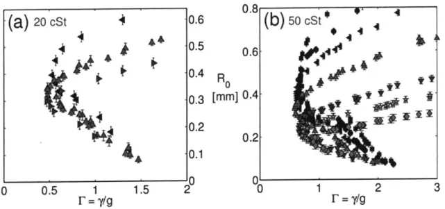
= 4.1. The drop radii are Ro = 0.28mm in (a-c) and Ro = 0.39mm in (d-e). The images were obtained by joining together vertical sec-tions from successive video frames, each one 1 pixel wide and passing through the drop's centre. The camera was recording at 4000 fps. Note that in both the (2, 1) modes shown (d-e), the drop was walking. . . 68 3-5 Bouncing thresholds measured for silicone oil droplets of viscosity (a)20 cS and (b) 50 cS on a vibrating bath of the same oil. The minimum driving acceleration
r
= iy/g (horizontal axis) required for sustained bouncing is shown as a function of the drop radius Ro (vertical axis). Experimental results are shown for several driving frequenciesf:
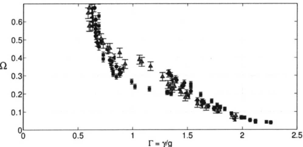
40 Hz (0), 50 Hz (*), 60 Hz (4), 80 Hz (A), 100 Hz (P), 120 Hz (V), 150 Hz (*) and 200 Hz (*). . .. . . .. 70 3-6 Bouncing thresholds. The same experimental data shown in Fig.3-5 isnow plotted as a function of the vibration number Q = w/wD (verti-cal axis) instead of drop diameter Ro. Data for different frequencies collapse nearly onto a single curve. ... 70
3-7 Detail of Fig. 3-6 showing the bouncing thresholds for silicone oil droplets of viscosity 50 cS on a vibrating bath of the same oil. The min-imum driving acceleration P = 'y/g (horizontal axis) needed to prevent the drop from coalescing with the bath is shown as a function of the vibration number Q = w/WD (vertical axis). Experimental results are shown for several driving frequencies f: 40 Hz (M), 50 Hz (*), 60 Hz (4), 80 Hz (A). The discontinuity of the bouncing thresholds between
r
= 1 andr
= 1.2 is clearly apparent . . . . 713-8 First two period-doubling thresholds for silicone oil droplets of viscos-ity (a) 20 cS and (b) 50 cS on a vibrating bath of the same oil. For smaller droplets (Q < 0.6) these are (1, 1) -+ (2, 2) and (2,2) -+ (4, 4)
transitions, while for larger drops (1 > 0.6) they are (1, 1) -+ (2,2) and (2,1) -+ (4,2) transitions. The experimentally measured thresh-old acceleration P = -y/g (horizontal axis) is shown as a function of the vibration number f = W/WD (vertical axis) for several driving
frequen-cies: f = 40 Hz (M), 50 Hz (o), 60 Hz (4), 80 Hz (A), 100 Hz (o), 120 Hz (v), 150 Hz (*) and 200 Hz (4) ... 72 3-9 A schematic illustration of our choice of coordinates. The vertical
position of the drop's centre of mass Z is equal to 0 at the initiation of impact (a), and would be -1 if it reached the equilibrium level of the bath (b). . . . . 73 3-10 Normal coefficient of restitution C = V,./V. of silicone oil droplets
impacting a bath of the same liquid, as a function of the Weber num-ber We = pRoV2/cr. Shown are results for 20 cS (M) and 50 cS
(v) droplets impacting a quiescent bath, together with values mea-sured from drops impacting a vibrating bath just above the bouncing threshold, (*) and (A), respectively. . . . . 77 3-11 Dimensionless contact time 7-c =
Tc/
(pR/a)11 2 of silicone oil dropletsimpacting a bath of the same liquid, as a function of the Weber num-ber We = pRoV2/a. Shown are results for 20 cS (U) and 50 cS (v) droplets impacting a quiescent bath, together with values mea-sured from drops impacting a vibrating bath just above the bouncing threshold, (*) and (A), respectively. . . . . 78
3-12 Comparison of the bouncing thresholds and first two period-doubling transitions measured experimentally and calculated using the linear spring model (3.1). Refer to Fig. 3-3 to see where these transitions fit into the regime diagram. The linear model predictions with CR = 0.42 and rc = 4.2 (solid lines) are compared to experiments with 20 cS oil in which coalescence (A), 1st period doubling (*) and 2nd period doubling were measured. The predictions of the model with CR = 0.32 and -rc = 4.4 (dashed lines) are compared to experiments with 50 cS oil in which coalescence (v), 1st period doubling (0) and 2nd period doubling (4)) were measured. The lines shown are, from the left, the bouncing thresholds, (1, 1)1 +- (1,1)2 mode transitions, first period-doubling (1,1) -+ (2,2) and second period-period-doubling (2,2) -+ (4,4) or (2,1) -+ (4,2). . . . . 80
3-13 Comparison of the same experimental data as in Fig.3-12 and the pre-dictions of the second linear spring model (3.6) with CR = 0.3 and rc = 4.2 (solid lines), and with CR = 0.19 and rc = 4.4 (dashed
lines). The lines shown are, from the left, the bouncing thresholds,
(1, 1)1 +- (1, 1)2 mode transitions, first period-doubling (1, 1) -+ (2,2) and second period-doubling (2,2) -+ (4,4) or (2,1) -+ (4,2). ... 81
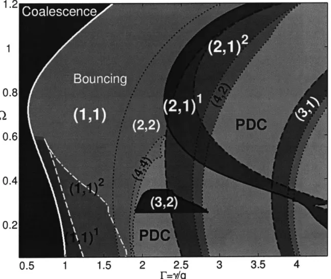
3-14 Regime diagram indicating the behaviour of a bouncing drop in the IP - Q plane, as predicted by the linear spring model (3.1) with CR = 0.42 and rc = 4.2. 0 = W/WD is the vibration number and r =
-y/g the dimensionless driving acceleration. In the (n, n) mode, the drop's motion has period equal to m driving periods, during which the drop hits the bath n times. PDC indicates a region of period-doubling cascade and chaos. Solid lines indicate lower boundaries of existence (or stability) of lower energy modes, dash-dot lines indicate upper boundaries. Similarly, dashed lines indicate lower boundaries of existence of higher energy modes, their upper boundaries being period-doubling transitions marked by dotted lines. ... 83
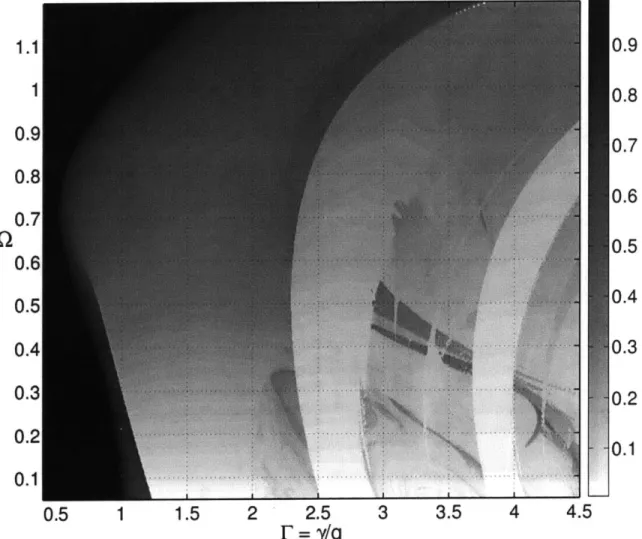
3-15 The relative contact time (fraction of the bouncing period spent in con-tact with the bath) of a bouncing drop in the r-n plane, as predicted by the linear spring model (3.1) with CR = 0.42 and rc = 4.2. 1 is the vibration number and IP the dimensionless driving acceleration. Sharp changes of the relative contact time are evident near r ; 1 (the bounc-ing to oscillatbounc-ing transition, or the (1, 1)2 - (1,1)1 mode transition),
r
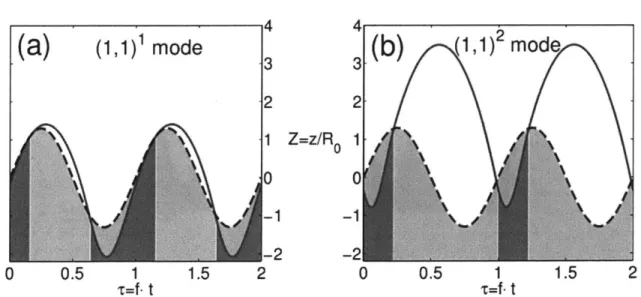
; 2.4 (onset of the (2, 1)2 mode) and F ; 3.7 (onset of the (3, 1)m ode). . . . . 84 3-16 Comparison of (a) the low energy "vibrating" (1, 1)' mode and (b)
the high energy "bouncing" (1, 1)2 mode, as predicted by the linear spring model (3.1) with irc = 4.2, CR = 0.42 for (r, 1) = (1.3, 0.35). The dimensionless vertical position of the oscillating bath (dashed line) and the droplet's center of mass shifted down by one radius (solid line) are shown as functions of the dimensionless time r = ft, where f is the bath's driving frequency. See Fig. 3-4 (a-b) for the experimental realizations of these modes. ... 85 3-17 Comparison of (a) the lower energy (2, 1)1 mode and (b) the higher
energy (2,1)2 mode, as predicted by the linear spring model (3.1) with
rc = 4.2, CR = 0.42 for (r, n) = (2.6,0.7). The dimensionless vertical position of the oscillating bath (dashed line) and the droplet's center of mass shifted down by one radius (solid line) are shown as functions of the dimensionless time r = ft. See Fig. 3-4 (d-e) for the experimental
realizations of these modes. . . . . 85 3-18 The (3,2) mode, as predicted by the linear spring model (3.1) with
rc = 4.2, CR = 0.42 for (F, 1) = (2.4,0.32). The dimensionless vertical position of the oscillating bath (dashed line) and the droplet's center of mass shifted down by one radius (solid line) are shown as functions of the dimensionless time r = ft. ... 86 3-19 The dependence of the normal coefficient of restitution CR =Vet/Ni
for silicone oil droplets impacting a bath of the same liquid, on the Weber number We = pRoV2/u. Shown are the experimental results
for 20 cS (M) and 50 cS (v) droplets impacting a quiescent bath. (*) and (A) denote analogous CR values for droplets impacting a vibrating bath just above the bouncing threshold. Solid lines indicate the values obtained using the logarithmic spring model (B.13) with RO = 0.15mm for ci = 2, c2(20 cS) = 12.5, c2(50 cS) = 7.5 and c3 = 1.4.. ... 87
3-20 The dimensionless depth of penetration
IZI
= IzI/RoWe" 2 of the drop's center of mass below its height at the outset of contact (see Fig. 3-9), as a function of the dimensionless time r = t (Cr/pR)" 2.The predictions of the linear spring model (3.1) (dashed line), alter-native linear spring model (3.6) (dash-dot line) and the logarithmic spring model (3.7) (solid line) for Ro = 0.3mm and We = 0.8 are com-pared to the experimental values for Ro = 0.14mm, We = 0.73 (N),
Ro = 0.20mm, We = 0.68 (A) and Ro = 0.33mm, We = 0.96 (1). . 88
3-21 The dimensionless acceleration Z,, = (d2z/dt2) (pRi/oVa)"2 of the drop's center of mass as a function of the dimensionless time r =
t (oa/pRi)" 2. The predictions of the linear spring model (3.1) (dashed
line), alternative linear spring model (3.6) (dash-dot line) and the
log-arithmic spring model (3.7) (solid line) are shown for RO = 0.3mm and
We = 0.8. .. ... . ... .. .... . . 89 3-22 Comparison of the regime diagrams measured experimentally and those
calculated using the logarithmic spring model (3.7). (a) The model predictions with cl = 2, c3 = 1.4, c2 = 12.5 and f = 80 Hz (solid lines) are compared to experiments with 20 cS oil in which coalescence (A), 1st period doubling (o) and 2nd period doubling (o.) were measured. (b) The predictions of the model with c, = 2, c3 = 1.4, c2 = 7.5 and
f
=
80 Hz (dashed lines) are compared to experiments with 50 cS oil in which coalescence (A), 1st period doubling (o) and 2nd period doubling (loo) were measured. . . . . 90 3-23 The dependence of the impact phase 4) (solid lines, points), definedin (3.8), on the driving acceleration
r
= -y/g for three values of the vibration number Q: (a) Q = 0.2, (b) Q = 0.5 and (c) 0 = 0.8 (refer to Fig. 3-22a). Contact is marked by the shaded regions, wherein darkness of the shading indicates the relative number of contacts including the given phase. Where possible, the periodic bouncing modes (m, n) areindicated. . . . . 92 4-1 The experimental setup. A liquid drop bounces on a vibrating liquid
bath enclosed in a circular container. The drop is illuminated by an LED lamp, its vertical motion recorded on a high-speed camera and its horizontal motion recorded on a top view camera. Both cameras are synchronized with the shaker. ... 100
4-2 A droplet of radius Ro = 0.38mm (a) in flight and (b) during contact with the bath. During flight, its motion is accelerated by the gravita-tional force g and resisted by the air drag FDA that opposes its motion
v. During contact, two additional forces act on the drop; the reaction
force F normal to the bath surface and the momentum drag force FD tangential to the surface and proportional to the tangential component of V. . . . . 100
4-3 Examples of the vertical motion of 50 cS silicone oil drops walking on a liquid bath vibrating with frequency 50 Hz. These are, in order of in-creasing complexity: (a) the (2,1)1 mode, RO = 0.39mm,
r
= 3.6; (b) the (2, 1)2 mode, R& = 0.39mm, r = 4.1; (c) the (2,2) limping mode, & = 0.57mm, r = 4.0; (d) switching between the (2, 1)' and (2,1)2 modes that arises roughly every 20 forcing periods, Ro = 0.35mm,r7=4.0; (e) chaotic bouncing, Ro = 0.57mm, r = 4.0. Here RO is the drop radius and
r,=
-y/g the dimensionless driving acceleration. The images were obtained by joining together vertical sections from suc-cessive video frames, each 1 pixel wide and passing through the drop's centre. The camera was recording at 4000 fps. ... 102 4-4 The walking thresholds for silicone oil droplets of viscosity (a) 20 cSand (b) 50 cS on a vibrating bath of the same oil. The experimentally measured threshold acceleration P = -t/g (horizontal axis) is shown as a function of the vibration number i = W/WD (vertical axis) for several values of the driving frequency f: 50 Hz (P), 60 Hz (M), 80 Hz (A) and 90 Hz (v). The dashed lines are best-fit curves provided to guide the eye. ... ... 104 4-5 The walking speed of silicone oil droplets for (a) v = 20 cS, f = 80 Hz
and (b) v = 50 cS, f = 50 Hz, bouncing on a vibrating bath of the same oil, as a function of the driving acceleration. The experimentally measured speeds are shown for several droplet radii RO. For 20 cS, Ro = 0.31 mm (v), 0.38 mm (N)
,
0.40 mm (4) and 0.43 mm (0),while for 50 cS, RO = 0.25 mm (A), 0.34 mm (Io), 0.39 mm (4) and 0.51 mm (M). In (a), the walking speeds reported by Protiere et al. [98] are shown for comparison, for drop radii 0.28 mm (A), 0.35 mm
4-6 Comparison between the full numerical model (dashed line) and the long-term approximation (C.50) (solid line) for (a) 20 cS oil and (b) 50 cS oil. The dimensionless height of the surface h(0, r) at the centre of drop impact is shown as a function of time, nondimensionalized by
the Faraday period TF = 2/f. The surface is forced at t = TF/4 and then evolves freely. ... ... 107
4-7 The tangential coefficient of restitution C = vT/o, as a function
of the normal Weber number WeN = pR0(Vj)2/o-, where vT, vN are
the tangential and normal components of the drop velocity relative to the bath surface. Data for 20 cS (v) and 50 cS (A) silicone oil are shown, together with the values obtained with the model (4.10) with C = 0.3 for Ro = 0.1 mm (solid line) and Ro = 0.4 mm (dashed line).
The impact angle with respect to the bath surface ranged from 45* to
nearly 90'. ... ... 108 4-8 The walking thresholds as predicted by (4.31) for (a) 20 cS droplets
at driving frequency f = 60 Hz (solid line), f = 80 Hz (dashed line),
f = 90Hz (dash-dot line) and (b) 50 cS droplets at f = 50 Hz (solid line) and f = 60 Hz (dashed line). These should be compared to the corresponding experimental data at driving frequency f = 50 Hz (0),
f = 60 Hz (M), f = 80 Hz (A) and f = 90 Hz (v). .
...
116 4-9 The walking speeds of silicone oil droplets for (a) Y = 20 cS, f = 80Hzand (b) v = 50 cS and f = 50 Hz, as a function of the driving acceler-ation relative to the Faraday threshold
J/rF.
In (a), the experimentaldata for Ro = 0.31 mm (V), 0.35 mm (.), 0.38 mm (P) and 0.40 mm
(4) are compared to the speeds obtained using (4.28) with sin #4 = 0.5. In (b), the experimental data for Ro = 0.25 mm (A), 0.34 mm (0), 0.39 mm (4) and 0.51 mm (U) are compared to the predictions of (4.28) with sin 4P = 0.7. ... 117 4-10 The walking thresholds for silicone oil droplets of viscosity (a) 20 cS
and (b) 50 cS on a vibrating bath of the same oil. Our model predic-tions (lines) are compared to the existing data in the
J/rF
- Q plane,where
r/rF
is the ratio of the peak driving acceleration to the Faraday threshold and Q = W/WD the vibration number. Experimental data is shown for several driving frequenciesf:
50 Hz ((O) and (>) for data from Protiere et al. [98]), 60 Hz (U), 80 Hz ((A) and (A) for data from Eddi et al. [33]) and 90 Hz (V). . . . . 1184-11 Regime diagrams delineating the dependence of the form of the drop's vertical and horizontal motion on the forcing acceleration P = -y/g and the vibration number Q. Silicone oil of viscosity 20 cS is considered and several values of the driving frequency: (a) f = 50 Hz, (b) 60 Hz, (c) 70 Hz, (d) 80 Hz, (e) 90 Hz and (f) 100 Hz. The walking regime (W) occurs primarily within the (2,1) bouncing mode regimes, and a sharp change in the slope of its boundary is evident across the border between the (2, 1)' and (2,1)2 modes. The walking regime, whose extent is seen to depend strongly on f, generally borders on chaotic bouncing regions (C) both above and below. Where available, experimental data on the first (A) and second (v) period doubling and on the walking thresholds (M) are also shown. The rightmost boundary corresponds to the Faraday threshold 1r. Characteristic error bars are shown. . . . .. . . .. . . . .. . . . 120 4-12 The walking speeds of silicone oil droplets for (a) v = 20 cS, f = 80
Hz and (b) v = 50 cS, f = 50 Hz, as a function of the dimensionless
driving acceleration. Our model predictions (lines) are compared to the existing data for selected drop radii. These are: (a) Ro = 0.31 mm (V), 0.35 mm (0), 0.38 mm (No-) and 0.40 mm (4, <); (b) Ro = 0.25 mm (A), 0.34 mm (*), 0.39 mm (4) and 0.51 mm (M). In (a), the predicted range of instantaneous walking speeds in the chaotic bouncing regime is indicated by the shaded regions. Discontinuities in slope of the theoretical curves indicate a switching of vertical bouncing modes from
(2,1)1 to (2,1)2 with increasing 1. Characteristic error bars are shown. 121
4-13 The fraction of the drop's bouncing period T spent in contact with the bath, as a function of the drop radius. Experimental results (a) for dimensionless driving r = 3.7 (V), r = 3.8 (O.), r = 3.9 (4),
r
= 4.0 (A) and r = 4.1 (M) are compared to the theoretical predictions (b) for the same set of r. The appearance of the higher energy (2, 1)2 mode (see Fig. 4-3a,b) at P = 3.9 is marked by a discrete decrease of contact time. ... .... ... .... .. .... .. . .123 4-14 The walking speeds [mm/s] obtained with our model for (a) v = 20 cS,f
= 80 Hz and (b) v = 50 cS, f = 50 Hz. The horizontal axis indicatesthe ratio of the peak driving acceleration to the Faraday threshold,
4-15 The walking region for (a-b) 20 cS and (c-d) 50 cS silicon oil drops, as predicted by our model (eqns.(4.15-4.19)). Horizontal axes indicate the driving frequency
f,
while the vertical axes indicate 0 = w/WD. In (a,c), the relative distance from walking threshold to Faraday thresh-old 1 - Pw/JFp is shown. The various modes of vertical bouncing atthe walking threshold are shown in (b,d), most significant of which are the two (2, 1) modes (resonant bouncing with the Faraday pe-riod, see Fig. 4-16a-b), and the different kinds of "limping" drops (the (2, 2),(4, 3),(4, 4) modes, Fig. 4-16d-f) where a relatively weak con-tact arises between a pair of strong concon-tacts. In general, the walking regime's lower boundary adjoins a region marked by chaotic bouncing (Fig. 4-16(c,g)). . . . . 124
4-16 The most common bouncing modes of 20 cS drops near the walking threshold. These are (a) the (2,1)' mode, (b) the (2,1)2 mode, (c) chaotic bouncing, (d) the (2,2) mode, (e) the (4,3) mode, (f) the
(4,4) mode and (g) chaotic limping. Modes (d)-(g) are referred to as "limping" modes, due to the short steps alternating with long ones. . 125
4-17 Comparison of the regime diagram for 20 cS silicone oil and f = 80 Hz, as predicted by our model, to the experimental data. The data on the bouncing threshold (o), first (A) and second (V) period doubling and on the walking threshold (U) are shown. The rightmost boundary corresponds to the Faraday threshold rF. ... 126
5-1 Walking drop of 20 cS silicone oil of radius 0.48 mm (a) before, (b) during, and (c) after an impact with a bath of the same liquid vibrating at 70 Hz.. ... ... ... ... 130
5-2 Schematic illustration of the experimental set-up. The vibrating bath is illuminated by two LED lamps, and the drop motion recorded by two digital video cameras. The top view camera captures images at 17.5 -20 frames per second, while the side view camera records at 4000 frames per second. The video processing is done on a computer. . . . 133
5-3 Regime diagrams indicating the dependence of the droplet behaviour on the dimensionless driving acceleration, P = 'y/g, and the vibration number, 1 = 2rf V/rF/. (a) The 20 cS-80 Hz combination for which
F= 4.22 i 0.05. (b) 50 cS-50 Hz for which rF = 4.23 + 0.05. (c)
20 cS-70 Hz for which Pr = 3.33 t 0.05. Filled areas correspond to theoretical predictions, the solid red line denoting the theoretically pre-dicted walking threshold. Square markers denote stationary bouncing drops; round markers indicate observed walking drops. The colour of the markers indicate the observed bouncing mode. ... 135 5-4 Some of the bouncing modes observed for the 20 cS-80 Hz combination.
(a) Bouncing (4,4) mode. F = 2.3, 1 = 0.45. (b) Bouncing (4,3) mode. P = 2.7, Q = 0.45. (c) Bouncing (4,2) mode. P = 3.5, Q = 0.42. . . . 137
5-5 Some of the modes observed for the 50 cS-50 Hz combination. (a) Walking (2,1)' mode. r = 3.7, Q = 0.59. (b) Walking (2,1)2 mode. P = 4.0, Q = 0.44. (c) Chaotic bouncing with no apparent periodicity.
r = 4, Q = 0.94.. ... 137
5-6 Some of the modes observed for the 20
cS-70
Hz combination. (a) Exotic bouncing mode (13,10): highly complex periodic motion. f =3.3, O1 = 0.97. (b) The limping drop, a (2,2) walking mode. P = 2, Q = 0.42. (c) The mixed walking state, shown here evolving from (2,1)1 -+ (2,1)2 _+ (2,1)1 -+ (2, 1)2. P = 3.4, Q = 0.72. ... 138
5-7 Mixed state walkers observed with the 20 cS-70 Hz combination, P = 3.4, Q = 0.72. (a) The trajectory for a drop in the mixed state, shaded according to the speed. The circular bath domain is indicated. (b) The observed variation of walking speed with arc-length, as normalised by the Faraday wavelength. (c) A Fourier power spectrum of the nor-malised velocity fluctuations. (d) Trajectory of a mixed mode, shaded according to speed, that destabilises into a (2, 1)2 walker after collision with the boundary near (x, y) = (-25, -20) mm. ... 139 A-1 The surface tension (a) and density (b) of silicone oil as a function
of the viscosity v. Squares indicate the values for the standard set of industrial oils with 0.65cS< v < 1000cS, while the lines indicate the fitted curves (A.1). ... ... 149
C-1 Comparison between the full numerical model and the long-term ap-proximation (C.52). The bath surface is forced at time t = timp and then evolved freely, and the amplitude of the standing wave A(t) = h(0, t) is recorded, as computed by a full numerical scheme solving (C.27) (A...) and as given by (C.52) (Ath). The average ratio Anum/Ath
over TF < t < 6TF (A) and over TF < t < 10Th (V) is shown as a function of tim,, for different combinations of oil viscosity and driving frequency: (a) v = 10 cS and f = 100 Hz, (b) v = 20 cS and f = 80
Hz, (c) v = 20 cS and f = 50 cS and (d) v = 100 cS and f = 40 Hz. The ratio tends to 1 for large times, except near timp ; TF,
when G1(timp) * 0 and other wavenumbers contribute to the overall
amplitude beside the region near kF. ... 165
E-1 The dependence of the threshold value of memory Mew at which walk-ing occurs, on the wave amplitude A and force strength k. The level sets of Mew are plotted on a log A - log k plane. ... 178 E-2 The position x(t) of the drop as a function of time for various
combi-nations of the wave amplitude A and the central force strength k: (a)
A = 0.001 and k = 0.001, (b) A = 0.1 and k = 10, (c) A = 1 and k = 0.1, (d) A = 1 and k = 1, (e) A = 1 and k = 10, (f) A = 5 and
k = 2, (g) A = 20 and k = 0.05, (h) A = 50 and k = 50. ... 181
E-3 The regime diagram deduced from solution of the system (E.6), de-scribing the behaviour of a drop walking in 1 dimension subject to central force, for Me = 109. Four different dynamical states are ob-served according to the value of the wave amplitude A (horizontal axis) and central force strength k (vertical axis): a ground state (A < 0.03 or
k > A), a chaotic ground state (k ~, A), chaotic motion k < A and
un-bounded solutions A > AC - 86.6. The regions where an asymmetric probability density was observed (for small k) are also indicated. . . . 182
E-4 The dependence of (a) (x2) and (b) P.E. - P.E. = k (T2) - kir2/4 on
the parameters A and k. By using log A + 0.05 log k for the horizontal scale, we obtain clusters of data points, each corresponding to a single value of A. ... ... 184
E-5 The position x(t) as a function of time for A = 87 and k = 100
for initial conditions x(0) = 11(0) = 12(0) = 0 and :(0) = 5. The
solution diverges from the origin starting from around t t 60, with the transition shown in more detail in the inset. ... 185 E-6 The position x(t) as a function of time for A = 80 and k = 10, for
initial conditions x(0) = 1(0) = 12(0) = 0 and i(0) = 5. The walker
slowly drifts away from the origin while oscillating rapidly, before it
snaps back to the vicinity of the origin and the process repeats. . . . 188
E-7 The limit cycle for the system (E.25) together with a part of an un-bounded trajectory starting at (y, yr, y) = (5, 0, -7) in the (y, yr, y,,)
space, shown from two different angles. . .. .. ... 189 E-8 The trajectories in the y - y, plane for the equation (E.28) with F = 1
are marked by dashed lines. The two critical points are a center at (1,0) and a saddle at (-1, 0). The periodic solution with zero time average lies very close to the homoclinic trajectory, and is indicated by a solid line. ... ... 191 E-9 The intersection of the stable manifold with the y, = 0 plane for
dif-ferent values of A: (a) A=1000, (b) A=300, (c) A=200, (d) A=120, (d) A=87, (e) A=86. The number of passages through the y, = 0, y > 0 half-plane before divergence to infinity is shown for points out-side the stable manifold. A reduction in the volume of the manifold with decreasing A is evident, together with its disappearance at A = 86.192
E-10 The y-component of the intersection of the limit cycle with the y, 0 plane as a function of A. As A is decreased progressively, the limit cycle undergoes a period-doubling cascade, and below A = 87.23 becomes a strange attractor, with windows of periodicity. The strange attractor becomes unstable at A = 86.641 ± 0.001. ... 193 E-11 The probability distribution function f(x) of the drop position x(t)
for A = 0.25, k = 0.1 and five values of the memory. These are (a) Me = 32,64,256 and (b) Me = 25, 105,106. A fast convergence to the high-memory limit is apparent. ... 194
E-12 The logarithm of the probability distribution function f(x) as a func-tion of x (vertical axis) and k (horizontal axis) for two values of A: (a) 1.58 and (b) 39.8. The horizontal scale is logarithmic, while the vertical scale indicates x13, in order to capture the profile of the distri-bution function both at small and large x. In (a) the transition from the ground state to the chaotic ground state is clearly visible near log k = 1, while the transition to a chaotic region around log k = 0.2 is more gradual. In (b) the transition to fully chaotic motion arises at log k = 1.2; at log k = -0.8 the distribution function becomes asym-m etric. . . . 195
List
of Tables
2.1 List of symbols used together with the typical values encountered in the experiments at low We reported by Okumura [84], Richard & Quere
[109] and Terwagne [116].. ... ... 38 3.1 List of symbols used together with the typical values encountered in
our experiments, as well as those reported by Eddi et al. [32] and Protiere et al. [98]. ... 65 3.2 List of variables used, along with their dimensionless counterparts.
Ro is the drop radius and WD = (a/pR8)1/2 the characteristic drop
oscillation frequency. ... ... 76 4.1 The range of driving frequencies for which drops can walk, for various
values of the oil viscosity, as reported by Protiere et al. [100]. Walking occurs for fmin f < fm,., with the minimum value of rW/rF Occur-ring at f = fwt. For f = fw,, the smallest relative driving acceleration
Fw/rF is required to produce a walking drop. The resolution of their
frequency sweep was 5 Hz. ... 103 4.2 The values of the tangential drag coefficient C used for the different
combinations of oil viscosity v and driving frequency
f
in our simulations. 117 5.1 The observed walking and bouncing modes for the three viscosity/frequencycombinations examined. Modes in bold typeface are those for which an associated spatio-temporal diagram is included (see Figs. 5-4 to 5-6).134 A.1 The physical properties of the standard set of industrial silicone oils
(polydimethylsiloxanes) at T = 25*C. The density p, surface tension a and the viscosity-temperature coefficient v(990)/v(380) are all mono-tonically increasing functions of the viscosity . . . 150
C.1 Comparison of some of the critical parameters describing the standing wave evolution, as calculated numerically and given by the theoretical approximations (C.40), (C.46), for the combinations of oil viscosity V and driving frequency f at which walking occurs. These are the Fara-day threshold rF = I'y/g, the ratio of the most unstable wavenumber
kc to the Faraday wavenumber kF, the ratio of the Faraday period
,F to the decay time r and the parameter
#1krF,
which describesthe increase of the decay rate of H(k) as k moves away from kc. The parameter E, defined in (C.41), was assumed small in our theoretical analysis. We observe a good match for small v, which gradually wors-ens as v (and thus also e) increases. The error is of order E2 . . . . . . 166 E.1 Maximum value of
Ix(t)l
for selected values of k and A below the criticalvalue AC. A rapid increase of the foray distance is evident as A -+ Ac
Chapter 1
Introduction
"Guttas in saxa cadentis umoris longo in spatio pertundere saxa."
"The drops of rain make a hole in the stone, not by violence, but by oft falling."
Lucretius, De Rerum Natura IV.
The impact of liquid drops upon liquid or solid boundaries has long been a source of fascination and inspiration. Scientific investigations of the interactions between drops, jets and liquid surfaces were initiated by Lord Rayleigh [104, 105] and Arthur M. Worthington [128, 129] in the 1870s. In order to study the dynamics of these processes, often happening over timescales too short for the human eye to perceive, they developed the technique of stroboscopy, invented by Joseph Plateau who himself was involved in the study of liquid films and droplets [92]. The stroboscope relies upon the production of a short intense burst of light, and the art of triggering and compacting the flash was perfected by Harold E. Edgerton, as evidenced by his pho-tographs of nuclear explosions. His collection of high-speed phopho-tographs [34] included captivating images of energetic drop impacts with the subsequent formation of craters with crown-like rims, and undoubtedly spurred a renewed interest in the subject.
The development and wide adoption of high-speed imaging has revealed the full range of phenomena associated with drop impact [120]. In the coalescence cascade [121, 5], a succession of progressively smaller drops is created during partial coales-cence of the original drop with a liquid bath. Following vigorous drop impact on a bath, ejecta sheets may arise [119], evolving over timescales of mere microseconds. Experimental [111, 67, 15, 58, 10, 96], theoretical [20, 84, 1, 95, 62, 14] and numerical [115, 8, 9, 70, 85] works abound, revealing and rationalizing the vast array of possi-ble behaviour and the rich physics involved. For an overview of the different impact phenomena, see Rein [106] or Yarin [131].
The impact of liquid droplets on solid and fluid surfaces is important in a
vari-ety of industrial and biological processes. Industrial applications include insecticide and pesticide design [36, 80, 127], inkjet printing [126] and fuel injection, as well as the design of airplane, ship and windmill blades [132]. For many plants and small creatures, the impact and adherence of a raindrop can lead to tissue damage or other deleterious consequences, such as compromised photosynthesis in the case of plants and respiration in the case of insects; thus, the integument of many plants and insects is hydrophobic [101, 7]. Understanding the dynamics of collisions between drops of different sizes in the atmosphere is a prerequisite to predicting the onset of rain, while raindrop impact on the sea or a puddle has major effect on the aeration of the surface layer and dispersal of spores and microorganisms. The motivation for this thesis is the hydrodynamic quantum analogue system recently discovered by Yves Couder.
In this thesis, we shall focus on drop impact on solids and fluids at relatively low impact speeds, in which both the droplet and the impactor are only weakly distorted. When the impactor is a rigid substrate, the droplet will come to rest on its surface after a series of rebounds during which its initial kinetic energy is dissipated. When the impactor is a liquid bath, the drop will eventually coalesce, after the intervening air layer separating it from the bath beneath it drains below a critical thickness [18]. However, when the bath is shaken vertically, the energy lost to dissipation and wave creation at each rebound can be offset by a transfer of kinetic energy from the bath. Thus the coalescence can be prevented, the drop being instead sustained in a bouncing motion, as was first discovered by Walker [124], since the intervening air layer does not have sufficient time to drain during impact.
As the amplitude of the bath oscillation is increased further, the drop may ex-ecute a period-doubling cascade, culminating in a chaotic vertical motion [98], a feature common to systems involving bouncing on a periodically oscillating platform [37, 73, 21]. For drops within a certain size range, the interplay between the drop and its own wave field causes the vertical bouncing to become unstable: the drop begins to move horizontally, an effect first reported by Couder et al. [19]. Note that for sufficiently high bath acceleration, known as the Faraday threshold, the bath surface becomes unstable, and a standing wave pattern emerges [38, 4]. As the bath accel-eration approaches the Faraday threshold from below, the decay rate of the surface waves created by the drop impacts is reduced and a particular wavelength is selected,
corresponding to the least stable wavenumber.
Interaction of walking drops and the surface waves reflected from the boundaries [16, 30] or from other drops [100, 98, 97, 29, 28, 32, 43, 99] leads to a variety of
interesting phenomena reminiscent of quantum mechanics [6], such as tunneling across a sub-surface barrier [30], single-particle diffraction in both single- and double-slit geometries [16] or quantization of circular orbits [43]. Considering the drop motion from a statistical perspective, interesting patterns emerge in the probability density function of the drop's position. Harris et al. showed that inside a circular corral, the density function reflects the most unstable mode of the cavity. Investigation of the drop's statistical behaviour in more complex geometries is currently underway.
The discovery of the walking drop system by Couder provided the first experi-mental realization of a pilot-wave system, first theoretically proposed by de Broglie [22] as a realist, deterministic interpretation of quantum mechanics. This pilot-wave theory for the dynamics that would underly the statistical theory provided by the standard quantum mechanics would constitute a hidden variable theory. The two crucial components of de Broglie's theory, namely the resonance between the particle and its guiding wave, and the monochromatic nature of the guiding wavefield, are both present in Couder's system. Von Neumann produced a proof [123] that osten-sibly ruled out all hidden-variable theories; however, the proof was later found to be flawed [2, 3]. Nevertheless, the prejudice against pilot-wave theory persists. It is hoped that with the insights gained from the walking drop system and the rational theory for it developed herein, this unfortunate historical legacy can be rectified.
Exploration of the possible analogies between the drop-bath system described above and quantum mechanics is a growing field of research [83, 55, 54, 56]. Com-pared to the amount of experimental work done, theoretical modeling has been lack-ing. While an early phenomenological model [100, 32] was capable of reproducing certain observed behaviours, it was unable to provide quantitative predictions of the system behaviour. The material in this thesis is intended to improve the situation by developing the first rational model of the interaction between the drop's vertical and horizontal motion, which is shown to be necessary to capture the full variety of the observed droplet behaviour. It should serve as a starting point for numerical simulations of the system [88, 75]. Moreover, it will guide the experimenters in their search for new phenomena, a goal first achieved in the results reported in chapter 4. The work presented in this thesis was motivated by the following basic questions: " Q1: When a drop is placed on a vibrating fluid bath, over what range of system
parameters will it coalesce, bounce or walk? " Q2: When it does walk, how quickly will it walk?
Chapters 3 through 5 provide the answers to these questions, while raising many new ones.
The need for predictive accuracy and numerical speed necessitated development of a new model for the drop-bath interaction, which we call the logarithmic spring
model. It is developed in three stages in chapters 2-4. In chapter 2, we treat the
normal impact of a drop on a rigid curved impactor. We there introduce our quasi-static model, which provides an adequate approximation to the drop dynamics in the limit of low impact speeds. Its application requires finding the static shape of a drop under the influence of gravity, which allows for the calculation of drop's surface and gravitational potential energy. Expressing the static shape in terms of spherical harmonics then enables us to find the kinetic energy and dissipation associated with the change of the shape within this drop shape family. Finally, the drop's equation of motion is derived and solved numerically, and its predictions are compared with the existing experimental results and numerical work. Our model captures both the effects of the substrate curvature and the drop's initial kinetic energy on the impact dynamics. Since the equations of motion show that the reaction force acting on the drop during impact is nearly linearly dependent on the deformation length, with a logarithmic correction, we dub this model the "logarithmic spring". Chapter 2 appears as published in Molakek, J. and Bush, J. W. M 2012: A Quasi-static Model of Drop Impact, Physics of Fluids 24 127103.
In chapter 3, we adapt the model in order to consider low energy drop impact on a liquid bath, as arises for walking droplets. This is achieved by extending the quasi-static approximation to the shape of the deformed bath. In order to achieve sufficient accuracy over the relatively large range of Weber numbers of interest, higher order terms are included in the equations that are fixed by matching the experimental data on the coefficient of restitution and contact time. The model is then applied to rationalize the regime diagrams describing the behaviour of drops bouncing on a vibrating bath, under the further assumption that the bath returns to its equilibrium shape between successive drop impacts. A dimensionless number defined as the ra-tio of the bath driving frequency to the drop natural oscillara-tion frequency, which we dub the vibration number, is shown to collapse the experimental data for different values of driving frequency. We predict a number of new bouncing states, as well as the coexistence of multiple bouncing states with the same periodicity but different average mechanical energy. The coalescence threshold is shown to be well captured by the model, confirming that a detailed description of the intervening air layer dy-namics is not necessary; rather, it serves only to transfer stress between droplet and
bath. Chapter 3 is currently under review at the Journal of Fluid Mechanics: Drops bouncing on a vibrating bath, Mol6bek, J. and Bush, J. W. M.
In chapter 4, we consider the spatio-temporal evolution of the bath surface after each drop impact, then the destabilizing influence of this wavefield on the bouncing states. For driving close to the Faraday threshold, the surface is found to be locally approximated by a standing wave with nearly exponential temporal decay and a radial form described by a Bessel function. By considering the horizontal force balance using a heuristic formula for the tangential drag on the drop during impact, we are able to rationalize the limited extent of the parameter range where walking occurs, as well as the speed of the walking drops. The location and extent of the walking region is found to be crucially dependent on the stability and existence of the various vertical bouncing modes. By integrating over one period of the vertical motion, the vertical dynamics can be filtered out, yielding a trajectory equation for the drop's horizontal motion. Chapter 4 is currently under review at the Journal of Fluid Mechanics: Drops walking on a vibrating bath: towards a hydrodynamic pilot-wave theory, Molshek, J. and Bush, J. W. M.
In chapter 5, we present the results of an integrated experimental and theoretical investigation of droplets bouncing on a vibrating fluid bath. A comprehensive series of experiments provides the most detailed characterisation to date of the system's dependence on fluid properties, droplet size and vibrational forcing. A number of new bouncing and walking states are reported, including complex periodic and aperiodic motions. Particular attention is given to the first characterisation of the different gaits arising within the walking regime. In addition to complex periodic walkers and limping droplets, we highlight a previously unreported mixed state, in which the droplet switches periodically between two distinct walking modes. Our experiments
are complemented by a theoretical study based on our previous developments, which provides a basis for rationalising all observed bouncing and walking states. Chapter 5 is currently under review at the Physics of Fluids: Exotic states of bouncing and walking droplets, Wind-Willassen, 0, Mohinek, J., Harris, D. M. and Bush, J. W. M. In chapter 6, we conclude our study of the bouncing and walking drops, discussing the strengths and weaknesses of our model, and proposing directions in which the theory might be extended.
Chapter 2
Drops Bouncing on a Rigid
Substrate
2.1
Background
In this chapter we treat the impact of a liquid drop on rigid or weakly-deformable substrates. The nature of small droplet collision depends on the wettability of the impacted surface, which will in general depend in turn on its surface chemistry and texture [44]. If the droplet wets the substrate, the spreading and detachment of the droplet will depend critically on the contact line dynamics [131]. In this chapter, we consider the case of non-wetting impact, in which a thin air layer is maintained between the droplet and the surface, so that contact line dynamics need not be considered. Such is the case for relatively low-energy impact of drops on super-hydrophobic surfaces [125], a rigid surface coated with a liquid film [47] or a highly
viscous liquid surface [25].
We further restrict our attention to low-energy impacts in which the droplet de-formation remains small, allowing for an analytical treatment. Two key parameters that characterize the impact are the contact time Te and the coefficient of restitution
CR. The contact time can be defined as the time over which the droplet experiences
a reaction force from the impacted object; the coefficient of restitution as the ratio of the normal components of outgoing to incoming velocity: CR = (v)na . While, strictly speaking, these definitions can only be approximate due to the interaction between drop and impactor via viscous forces in the intervening gas, for the class of problems to be considered, the resulting ambiguity is negligible.