Publisher’s version / Version de l'éditeur:
Proceedings, 2011-11-01
READ THESE TERMS AND CONDITIONS CAREFULLY BEFORE USING THIS WEBSITE. https://nrc-publications.canada.ca/eng/copyright
Vous avez des questions? Nous pouvons vous aider. Pour communiquer directement avec un auteur, consultez la
première page de la revue dans laquelle son article a été publié afin de trouver ses coordonnées. Si vous n’arrivez pas à les repérer, communiquez avec nous à [email protected].
Questions? Contact the NRC Publications Archive team at
[email protected]. If you wish to email the authors directly, please see the first page of the publication for their contact information.
NRC Publications Archive
Archives des publications du CNRC
This publication could be one of several versions: author’s original, accepted manuscript or the publisher’s version. / La version de cette publication peut être l’une des suivantes : la version prépublication de l’auteur, la version acceptée du manuscrit ou la version de l’éditeur.
Access and use of this website and the material on it are subject to the Terms and Conditions set forth at
To Aggregate or not to aggregate : that is the question
Paquet, Eric; Viktor, Herna L.; Guo, Hongyu
https://publications-cnrc.canada.ca/fra/droits
L’accès à ce site Web et l’utilisation de son contenu sont assujettis aux conditions présentées dans le site LISEZ CES CONDITIONS ATTENTIVEMENT AVANT D’UTILISER CE SITE WEB.
NRC Publications Record / Notice d'Archives des publications de CNRC:
https://nrc-publications.canada.ca/eng/view/object/?id=749f5106-d975-441a-b258-9776bfd387e8 https://publications-cnrc.canada.ca/fra/voir/objet/?id=749f5106-d975-441a-b258-9776bfd387e8TO AGGREGATE OR NOT TO AGGREGATE: THAT IS THE
QUESTION
Eric Paquet
1,2, Herna L Viktor
2and Hongyu Guo
11Institute of IT, National Research Council of Canada, Ottawa, Ontario, Canada
2Department of Electrical Engineering and Computer Science, University of Ottawa, Ottawa, Ontario, Canada
{eric.paquet, hongyu.guo}@nrc-cnrc.gc.ca, [email protected]
Keywords: Data pre-processing, aggregation, Gaussian distribution, L´evy distribution.
Abstract: Consider a scenario where one aims to learn models from data being characterized by very large fluctuations that are neither attributable to noise nor outliers. This may be the case, for instance, when examining super-market ketchup sales, predicting earthquakes and when conducting financial data analysis. In such a situation, the standard central limit theorem does not apply, since the associated Gaussian distribution exponentially suppresses large fluctuations. In this paper, we argue that, in many cases, the incorrect assumption leads to misleading and incorrect data mining results. We illustrate this argument against synthetic data, and show some results against stock market data.
1
INTRODUCTION
Aggregation and summarization is an important step when pre-processing data, prior to building a data mining model. This step is increasingly needed when aiming to make sense of massive data reposito-ries. For instance, online analytic processing (OLAP) data cubes typically represent vast amounts of data grouped by aggregation functions, such as sum and average. The same observation holds for social net-work data, where the frequency of a particular rela-tionship is often represented by an aggregation based on the number of occurrences. Furthermore, data ob-tained from data streams are frequently summarized into manageable size buckets or windows, prior to mining (Han et al., 2006).
Often, during such a data mining exercise, it is implicitly assumed that large scale fluctuations in the data must be either associated with noise or with out-liers. The most striking consequence of such an as-sumption is that, once the noisy data and the out-liers have been eliminated, the remaining data may be characterized in two ways. That is, firstly, their typical behaviour (i.e. their mean) and secondly, by the characteristic scale of their variations (i.e. their variance). Fluctuation above the characteristic scale is thus being assumed to be highly unlikely. Nev-ertheless, there are many categories of data which are characterized by large scale fluctuations. For in-stance, supermarket ketchup sales, financial data and
earthquake related data are all examples of data ex-hibiting such behaviour (Walter, 1999; Groot, 2005). The large scale fluctuations do not origin from noise or outliers, but constitute an intrinsic and distinctive feature.
Mathematically speaking, small fluctuations are modelled with the central limit theorem and the Gaus-sian distribution, while large fluctuations are mod-elled with the generalized central limit theorem and the L´evy distribution. This position paper discusses the aggregation of data presenting very large scale fluctuations, and argues that the assumption of the un-derlying Gaussian distribution leads to misleading re-sults. Rather, we propose the use of the L´evy (or sta-ble) distribution to handle such data.
2
AGGREGATION AND THE
CENTRAL LIMIT THEOREM
Aggregation is based on the standard central limit theorem which may be stated as follows: The sum of N normalized independent and identically distributed random variables of zero mean and finite varianceσ2 is a random variable with a probability distribution function converging to the Gaussian distribution with varianceσ2where the normalization is defined as in the following equation:
z=X− N hxi√ Nσ
This means that when we refer to aggregated data, in the sense of a sum of real numbers, we implic-itly assume that such aggregated data has a Gaussian distribution. This distribution is irrespectively of the original distribution of its individual data. In prac-tice, this implies that an aggregation, such as a sum, may be fully characterized by its mean and its vari-ance; this is why aggregation is so powerful. All the other moments of the Gaussian distribution are equal to zero. Despite the fact these assumptions on which aggregation is based are quite general they do not cover all possible data distributions, for instance, the L´evy distribution.
Stable or L´evy distributions are distributions for which the individual data as well as their sum are identically distributed (Samoradnitsky and Taqqu, 1994; V´ehel and Walter, 2002). That implies that the convolution of the individual data is equal to the distribution of the sum or, equivalently, that the char-acteristic function of the sum is equal to the product of their individual characteristic functions. Extreme values are much more likely for the L´evy distribu-tion that they are for the Gaussian distribudistribu-tion. The reason being that the Gaussian distribution fluctuates around its means, the scale of the fluctuations being characterized by its variance (the fluctuations are ex-ponentially suppressed) while the L´evy distribution may produce fluctuations far beyond the scale param-eter because of the tail power decay law.
The L´evy distribution is characterized by four parameters as opposed to the Gaussian distribution which is characterized by only two. The parameters are: the stability exponentα, the scale parameterγ, the asymmetry parameterβ and the localisation pa-rameter µ. While the tail of the Gaussian distribution is exponentially suppressed, the tail of the L´evy dis-tribution decays as a power law (heavy tail) which de-pends on its stability exponent, as the following equa-tion shows: Lα(x) ∼ C± |x|1+α x−→±∞
It should be noticed that the L´evy distribution re-duces to the Gaussian distribution whenα= 2 and when the asymmetry parameter is equal to zero. A L´evy distribution with 1≤α<2 has a finite mean, but an infinite variance while a distribution withα<1 has both an infinite mean and an infinite variance. As we will see in the following sections, these properties have grave consequences from the aggregation point of view.
3
SIMULATION RESULTS
In this section, we present simulations which il-lustrate our previous observations. All simulations were performed using Mathematica 8.0 on a Dell Pre-cision M6400. In the following,α= 2 corresponds to a Gaussian distribution.
3.0.1 Simulations
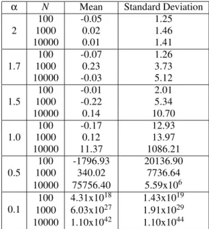
Table 1 shows the mean and the standard deviation estimated from empirical data drawn from a stable distribution for various values of the stability expo-nentαand size N. One may notice that whenα<1, the mean and the standard deviation are many orders of magnitude higher than those associated with the Gaussian distribution. This implies that the extreme values, associated with the tail of the distribution, dominate the mean and the standard deviation.
Table 1: Mean and standard deviation for the L´evy distribu-tion for various values of the stability exponent and of the size of the aggregate.
α N Mean Standard Deviation
2 100 -0.05 1.25 1000 0.02 1.46 10000 0.01 1.41 1.7 100 -0.07 1.26 1000 0.23 3.73 10000 -0.03 5.12 1.5 100 -0.01 2.01 1000 -0.22 5.34 10000 0.14 10.70 1.0 100 -0.17 12.93 1000 0.12 13.97 10000 11.37 1086.21 0.5 100 -1796.93 20136.90 1000 340.02 7736.64 10000 75756.40 5.59x10⁶ 0.1 100 4.31x10¹⁸ 1.43x10¹⁹ 1000 6.03x1027 1.91x1029 10000 1.10x1042 1.10x1044
Furthermore, the standard deviation does not con-verge whenα<2 and the mean and the standard devi-ation do not converge whenα<1 ; their estimate be-comes a meaningless random number. Consequently, if the empirical data have a L´evy distribution, the ag-gregation with the standard deviation is meaningless ifα<2 and the aggregation with the mean is mean-ingless if α<1. For instance, (Groot, 2005) has reported that supermarket sales of ketchup (tomato sauce) are characterized by a L´evy distribution with
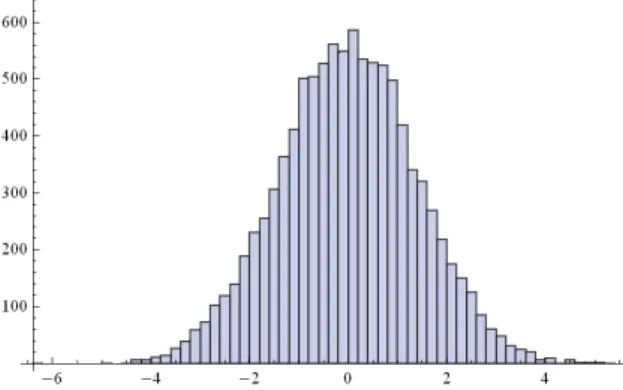
We may understand this behaviour by considering the histograms of the empirical distribution. Fig. 1 shows the histogram withα= 2 and Fig. 2 withα= 1.7. One immediately notices that the maximum of the aggregation dominates over the other values and that the scale of the fluctuations for small values of
αis many orders of magnitude higher than the one associated with a Gaussian distribution. Although the maximum of the distribution has a low probability, it totally dominates the mean and the variance ifα<1. More insight may be obtained by considering the cumulative sum of L´evy distributed data. Fig. 3 shows the cumulative sum forα= 2 and Fig. 4 for
α= 0.5. Once more, one notices the importance of the maximum which eventually tends to completely dominates the cumulative sum whenα= 0.5. Conse-quently, L´evy distributions are suitable to characterize data for which the behaviour is mostly determined, depending on the value ofα, by a limited number of extreme events.
For instance, the value of a share is usually domi-nated by a few large fluctuations and so are the dam-ages associated with earthquakes and tsunamis. When
α<1, the aggregation should be performed with the maximum function. In this particular case, the mean and the standard deviation are infinite which means that their estimations from a collection of empirical data are just meaningless random numbers. When 1≤α<2, the aggregation may be performed with the mean but the standard deviation becomes infinite.
Figure 1: Histogram of a Gaussian distribution withα= 2 and N=10000.
One should keep in mind that the closer isα to one, the slower is the convergence of the mean esti-mated on a collection of empirical data. In practice, that means that the mean should be estimated from a large number of data in order to obtain a meaningful result.
Figure 2: Histogram (notice the scale) of a L´evy distribution withα=1.7 and N=10000. 2000 4000 6000 8000 10 000 250 200 150 100 50
Figure 3: Cumulative sum for Gaussian distributed data withα=2 and N=10000. 2000 4000 6000 8000 10 000 100 100 200
Figure 4: Cumulative sum for L´evy distributed data with
α=1.7 and N=10000.
3.0.2 The L´evy Distribution and the Real World
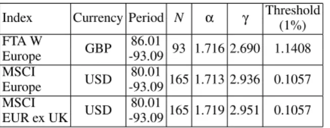
The importance of L´evy distribution is not only the-oretical. As a matter of fact, it has far reaching con-sequences for, amongst others, financial market data. With the pioneer work of Mandelbrot, it became in-creasingly apparent that financial data may be charac-terized with stable distributions. For instance, let us consider Table 2 which shows the results obtained for various Stock Market Indexes in Europe(V´ehel and Walter, 2002). Here, γ is the scale factor and the threshold is 1% (confidence level of 99%). As shown
by the data, all these indexes clearly have a L´evy dis-tribution and the value of the stability exponent is typ-ically around 1.7, which is not in the Gaussian regime.
Table 2: Estimation of the parameters of the L´evy distri-butions associated with various Stock Exchange Indexes in Europe (V´ehel and Walter, 2002).
Index Currency Period N α γ Threshold (1%) FTA W GBP 86.01 93 1.716 2.690 1.1408 Europe -93.09 MSCI USD 80.01 165 1.713 2.936 0.1057 Europe -93.09 MSCI USD 80.01 165 1.719 2.951 0.1057 EUR ex UK -93.09
Stock market data is not the only type of data that are suspect to such large data fluctuation that does not have a Gaussian distribution. As previously men-tioned, the sales of ketchup are another example of such data. Also, the damages caused by natural dis-asters such as hurricanes, tornados and earthquakes, fall within this domain. Using the standard data pre-processing techniques, and incorrectly assuming that the standard limit theorem holds in such cases, has grave impact on the validity of the resultant models constructed. This is especially true in domains where the data are aggregated prior to model building. As mentioned earlier, the vast size of massive data min-ing repositories necessitates aggregation, due to the sheer size and complexity of the data being mined.
4
CONCLUSIONS
This position paper challenges the implicit as-sumption, which is often made during numerous data mining exercises, that the standard limit theorem holds and that the data distribution is Gaussian. We discuss the implications of this assumption, especially in terms of aggregated data that is characterised with large fluctuations. We show the nature of the differ-ences between the Gaussian and L´evy distributions, on synthetic data and show an example from the real-world financial stock market data. We observe that the two sets of distributions are vastly different, and that it follows that, during any data mining exercise, that data with a Levy distribution should be treated with caution, especially during data pre-processing and ag-gregation.
The implications and applications of this observa-tion are far-reaching in many domains. It has been shown that the value of a share is usually dominated by a few large fluctuations. Damages associated with earthquakes and tsunamis, such as those caused by
the recent events in Japan, are also characterized by such large fluctuations. The same observation holds, e.g., when observing the sizes of solar flares or craters on the moon, as well as for the data obtained from many climate change studies. This fact needs to be taken into account, when aiming to create valid data mining models for these types of domains, which are becoming increasingly important for socio-economic reasons.
REFERENCES
Groot, R. D. (2005). L´evy distribution and long correlation times in supermarket sales. Lvy distribution and long
correlation times in supermarket sales, 353:501–514.
Han, J., Kamber, M., and Pei, J. (2006). Data Mining:
Con-cepts and Techniques (2nd edition). Morgan
Kauff-man.
Samoradnitsky, G. and Taqqu, M. (1994). Stable Non-Gaussian Random Processes: Stochastic Models with Infinite Variance. Chapman & Hall, New York.
V´ehel, J. L. and Walter, C. (2002). Les march´es fractals
(The fractal markets). Universitaires de France, Paris.
Walter, C. (1999). L´evy-stability-under-addition and fractal structure of markets: implications for the investment management industry and emphasized examination of matif notional contract. Mathematical and Computer