Publisher’s version / Version de l'éditeur:
Vous avez des questions? Nous pouvons vous aider. Pour communiquer directement avec un auteur, consultez la première page de la revue dans laquelle son article a été publié afin de trouver ses coordonnées. Si vous n’arrivez pas à les repérer, communiquez avec nous à [email protected].
Questions? Contact the NRC Publications Archive team at
[email protected]. If you wish to email the authors directly, please see the first page of the publication for their contact information.
https://publications-cnrc.canada.ca/fra/droits
L’accès à ce site Web et l’utilisation de son contenu sont assujettis aux conditions présentées dans le site LISEZ CES CONDITIONS ATTENTIVEMENT AVANT D’UTILISER CE SITE WEB.
Construction Research Congress 2010: 8 May 2010, Banff, Alberta [Proceedings], pp. 1-10, 2010-05-08
READ THESE TERMS AND CONDITIONS CAREFULLY BEFORE USING THIS WEBSITE.
https://nrc-publications.canada.ca/eng/copyright
NRC Publications Archive Record / Notice des Archives des publications du CNRC :
https://nrc-publications.canada.ca/eng/view/object/?id=abac0487-7f4c-434b-aea6-9575a5866eba https://publications-cnrc.canada.ca/fra/voir/objet/?id=abac0487-7f4c-434b-aea6-9575a5866eba
NRC Publications Archive
Archives des publications du CNRC
This publication could be one of several versions: author’s original, accepted manuscript or the publisher’s version. / La version de cette publication peut être l’une des suivantes : la version prépublication de l’auteur, la version acceptée du manuscrit ou la version de l’éditeur.
Access and use of this website and the material on it are subject to the Terms and Conditions set forth at
A new approach for resource-constrained multi-project scheduling
http://www.nrc-cnrc.gc.ca/irc
A ne w a pproa c h for re sourc e -c onst ra ine d m ult i-proje c t sc he duling
N R C C - 5 3 2 2 4
Z h u , J . ; L i , X . ; H a o , Q . ; S h e n , W .
M a y 2 0 1 0
A version of this document is published in / Une version de ce document se trouve dans:
Banff, Alberta, May 8-11, 2010, pp. 1-10
The material in this document is covered by the provisions of the Copyright Act, by Canadian laws, policies, regulations and international agreements. Such provisions serve to identify the information source and, in specific instances, to prohibit reproduction of materials without written permission. For more information visit http://laws.justice.gc.ca/en/showtdm/cs/C-42
Les renseignements dans ce document sont protégés par la Loi sur le droit d'auteur, par les lois, les politiques et les règlements du Canada et des accords internationaux. Ces dispositions permettent d'identifier la source de l'information et, dans certains cas, d'interdire la copie de documents sans permission écrite. Pour obtenir de plus amples renseignements : http://lois.justice.gc.ca/fr/showtdm/cs/C-42
A New Approach for Resource-Constrained Multi-project Scheduling
Jie Zhu1, Xiaoping Li1,2, Qi Hao2, Weiming Shen2
1
School of Computer Science and Engineering Southeast University, Nanjing, China
2
Centre for Computer-assisted Construction Technologies National Research Council, London, Ontario, Canada
Abstract
Construction and facilities maintenance projects involve a large number of people and tasks with resource constraints and precedence constraints. This paper presents a new approach to model this problem as a resource-constrained multi-project scheduling problem (RCMPSP) with cost minimization. The scheduling problem is first decomposed into two sub-problems: schedule generation and sequencing. For the schedule generation problem, an effective forward and reverse schedule generation (FRSG) method is developed to generate a feasible solution for a given valid sequence. For the sequencing problem, a novel complete local search with memory approach embedded with FRSG is proposed to find the solution which has the best objective value. The proposed approach has been tested on the benchmark instances. Computational results show that it performs very well in terms of both effectiveness and efficiency.
Keywords: Multi-project management, resource-constrained scheduling, cost
minimization, facilities maintenance 1. Introduction
Construction and facilities maintenance projects usually involve a large number of people and tasks with resource constraints and precedence constraints. This problem can be modeled as a resource-constrained multi-project scheduling problem (RCMPSP). The objective of multi-project scheduling is to allocate available resources to multiple projects and tasks with the highest efficiency and cost effectiveness. The problem belongs to the class of NP-hard [1] problems and it is very difficult to solve. Considerable efforts have been devoted to deal with the classical resource-constrained project scheduling problem (RCPSP) throughout the past decades [2-3]. Similar to machine scheduling, a representation was introduced for project scheduling. Classical project scheduling models were classified, along with their algorithms being surveyed. New models were also investigated for various applications. Other than these efforts, the research interest has been broadened to incorporate additional constraints from industrial applications, including: a pair of
activities must be separated by at least a given duration [4]; activities can be split during scheduling under situations where resources may be temporarily unavailable [5]; a schedule-dependent setup time is required depending on the assignment of resources to activities overtime [6].
Because of the complexity of RCMPSP problems, heuristic-based methods become very promising to construct a feasible and robust algorithm. Most of the existing heuristics methods can be roughly classified into two categories: the priority rule-based methods and the meta-heuristic-based approaches (such as genetic algorithms). Mendes [7] proposed a genetic algorithm in which the chromosome representation is based on random keys and the priorities of the activities are defined by a genetic algorithm. Mika [8] adopted simulated annealing and tabu search for a multi-mode RCPSP with discounted cash flows.
In this paper, a complete local search with memory approach is proposed for the resource-constrained multi-project scheduling problem (RCMPSP). The objective function is to minimize the cost of facilities maintenance considering setup cost, idle cost, and resource rate.
The rest of the paper is structured as follows: Section 2 presents a problem statement; Section 3 proposes a forward and reversed schedule generation (FRSG) method; Section 4 and Section 5 describe the proposed schedule generation approach and a complete local search with memory algorithm; Section 6 shows some experimental results; and finally, Section 6 provides some concluding remarks.
2. Problem Statement
The foundation of our work is based on the concept of task network. A traditional task network is composed by a set of tasks and a set of precedence relationships between the tasks. Precedence constrains the schedule in that an activity cannot start until all of its predecessors have finished. However, activities do not get completed on their own; instead, they consume resources during their progress. The scheduling problem becomes difficult to solve when the required resources have limited capacities because allocating scarce resources among competing activities adds significant complexity to the optimization objectives. We can transfer the RCMPSP to a classical RCPSP problem by combining all projects as one super project which contains all tasks from different projects as its activities. The resultant RCPSP problem for the above super project is NP-hard in strong sense and it is described as follows.
Let denotes the set of activities to be scheduled and
be the set of resources. Activities and
} 1 , , , 1 , 0 { + = n n J L } k , , 1 {
K= L 0 n+1 have a zero duration and
represent two dummy activities – dummy source and dummy sink, respectively. The activities are interrelated by two types of constraints:
(1) Precedence constraints force each activity to be scheduled after all
predecessor activities are completed;
j
j
P
(2) Activities require resources with limited capacities.
While being processed, activity requires units of resource during
the whole period of its duration . The assumption we made is that no preemption
is allowed. Resource type has a limited capacity of available all the time. The
j rj,k k∈K
j
d
k Rk
parameters , and are supposed to be integer, non-negative and
deterministic. For the dummy source and the dummy sink, we have and
for all . The precedence constraint denoted by
records all precedence relationships among activities.
j d 0 , J ∈ k j r, } j P ( [1 k R K ∈ ) ] 0 1 0=dn+ = d , 1 , 0k =rn+ k = r | ) , {(i j j A= k [n i∈
Solving the RCPSP problem means finding a schedule for the activities, taking into account precedence and resource constraints, while minimizing a certain objective function. Figure 1 shows an example of a project network, where the activities are presented on nodes and precedence are on directed arcs. A project
network is denoted as . The resource requirements are given to top of each node
and the total available numbers of resources are provided at the bottom of the network.
PN
Figure 1 A project network example
In the FM system, solutions are represented in form of a precedence-feasible
activity sequenceπ π ],L,π where π[i]∈J and i is the index of an activity in the
sequence. The precedence-feasible activity sequence is a sequence of activities satisfying the precedence constraints, i.e. any activity must have all its predecessors sequenced ahead. In the context of this paper, a precedence-feasible activity sequence
is also called a valid sequence for short. For example, and
are two valid sequences for the example project network in Figure 1. ) 10 , 9 , 8 , 7 , 6 , 5 , 3 , 2 , 4 , 1 ( ) 10 , 9 , 3 , 8 , 7 , 4 , 1 , 6 , 5 , 2 ( ] [i t
Let represent the start time of activity π[i]. A schedule for a valid sequence
can be represented by a vector of start times (t ). For the same example, Figure
2 shows a feasible schedule with the makespan of 17.
] ] 1 [ ,L,t[n
The RCPSP can be decomposed two sub-problems: (1) the schedule generation problem, in which a feasible schedule for a given valid sequence is calculated and (2) the sequencing problem, in which a valid sequence is found to have the optimal schedule. The schedule generation problem is embedded in the sequencing problem. A forward and reverse schedule generation method is developed for the schedule generation problem and a complete local search with memory is proposed for the sequencing problem.
Figure 2 The Gantt chart of a feasible schedule with the makespan of 17 3. A Forward and Reverse Schedule Generation Method
Given a valid sequence, a schedule generation method is to generate a feasible schedule for the sequence and evaluate the obtained schedule. Two kinds of schedule generation schemes are adopted in the system: forward schedule and reverse schedule.
3.1 Forward Schedule Generation Procedure
A forward schedule is a mapping where are mapped to a set of
start times which are set to be as early as possible while obeying the resource constraints. The forward schedule generation procedure is described in Figure 3.
F
S π[1],L,π[n]
ProcedureFSG(π,A)
/*π is a valid sequence and A is the set of all precedence
constraints in the project*/ 1. t[0]←0;
2. For i=1 to n+1
Find the earliest feasible start time t[i] for π[i]; 3. Return t[0],L,t[n+1]
Figure 3 Procedure for calculating the forward schedule 3.2 Reverse Schedule Generation Procedure
The reverse schedule is developed based on the forward schedule scheme by
reversing all the precedence in the project network and the given valid sequence. A
reversed project network is the network with all the precedence linkages
reversed, i.e. an activity’s predecessors in the original network become successors and its successors are changed to predecessors (as shown Figure 4). The reversed
precedence constraint set can be obtained by . Similarly, a
reverse sequence is to reverse the order of activities in the valid sequence, i.e.
. For example, the reverse of the sequence is .
R S PN R A R } ) , ( | ) , {(j i i j A AR ← ∈ ) 4 , 3 , 2 , 1 ( (4,3, R π ] 1 [ ] [ n i R i ←π +− π 2,1)
Theorem If is a precedence-feasible sequence for the project network ,
then must be a precedence-feasible sequence for .
π PN
R
π R
PN
Proof Suppose the index of an activity in and i π πR is denoted as index(i) 4
and indexR(i), respectively. For any (i,j)∈A, index(i)<index(j) must be satisfied
since π is a precedence-feasible sequence. Because is obtained by reversing
all precedence constraints, i.e. , for any ,
must be true. Since , then
must be true. Therefore, must be a precedence-feasible
sequence for . □ R PN } ) , ( | i j ∈A ) 1 ( ) (i n indexR = + R π ) , {( ij AR ← R A i j, )∈ ( ) ) j index ( index R PN ( ) (i <index ) (j index R < (i index − ) i R
The procedure to generate a reverse schedule is described in Figure 5.
Figure 4 The reverse project network and reverse sequence
ProcedureRFSG(π,A)
/*π is a valid sequence and A is the set of all precedence
constraints in the project*/
1. AR ←{(j,i)|(i,j)∈A}, [] [n 1−i]( 0, , 1 R i ←π + π i= Ln+ ) ] 1 [ ' ] 1 [ + − + −tn dn ); 2. , ,[' ]) ( , ; ' ] 1 [ R n FSG t ← π L AR) , , max ] 0 [ ]−d LC (t C 0 [ t 3. ' ; ] 1 [ max←tn+ 4. ],L,t[n+1] ( ' 0 [ max− ← C t 5. Return t[0],L,t[n+1]
Figure 5 Procedure for calculating the reverse schedule
Step 4 in Figure 5 guarantees the timetable returned by RFSG(π, A) is the
feasible timetable of π for the project network PN .
3.3 The Definition of the Objective Function
The classical RCPSP considers makespan as its objective function, i.e., the completion time of the last activity. But in the real world, cost has a higher priority to consider. In the facilities maintenance management system, three economic factors are concerned, i.e., setup cost, idle cost, and resource rate.
Setup cost is the cost for preparing and initiating a resource. denotes the
setup cost of a resource . If two consecutive activities are processed on the
setup k
C K
same resource with the waiting time less than a certain threshold, only one setup cost
is charged. The waiting time threshold is denoted as .
setup k C { 1= < I setup λ i l l ≠ j p×l e
Idle cost is charged when a resource is not used by any of the activities.
denotes the idle cost of a resource .
idle k
C K
k∈
For certain types of resources such as crafts and labor, the resource rate is calculated based on payment rates that are checked out every time increment. Such kind of resources has no idle cost, but the length of their continuously working time affects greatly on the project budget. Resource rate is the cost for continuously using a resource per time increment. The total resource utilization cost is calculated based on time increments and a portion of the time increment will be rounded into a full
time increment. denotes the payment rate and denotes the time increment
for a resource . For a resource which keeps working for time units, the
total rate cost is .
rate k C K ∈ rate k C × rate k λ k k m
⎡
rate⎤
k m/λIn order to take these three cost aspects into account for the optimization, the resource assignment interval list should be discussed first.
Figure 6 An example of the resource utilization distribution list
The resource utilization distribution list is a set of binary vectors
which means the number of resources being used during interval is .
describes the profile of the Gantt chart on resources . For the sake of convenience,
two consecutive vectors do not share the same value of , i.e., any two consecutive
vectors and must have . For example,
(as shown in Figure 6) for the schedule in Figure 2.
k I , 12 [ > <[s ],,e l l Ik k > 3 ], ] , [ es k } > l > <[si,ei],li 3 ], 6 , 5 [ , 1 ], > < <[sj,ej],lj 12 , 11 [ , 2 ], >< j , 5 , 0 [ > <[6,11 >,< 15],1
Based on , the total setup cost on resource can be calculated by the
function in Figure 7.
k
I k
Function TotalSetupCost(k) 1. TSC←0; 2. For i=0 to |Ik|−1 2.1 i, setup k l C TSC TSC← + × X ←0 2.2 For j= i−1 to 0 If si−ej <=λsetupk , ; k setu e overch C X arg ←
If Xovercharge>X, X ←Xovercharg
Else break; 2.3 TSC←TSC−X
3. Return TSC
Figure 7 Procedure for calculating the reverse schedule
k can be calculated by
∑
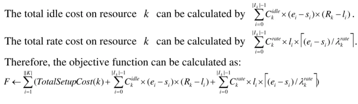
. − = − × − × 1 | | 0 ) ( ) ( k I i i k i i idle k e s R l CThe total idle cost on resource
k can be calculated by .
The total rate cost on resource
∑
⎡
⎤
− = − × × 1 | | 0 / ) ( k I i rate k i i i rate k l e s C λ
⎡
⎤
∑
∑
∑
= − = − = − × × + − × − × + ←|| | 1 1 | | 0 1 | | 0 ) / ) ( ) ( ) ( ) ( ( K i I i rate k i i i rate k I i i k i i idle k k k s e l C l R s e C k Cost TotalSetup F λ F S R STherefore, the objective function can be calculated as:
3.4 Forward and Reverse Schedule Generation Method
The procedure of the forward and reverse schedule generation method consists of three steps:
1) Calculate the forward schedule of the given valid sequence and its
objective function value.
2) Calculate the reverse schedule of the given valid sequence and its
objective function value.
3) The schedule with the smaller objective function value is selected as the final schedule of the given sequence.
4. The Complete Local Search with Memory Method
There are three containers in the algorithm: (1) NEWGEN, which accommodates the newly found valid sequences which will be explored in the current iteration; (2) NEIGHBOR, which accommodates the neighbors of the sequences in NEWGEN; and (3) DEAD, which accommodates all the explored valid sequences to avoid recalculating.
CLLM starts with a random valid sequence as the initial solution and puts it into NEWGEN. DEAD and NEIGHBOR are all empty at the beginning. The following process is iterated:
1) Generate valid sequence for NEWGEN.
a. If NEWGEN is empty, the algorithm stops;
b. The algorithm generates neighbors for all solutions in NEWGEN and check
for their validness so that only the precedence-feasible neighbors are put into NEIGHBOR; if NEIGHBOR is not full. Two methods are used to generate potential neighbors: one-insertion and the partial pair-wise exchange. The former method simply picks up an activity and moves it to every possible slot once at a time; the latter one generates neighbors by just swapping two activities in the sequence.
2) Empty NEWGEN.
3) Look through sequences contained in NEIGHBOR and check whether they are “good” enough.
a. Check each valid sequence in NEIGHBOR; if it is not in DEAD, we assume
it is “good”.
b. Calculate a schedule for a “good” sequence using the forward and reverse
c. The schedules with objective function value lower than a certain threshold value are transported to NEWGEN for the next iteration and the others are moved into DEAD. We notice that a small threshold value (for example, the best-so-far objective function value) turns the algorithm to a greedy search and stops very soon whereas a large-enough threshold value could lead to an
enumerative search. Therefore, we use F×(τ +1) as the threshold value where
is the best-so-far objective function value and the speed of search and optimality of the solution can be adjusted by factor
F
τ. 4) Empty NEIGHBOR.
If no improvement has been made for a certain number of successive iterations
max
N , the algorithm stops; otherwise go to the first step and repeat the process.
5. Computational Experiments
The proposed algorithm was implemented in Java on a Pentium 4 processor with the operating system, Windows XP. The algorithms are tested on the well-known benchmark instances [9]. Three levels of the number of activities are selected at 30, 60, 90 for the J30, J60, J90 problem sets, respectively. Each of the set contains 480 instances.
The experimental results are evaluated by a percentage relative deviation to the initial solution (PRDI), defined as follows.
% 100 × − = I I ALG F F F PRDI ALG
F is the objective function value of a solution obtained by the proposed
algorithm. I
F is the objective function value of the initial solution.
To determine reasonable parameters for the proposed CLM, 10 small instances
(j301.1-j301.10) are tested with a variety of parameters. Those parameters are τ( the
threshold value factor) and Nmax (the maximum number of non-improved iterations).
All experiments are repeated 10 times. Parameters are selected according to their effects on APRDI (average percentage relative deviation to initial solution) and CPU is the time requirement of the solutions, where APRDI is defined as follows.
% 100 × − = I IAVG F F F APRDI Where AVG
F is the average objective function value for an instance, which
implies the overall performance of the algorithm.
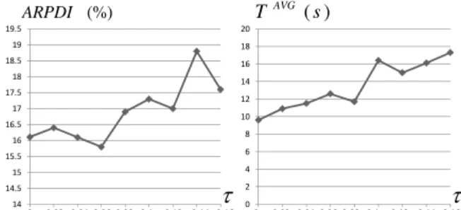
The threshold value Fbest×(τ+1) decides if a solution is good or not (Fbest is
best-so-far objective value). The algorithm becomes a greedy search when the threshold value is small (for example, the best-so-far objective value) and stops very soon, whereas the algorithm becomes an enumerative search if the threshold is large
enough. Figure 8 indicates that the bigger τ the better results, the bigger τ the
more time-consuming. To balance the efficiency and the effectiveness of the algorihm,
according to the experiments, 0.1 is reasonable for τ.
max
N is one of the termination conditions. It exerts influence on both the
efficiency and effectiveness of the algorithm. Figure 9 indicates that the larger Nmax,
0 0.02 0.04 0.06 0.08 0.1 0.12 0.14 0.16 14 14.5 15 15.5 16 16.5 17 17.5 18 18.5 19 19.5 0 0.02 0.04 0.06 0.08 0.1 0.12 0.14 0.16 τ (%) ARPDI 0 2 4 6 8 10 12 14 16 18 20 τ ) ( s TAVG
Figure 8 APRDI and the CPU time with different
τ
the better the results, the more CPU time. Therefore, Nmax is set to 50 which sets a
good trade-off between the efficiency and the effectiveness.
0 10 20 30 40 50 60 70 80 90 100 max N max N (%) ARPDI T AVG ( s) 0 5 10 15 20 25 0 2 4 6 8 10 12 14 16 18 0 10 20 30 40 50 60 70 80 90 100
Figure 9 APRDI and the CPU time with different Nmax
Based on the above the parameters, all the total 1440 instances are tested with the
results shown in Table 1. 4 measurements are taken into account, which are ARPDI,
best
PRDI ( the largest PRDI value), AVG
T ( the average CPU time, in seconds) and best
T
( the best CPU time, in seconds).
Table 1 Experimental results
n ARPDI(%) best(%) PRDI TAVG(s) ) (s Tbest 30 15.2 40.6 27 0.7 60 14.1 37.8 128.7 9.4 90 13.2 34.6 266 41.9
Table 1 illustrates that the proposal algorithm can achieve the improvement of 15.2% in average for small instances of size 30, where the best improvement percentage is 40.6%. The CPU time requirement is 27 seconds in average and merely 0.7 second for some instances. For instances of size 60, the proposed algorithm can improve the initial solution by 14.1% in average and 37.8% at most. The CPU time requirement for J60 is 128.7 seconds in average and 9.4 at least. For the large instances of size 90, the proposed algorithm can achieve the improvement of 13.2% in average and 34.6% at most. The CPU time requirement for J90 is 266 seconds in average and 41.9 seconds at least.
6. Conclusions
In this paper, a complete local search with memory algorithm is proposed for the resource-constrained multi-project scheduling problem. The goal is to minimize the objective function value which involves applicable economic factors such as setup cost, idle cost, and resource rate. A generic meta-heuristic framework for the
10
considered problem is adopted by decomposing the problem into the schedule generation problem and the sequencing problem, which are then solved by an effective forward and reverse schedule generation (FRSG) method and the proposed complete local search with memory (CLM), respectively. The proposed algorithm has been tested on the well-known benchmark instances. Reasonable parameters of CLM are determined by experiments to get a good balance between effectiveness and efficiency. For each instance, the final objective function value found during the search process is compared to the one of the initial solution to show the improvement that the algorithm can achieve. Meanwhile, since the CPU time consumed by the complete search increases significantly with the problem size, computation time is chosen as another indicator for measuring the algorithm’s performance. The experiment results also prove the applicability for using the proposed approach in facilities maintenance management.
References
[1] J. Blazewicz, J.K. Lenstra, A.H.G. Rinnooy Kan. Scheduling subject to resource constraints: Classification and complexity. Discrete Appl. Maths 1983; 5:11-24. [2] W. Herroelen, B. De Reyck, E. Demeulmeester. Resource-constrained project
scheduling: A survey of recent development. Computers&Operations Research. 1998; 25(4):279-302.
[3] J. Weglarz. Project Scheduling: Recent models, algorithms and applications. Norwell, MA: Kluwer, 1999.
[4] K. Moumene, J.A. Ferland. Activity list representation for a generalization of the resource-constrained project scheduling problem. European Journal of Operational Research 2009; 199(1):46-54.
[5] J. Buddhakulsomsiri, D.S. Kim. Properties of multi-mode resource-constrained project scheduling problems with resource vacations and activity splitting. European Journal of Operational Research 2006; 175:279-95.
[6] M. Mika, G. Waligora, J. Weglarz. Tabu search for multi-mode resource- constrained project scheduling with schedule-dependent setup times. European Journal of Operational Research 2008; 187:1238-50.
[7] J.J.M. Mendes, J.F. Goncalves, M.G.C. Resende. A random key based gentic algorithm for the resource constrained project scheduling problem. Computer&Operations Research 2009; 36:92-109.
[8] M. Mika, G. Waligora, J. Weglarz. Simulated annealing and tabu search for multi-mode resource-constrained project scheduling with positive discounted cash flows and different payment models. European Journal of Operational Research 2005; 164:639-68.
[9] R. Kolisch, A. Sprecher, A. Drexl. Characterization and generation of a general class of resource-constrained project scheduling problems. Management Science 1995; 41:1693-703.