BEAM-FORMING ERRORS IN MURCHISON WIDEFIELD
ARRAY PHASED ARRAY ANTENNAS AND THEIR
EFFECTS ON EPOCH OF REIONIZATION SCIENCE
The MIT Faculty has made this article openly available.
Please share
how this access benefits you. Your story matters.
Citation
Neben, Abraham R., Jacqueline N. Hewitt, Richard F. Bradley,
Joshua S. Dillon, G. Bernardi, J. D. Bowman, F. Briggs, et al.
“BEAM-FORMING ERRORS IN MURCHISON WIDEFIELD ARRAY
PHASED ARRAY ANTENNAS AND THEIR EFFECTS ON EPOCH OF
REIONIZATION SCIENCE.” The Astrophysical Journal 820, no. 1
(March 17, 2016): 44. © 2016 The American Astronomical Society
As Published
http://dx.doi.org/10.3847/0004-637x/820/1/44
Publisher
iop
Version
Final published version
Citable link
http://hdl.handle.net/1721.1/102669
Terms of Use
Article is made available in accordance with the publisher's
policy and may be subject to US copyright law. Please refer to the
publisher's site for terms of use.
Research School of Astronomy and Astrophysics, Australian National University, Canberra, ACT 2611, Australia
9
MIT Haystack Observatory, Westford, MA 01886, USA
10Raman Research Institute, Bangalore 560080, India 11
Harvard-Smithsonian Center for Astrophysics, Cambridge, MA 02138, USA
12
Department of Physics, University of Washington, Seattle, WA 98195, USA
13
School of Chemical & Physical Sciences, Victoria University of Wellington, Wellington 6140, New Zealand
14
Department of Physics, University of Wisconsin–Milwaukee, Milwaukee, WI 53201, USA
15
CSIRO Astronomy and Space Science(CASS), P.O. Box 76, Epping, NSW 1710, Australia
16
National Centre for Radio Astrophysics, Tata Institute for Fundamental Research, Pune 411007, India
17
International Centre for Radio Astronomy Research, Curtin University, Bentley, WA 6102, Australia
18
School of Physics, The University of Melbourne, Parkville, VIC 3010, Australia Received 2015 October 22; accepted 2016 February 5; published 2016 March 16
ABSTRACT
Accurate antenna beam models are critical for radio observations aiming to isolate the redshifted 21 cm spectral line emission from the Dark Ages and the Epoch of Reionization (EOR) and unlock the scientific potential of 21 cm cosmology. Past work has focused on characterizing mean antenna beam models using either satellite signals or astronomical sources as calibrators, but antenna-to-antenna variation due to imperfect instrumentation has remained unexplored. We characterize this variation for the Murchison Widefield Array (MWA) through laboratory measurements and simulations,finding typical deviations of the order of ±10%–20% near the edges of the main lobe and in the sidelobes. We consider the ramifications of these results for image- and power spectrum-based science. In particular, we simulate visibilities measured by a 100 m baseline andfind that using an otherwise perfect foreground model, unmodeled beam-forming errors severely limit foreground subtraction accuracy within the region of Fourier space contaminated by foreground emission(the “wedge”). This region likely contains much of the cosmological signal, and accessing it will require measurement of per-antenna beam patterns. However, unmodeled beam-forming errors do not contaminate the Fourier space region expected to be free of foreground contamination(the “EOR window”), showing that foreground avoidance remains a viable strategy.
Key words: cosmology: observations – dark ages, reionization, first stars – instrumentation: interferometers – methods: statistical– techniques: interferometric
1. INTRODUCTION
Efforts to observe the formation of the first galaxies during the Dark Ages and the subsequent Epoch of Reionization (EOR) are at the frontier of observational cosmology. Tomographic maps of neutral hydrogen in the intergalactic medium at these redshifts, where the majority of the observable comoving volume of the universe resides, will shed light on questions ranging from astrophysics and cosmology to particle physics (see Furlanetto et al. 2006; Morales & Wyithe2010; Pritchard & Loeb2012; Loeb & Furlanetto2013; Zaroubi2013 for reviews). The extreme brightness temperature sensitivity needed to isolate this faint signal in the presence of bright galactic and extragalactic radio emission (foregrounds) and detector noise necessitates thousand-hour integrations and
hundreds of antenna elements (e.g., Parsons et al. 2012a; Beardsley et al. 2013; Thyagarajan et al. 2013; Pober et al. 2014). This quest is highlighting the characterization of antenna beam patterns, or primary beams, as crucial for high dynamic range calibration and foreground subtraction(Jacobs et al.2013; Moore et al. 2013; Thyagarajan et al.2015b, and Pober et al.2016).
Two types of antenna mismodeling are relevant: (1) mismodeling of the mean antenna beam pattern; and (2) neglect of antenna-to-antenna variation. Both limit calibration and foreground subtraction fidelity in ways ranging from the obvious effect of subtracting sidelobe sources with the wrong apparentfluxes to the uncertain manner in which beam-related calibration errors average down with time. Indeed, modeling of antenna-to-antenna variation was long suspected to be critical for 21 cm observatories, and early analysis pipeline develop-ment focused on incorporating knowledge of per-antenna
19
beams in data reduction (Morales & Matejek 2009; Sullivan et al. 2012), or even fitting for them in real time (Mitchell et al.2008).
The Murchison Widefield Array (MWA) (Lonsdale et al. 2009; Bowman et al.2013; Tingay et al.2013) is now operating along with other instruments such as the Precision Array for Probing the Epoch of Reionization (PAPER) (Parsons et al. 2010, 2014) and the LOw Frequency Array (LOFAR; van Haarlem et al.2013). Analysis of the data from these arrays is bringing new urgency to the question of antenna beam patterns. Source-based methods have long been used to constrain the mean antenna beam using interferometer cross-correlations (visibilities; e.g., Pober et al.2012; van Haarlem et al. 2013; Colegate et al. 2014). More recently, working toward in situ measurements of per-antenna beams both for the MWA and for the developing next generation Hydrogen Epoch of Reionization Array(HERA; Backer et al.2009; Pober et al. 2014; De Boer et al. 2016, in preparation), Neben et al. (2015, 2016) present a beam measurement system using the ORBCOMM satellite constellation, an idea also explored by (Zheng et al.2014). Development of a drone equipped with a radio transmitter is also underway for the same application (Virone et al.2014; Pupillo et al.2015).
As the MWA uses 4×4 phased arrays of bowtie dipoles (hereafter MWA tiles) as its fundamental antenna elements, it is more prone to antenna-to-antenna beam variation than experi-ments with simpler antenna eleexperi-ments. PAPER has opted for simpler dipole-style elements at the expense of 24 dB less zenith gain and increased risk of contamination by RFI and galactic emission near the horizon(Thyagarajan et al.2015b). The cost of the MWAʼs larger per-element collecting area is sensitivity to group delay and gain matching errors which disrupt the coherent addition of dipole signals.20 LOFAR has similarly opted for phased array antennas and is developing direction-dependent calibration techniques to counter these systematics (Yatawatta et al. 2013), and the issue is of particular import for the low frequency Square Kilometer Array (SKA-Low; Dewdney & Lazio2008; Dewdney et al.2009; bij de Vaate et al. 2011) whose design relies heavily on beam-forming. Unfortunately, adding extra parameters to the calibration model tends to increase noise and risks cosmolo-gical signal loss(e.g., Paciga et al. 2013).
As afirst step toward understanding the magnitude of these effects to guide development of solutions like satellite- and drone-based beam calibration schemes, we focus in this paper on characterizing these beam-forming errors in MWA tile beam patterns and begin to study their effects in a 21 cm power spectrum analysis. In Section 2 we discuss laboratory measurements of beam-forming errors and other systematics affecting the MWA tile, and compile a budget of beam-forming errors. In Section3we study the effects of these errors on mean and standard deviation beam patterns using simulations, and consider the implications for EOR power spectrum measure-ments in Section4. We discuss our results in Section5. In order to put these beam-forming errors into context and understand their origin and the trade-offs made in designing the MWA tile, we elaborate in theAppendixon the summary of the MWA tile presented by Tingay et al. (2013).
2. LABORATORY MEASUREMENTS OF BEAMFORMING ERRORS 2.1. Overview of Beamforming in the MWA
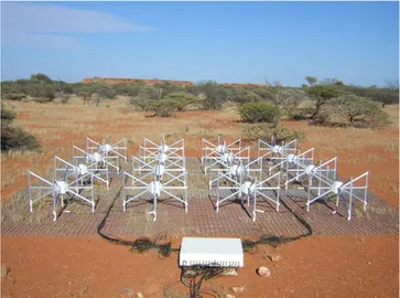
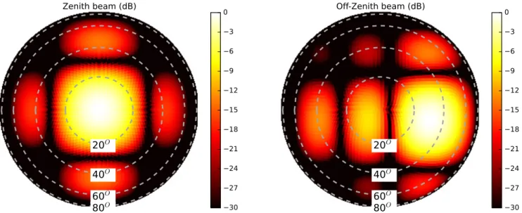
The MWA consists of 128 antenna elements positioned in a centrally concentrated, quasi-random distribution over a radius of 1.5 km. Each antenna element(MWA tile) is a 4×4 grid of dual-polarization bowtie dipoles with center-to-center spacing of 1.1 m (half-wavelength at 136 MHz) centered on a 5 m×5 m wire mesh ground screen (Figure 1). The signals from the 16 antennas(each with a dual-polarization low noise amplifier (LNA)) are summed in an analog beam-former with selectable delay lines, capable of applying phase gradients across the grid of dipoles to steer a beam of width full width at half max 25°/(ν/150 MHz) to elevations as low as 30°. We characterize the beam-former paths for delay bits 00000(0 ns) and 11111 (13 ns); the actual EOR delays corresponding to elevations above 60° are typically 5 ns or smaller, and thus, in between these two cases. Figure2 shows the zenith beam as well as a representative off-zenith beam. Thefirst field tests on an early version of the MWA tile were presented by Bowman et al.(2007), followed up by anechoic chamber measurements (Williams 2012) and satellite-based measurements (Neben et al.2015).
We characterize gain and group delay variation among the cables, LNAs, and beam-former signal paths that comprise an MWA tile through precision vector network analyzer (VNA) measurements of these components. We employ an experi-mental setup that mitigates the challenges generally faced by such low frequency RF measurements such as reflections at interfaces or due to cable bending, parasitic RF coupling, VNA noise, and saturation of analog components. We discuss uncertainty estimation and perform repeatability checks.
In addition, tilts and misalignments of the deployed MWA tiles contribute to antenna-to-antenna beam variation and concomitant beam mismodeling. We characterize these effects using the known MWA tile positions and elevations.
2.2. Gain and Group Delay Experiments
Gain and group delay measurements are conducted on LNAs, dipole cables, and beam-former paths using the setups described in more detail in the sections below. In all cases, we Figure 1. One of the 128 deployed MWA tiles in the Murchison Radio Observatory, Western Australia.
20
For instance, if two−20 dB reflections create a signal which adds π/2 out of phase with the main signal, a phase error of∼1deg is created, equivalent to a delay of 20 ps at 150 MHz.
perform measurements over the band 100–200 MHz, then retain the group delay and gain rms at 150 MHz for our beam-forming error budget; the rms is observed to be relatively frequency-independent over this band. Note that the physical gains and phases show some frequency dependence across this band, but only relative differences between the sixteen dipole pathways distort the beam pattern. The mean gain and group delay through the 16 signal paths are absorbed into each tileʼs calibration amplitude and phase. For the same reason, gains and group delays of the VNA and measurement cables are irrelevant.
We use an Anritsu MS2024A vector network analyzer set to low probe power(−30 dBm) and 30 trace averaging. The VNA is optimized for wide band (GHz) measurements, and we mitigate small-scale(sub MHz) systematics through binning to 16 MHz. In each of these windows, we average the gains measured at 0.36 MHz resolution, and compute the mean group delay by fitting a ramp to the measured phases. We perform repeated measurements on each component after disconnecting and reconnecting the entire measurement setup in order to estimate uncertainties due to slight bending of probe cables or imperfect cable connections.
2.2.1. LNA Measurements
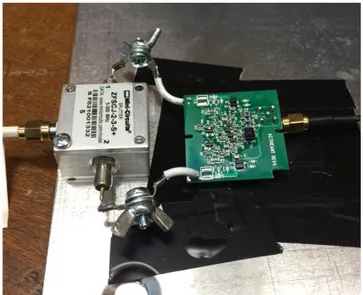
Precision LNA measurements are particularly challenging in a laboratory setting given their exposed leads, which, in a deployment environment, are fed balanced input by two dipole arms. Figure 3(a) shows a diagram of our solution. We use a 180° two-way power splitter (Mini-Circuits ZFSCJ-2-3-S+) to split the VNA probe signal into two balanced inputs to the LNA, both mounted above an aluminum plate to mitigate RF coupling (Figure 4). The aluminum plate is grounded to the splitter case, and then to the VNA probe cable shield. We fabricated angle connectors to secure the LNA leads to the center conductors of the power splitter outputs with as little exposed wire as possible. The LNA is powered through a Bias-T (Mini-Circuits ZFBT-4R2G-FT+) with a 5 VDC power supply.
We use this testing setup to characterize 16 single-polarization LNAs. Due to their different cable lead lengths,
the X and Y boards have systematically different group delays, which we correct for the subsequent analysis. As bending of these leads contributes to group delay variation among different LNAs, the LNA design was subsequently modified to fit both polarizations on the same circuit board and eliminate the excess lead cable. To approximate the level of group delay variation in these dual-polarization LNAs, we estimate the group delay variance contributed by the cable leads as equal to the measurement uncertainty (assumed to be dominated by cable lead bending), and subtract it from the total observed group delay variance for the single-polarization LNAs. Figure 5 shows our measured gains and group delays with measurement uncertainties of ±0.03 dB and ±15 ps through repeated measurements on the same set of LNAs. Measurements on different LNAs are slightly offset in frequency for ease of comparison. We observe significant (relative to measurement uncertainty) gain and group delay rms at 150 MHz of 21 ps and 0.09 dB, with the worst cases 2σ–3σ away from the mean. Subtracting(in quadrature) the 15 ps measurement uncertainty due to cable bending from the total delay rms yields an intrinsic LNA delay rms of 15 ps.
2.2.2. Cable Measurements
Figure 6 shows our dipole cable gain and group delay measurements relative to an average cable, with rms measure-ment errors of ±0.0093 dB and ±6.2 ps. At 150 MHz, we observe a significant (relative to the measurement error) group delay scatter of 34 ps rms and an insignificant gain scatter of 0.013 dB rms. Outliers are seen 2σ–3σ away from the mean. The dipoles cables are specified to be phase matched to ±1°–3° over 100–200 MHz. This translates into a group delay rms of ±19–55 ps, and is consistent with our measurements.
2.2.3. Beamformer Measurements
Gains and group delays of a set of 16 beam-former inputs for one polarization were measured in a testing setup depicted in Figure3(b). To avoid bending of the VNA probe cable when moving it across the 16 beam-former inputs, a dipole cable was used to connect the VNA probe cable to the desired beam-Figure 2. Ideal (no beam-forming errors) beams for a zenith pointing (left) and a representative off-zenith pointing (right) shown in sine-projection in units of dB at 150 MHz. The off-zenith beam is pointed at(θ, f)=(53°, 101°).
former input. Figure 7 shows our measured gains and group delays for the shortest delays on these 16 beam-former inputs with measurement uncertainties of 4.9 ps and 0.026 dB. We observe an rms of 21 ps and 0.4 dB at 150 MHz, with the worst cases 2σ–3σ from the mean. The longest delays through these beam-former inputs correspond to all delay lines (“bits”) engaged, yielding ∼13.5 ns of delay. We also probe the maximum delays through these beam-former inputs and find rms’ of 54 ps and 0.43 dB at 150 MHz.
2.3. Tile Tilts and Rotation
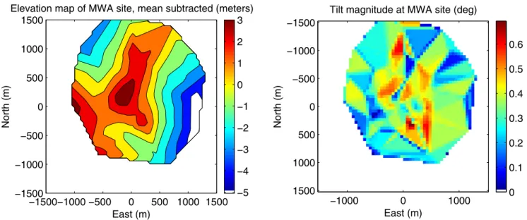
As the MWA was constructed around the apex of a slight hill to avoidflooding, a planar fit to the tile positions is quite poor. In principle tile tilts and rotations could be measured and incorporated into data reduction; however, this has not yet been done. In this paper, we conservatively incorporate them into our budget of antenna-to-antenna variation. We estimate tile tilts by gridding the differential GPS mapped tile positions, then compute the magnitude of the gradient. Using a 60 m grid spacing we find the rms of the tilt (away from zenith) magnitude to be 0°.27, with some tiles having tilts of up to 0°.4 (Figure8). These numbers are of the order of the precision of the differential GPS measurements used to determine the tile corners, so for simplicity we assume an rms of∼0°.3 for EW tilt, NS tilt, and rotation in subsequent simulations.
2.4. Budget of Beamforming Errors
We compile the measurements presented in this section into a budget of beam-forming errors in Table 1. Additionally we include the estimated dipole position precision of 0–17 ps estimated in Appendix A.3as it is comparable with the other sources of group delay scatter. Summing these group delay scatters in quadrature gives a total rms of 46 ps (68 ps) using the shortest(longest) beam-former delays. In contrast, the gain scatter is dominated by variation over the beam-former inputs of 0.4 dB for both delay settings. Lastly, overall tilts and rotations of the tile with 0°.3 rms are included separately. Figure 3. Diagram showing our LNA and beam-former testing setups (Section2.2.1). Note that LNA measurements are conducted above a ground plate to mitigate the effects of exposed antenna leads.
Figure 4. Photograph of the LNA ground plate setup depicted in Figure3and described in Section2.2.1.
Figure 5. Gain and group delay measurements on a set of 16 LNAs are shown relative to the mean LNA, as described in Section2.2.1. Error bars of±15 ps and ±0.035 dB are the rms of repeated measuerments. At 150 MHz, an rms of 22 ps and 0.092 dB is observed. The worst cases are observed 2σ–3σ away from the mean.
Figure 6. Gain and group delay measurements on a set of 10 dipole cables are shown relative to the mean cable, as described in Section2.2.2. Error bars of±6.2 ps and±0.0093 dB are the rms of repeated measurements. At 150 MHz, an rms of 34 ps and 0.013 dB is observed. The worst cases are observed 2σ–3σ away from the mean.
Figure 7. Gain and group delay measurements on the shortest delays of 16 beam-former inputs for one polarization are shown relative to the mean, as described in Section2.2.3. Error bars of±4.9 ps and ±0.026 dB are estimated from repeatability studies. At 150 MHz, an rms of 21 ps and 0.41 dB is observed. The worst cases are observed 2σ–3σ away from the mean.
3. SIMULATING BEAMS WITH BEAMFORMING ERRORS
We study the separate and cumulative effects of beam-forming errors on beam patterns through simulations using the budget presented in Section2.4, assuming that the dipole gain and delay errors and the tile tilts and rotations are randomly scattered around zero. We incorporate these errors into a simple analytic beam model and compute statistics on the set of slightly corrupted beams. Extensive numerical modeling (Sutinjo et al. 2014) shows slight corrections relative to the analytic model toward the edge of the main lobe and in the sidelobes, especially at higher frequencies toward 200 MHz, but is susceptible to beam-forming errors in largely the same way as the analytic beam.
The analytic electricfield beam, b(θ, f, λ), models the tile as a 4×4 grid of EW-oriented Hertzian dipoles above a perfect, infinite ground plane, with no mutual coupling,
b e A b , , 1 1 sin sin , , . 1 ih 4 cos 2 2 0 ( ) ( ) ( ) ( ) ( ) q f l q f q f l l = - -´ p ql
Here h=0.3 m is the dipole center height above the ground screen and division by b0(λ) normalizes the simulated beam to unity in the boresight direction of the ideal(no beam-forming errors) beam to simulate the effect of interferometric calibra-tion. The power beam is given by B(q f l, , )=∣ (b q f l, , )∣2.
A(θ, f, λ) is the array factor given gain errors {δGi} (dB), delay errors{δτi}, and pointing delays {τi}, defined as
k x A , , 10 exp i 2 if , 2 i G i i i 1 16 20 i (q f l)=
å
d ( · - p (t +dt)) ( ) =where k is the wavevector of the incoming radiation. During simulations in which the tile tilt and rotation are allowed to vary, horizontal coordinates θ (zenith angle) and f (azimuth, starting from the north, increasing toward the east) are replaced with coordinates from a tilted/rotated coordinate system.
For each of several possible systematics (σdelay=50 ps group delay errors, σtilt,rot=0°.3 tile tilt/rotation errors, and σgain=0.5 dB gain errors), we generate 128 tile realizations to represent the range of antenna beams in the MWA. We use the HEALPix pixelization of the sky (Górski et al. 2005) with nside= 32, corresponding to a resolution of 1°.8. This resolution is sufficient to resolve structure in the smooth beam pattern except within several degrees of the nulls. The effect of the ensemble of these slightly corrupted beams on science results depends on the type of analysis employed. In Section4 we consider the effects on power spectrum analyses, but we focus in this section on the effects on radio interferometric imaging. The effective beam of a naturally weighted image is the baseline-averaged beam,
B N b b , 1 , , . 3 i j i j baseline averaged baselines (q f)=
å
(q f) *(q f) ( ) -¹Note that while the voltage beam is in general complex, the baseline-averaged beam is real because both b bi j* and b bj i* are included in the sum.
We plot in Figure9 (left panel) the baseline-averaged beam relative to the ideal model for each systematic separately Figure 8. Map of the tilt magnitude of the MWA site computed by gridding the 3D tile positions and taking the gradient. Triangular features are artifacts from sparse grid coverage by the antenna positions; nonetheless their magnitudes are likely reasonable approximations, perhaps even underestimates of the land tilts given that small scale topographic structure is unconstrained.
Table 1
Beamforming Error Budget at 150 MHz
Systematic Name rms
Cable group delay 34 ps
LNA delay 15 ps
Beamformer delay(shortest delay) 21 ps Beamformer delay(longest delay) 54 ps
Dipole position 0–17 ps
Cable gain 0.013 dB
LNA gain 0.09 dB
Beamformer gain(shortest delay) 0.41 dB
Beamformer gain(longest delay) 0.43 dB
Tile tilt/rotation 0°.27
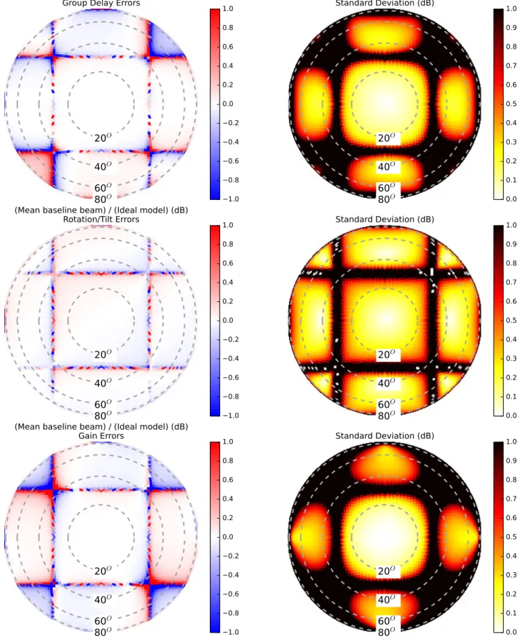
Figure 9. Baseline-averaged beam (left) and standard deviation (right) of simulated beams relative to the ideal model: σdelay=50 ps group delays (top), σtilt,rot=0°.3
(middle), and σgain=0.5 dB (bottom). Even though the individual beams exhibit fluctuations at the 0.2–0.5 dB level near the edge of the mean lobe and in the
sidelobes, the effects on the baseline-averaged beam are at the sub-percent level, except within several degrees of the sidelobes. This is due to partial cancellation of the complex beam errors when combining the complex pair-product beams of different visibilities, here calculated assuming natural weighting. The color scale in the right panel is saturated at 1 dB.
(delay, gain, and tilt/rotation errors), observing deviations only at the sub-percent level in the main lobe and sidelobes(though larger deviations are present within several degrees of the nulls). In the limit of infinitely many antennas these deviations would approach zero; but with only 128 antennas, these plots give a sense of the MWAʼs baseline-averaged beam. Beware that these sub-percent errors mask the fact that antenna-to-antenna variation will limit the accuracy of source deconvolu-tion. To quantify the level of antenna-to-antenna variation implied by our beam-forming error budget, we plot in the same figure (right panel) the standard deviation of the ratio of beam power response in each sky pixel to ideal beam power over the set of 128 simulated beams. The standard deviation is computed over this set of beam ratios in dB. We observe that individual beam realizations exhibitfluctuations at the level of 0.2–0.5 dB toward the edge of the main lobe (θ20°) and in the sidelobes with the tilt/rotation errors producing the smallest effects. The effects of the gain and delay errors appear similar in magnitude, and all exhibit largefluctuations near nulls where our dB standard deviation metric ceases to be meaningful.
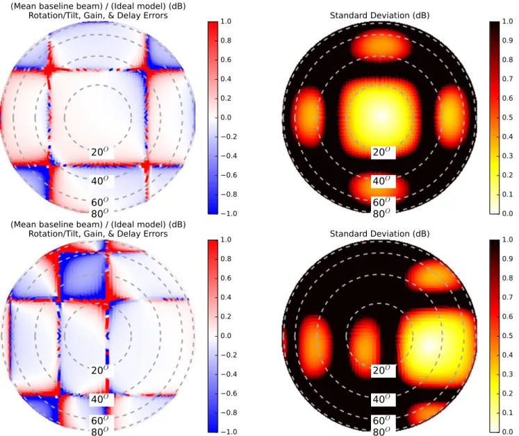
Next we simulate a beam with the entire realistic systematic budget (σdelay=50 ps, σgain=0.5 dB, and σtilt,rot=0°.3) for both the zenith pointing and the off-zenith pointing(Figure10). In aggregate, these errors manifest asfluctuations at the level of 0.5 dB near the edge of the mean lobe θ∼20°, and 0.5–0.75 dB (10%–20%) in the sidelobes, as seen in the standard deviation plots. We also plot three sample realizations (Figure11) of these corrupted beams relative to the ideal ones, which clarify the effects on individual tile beams. These realizations also illustrate the improvements which could be achieved through use of per-antenna complex primary beams in the analysis. The left column shows these beams relative to the ideal model on a compressed color scale highlighting the effects on the nulls. The bias within several degrees of the nulls is at the∼5–10 dB level, though these exact numbers depend somewhat on pixel size, as the beam is changing rapidly in these regions. Note that despite this consistent power bias, the random beam phases in these regions produce a baseline-averaged beam without such a bias(Figures 9,10). The right column shows these same ratio plots but with expanded color Figure 10. Baseline-averaged beam (left) and standard deviation (right) of simulated beams using the full beam-forming error budget (σdelay=50 ps group delays,
σtilt, rot=0°.3, and σgain=0.5 dB) for a zenith pointing (top) and the off-zenith pointing (bottom).
Figure 11. Each row shows a realization of a simulated beam relative to the ideal beam (in dB) on a compressed color scale (left) and on an expanded color scale (right). This simulation used the full beam-forming error budget of σdelay=50 ps, σgain=0.5 dB, σtilt,rot=0°.3. Here we see up and down fluctuations in the
scales highlighting the 0.5–1 dB level fluctuations seen in the main lobe and in sidelobes, a factor of a few larger than those observed in Figure10for each systematic individually. These fluctuations are unsurprisingly asymmetric, but appear coherent on the scale of a sidelobe.
Lastly, we consider in more detail the effects of beam-forming errors on the nulls near the main lobe and near the horizon. We first rerun our simulations with finer angular resolution of 0°.01 on a slice through the NS plane. We show the results in Figure12where we zoom in around thefirst null and near the horizon. We plot the ideal beam in black and our 128 realizations of beams with beam-forming errors in gray (both plotted as power beams), noting that in both regions the beam-forming errors “fill in” the analytically zero nulls and their surroundings so thefirst null bottoms out between roughly −55 and −30 dB, and the null at ∼85° bottoms out between −70 dB and −40 dB, vanishing entirely from some realiza-tions. However, cancellation of the complex errors in the simulated beams results in a baseline-averaged beam (Equa-tion(3)) which tracks much more closely with the ideal beam than any individual realization. This same effect is seen in the previousfigures. The deviations of the baseline-averaged beam away from the ideal beam are much smaller than those of individual antenna beams. The reason is that the baseline-averaged beam amounts to an average ofRe( (bi q f, )bj*(q f, )) over antennas i<j, and this can be negative near the nulls depending on gain and delay errors.
4. EFFECTS ON POWER SPECTRUM ANALYSES We present in this section a discussion and preliminary modeling of the effects of unmodeled primary beam variation among antenna elements in a 21 cm EOR power spectrum analysis. We focus on the effects for the MWA, but comment on other power spectrum analyses as well. A comprehensive quantitative evaluation of the effects of these errors in real
analysis pipelines demands detailed instrument simulations, building on those of Thyagarajan et al. (2015b) to take into account primary beam variation as in Shaw et al. (2015) and Asad et al.(2015). We leave this for future work, and consider here the qualitative effects of primary beam variation in interferometric calibration, the forming of image cubes, and power spectrum analysis. We supplement this qualitative discussion of the effects on a power spectrum analysis using the simple delay spectrum technique of Parsons et al.(2012a, 2012b) on a representative baseline.
4.1. Calibration and Forming Image Cubes
The MWA uses a sky model-based calibration scheme in which model visibilities are computed for a model sky distribution, and matched to the measured visibilities byfitting for antenna-based complex gains. Due to primary beam variation among the antenna elements, sources will appear with different amplitudes to different antennas, effectively adding a “noise” to measured visibilities relative to the ideal model. This noise adds to the inherent inaccuracy of the sky model. Given that such inaccuracies likely manifest most strongly from sources in the sidelobes where they are most difficult to measure, the resulting visibility errors rotate rapidly with time and frequency, suggesting time and frequency averaging of calibration solutions as a method to mitigate such sky-modeling errors (Braun 2013; N. Barry et al. 2016, in preparation). This approach will also mitigate sky-modeling errors due to primary beam variation, though it is unknown if time and frequency averaging alone will be sufficient to isolate foregrounds away from the 21 cm signal. Dillon et al. (2015) and A. P. Beardsley et al.(2016, in preparation) assume that all MWA antennas have the same bandpass up to low order polynomial corrections, further reducing both sky modeling errors and thermal noise. In any case the more immediate cause of calibration-induced frequency structure is miscalibration of Figure 12. We zoom in around the first null and near the horizon along a NS slice through the beam after running simulations with our full beam-forming errors budget with 0°.01 resolution. The nulls in all 128 beams with beam-forming errors ( b∣ ∣i2) (gray) are “filled in” by the errors; however, the baseline-averaged beam (Equation (3)) (red dashed) remains very close to the ideal power beam ( b∣ ∣2) (black) for the reasons discussed in Section3. This demonstrates that beam-forming
fluctuations of different antennas tend to average out in imaging. Still, the antenna-to-antenna variation will limit deconvolution accuracy.
2010; Williams et al. 2012; Bernardi et al.2013; Dillon et al. 2014, 2015). Antenna-to-antenna beam variation will disturb all these weighting steps, slightly upsetting the minimum-noise optimal weighting. Furthermore, as noted in Section3, though the mean imaging beam, and thus, the dirty apparent source fluxes, are nearly unaffected by the beam-forming errors due to cancellation of complex beam errors, the antenna-to-antenna variation will still limit deconvolution accuracy, and thus, foreground modeling accuracy. This is because beam-forming errors alter the apparent point-spread function because side-lobes from different visibilities now have slightly different weights which do not cancel out as they do at the exact source position. Further studies are needed to assess the effect in more detail, and quantify the deconvolution residuals.
4.2. Power Spectrum
A power spectrum analysis diverges from an imaging analysis by incoherently averaging fourier modes (to bin different k modes into a 1D power spectrum) instead of coherently averaging them. Thus even though the effects of beam-forming errors on the baseline-averaged beam are small as discussed above, further operating on the image to produce a power spectrum can make these errors very significant. Even assuming all antennas are perfectly calibrated despite the primary beam variation, sources will appear slightly brighter to some antennas and slightly dimmer to others. Subtraction of a foreground model which neglects this effect by assuming ideal beam patterns leaves residuals which vary over this spherical shell, and do not average down in the incoherent power average.
It is these effects, as opposed to calibration effects, which we expect to be the most significant in power spectrum analysis, and to further quantify them, we simulate a power spectrum on a single baseline with and without unmodeled beam-forming errors. In essence, we ask what errors would we make in a power spectrum analysis if we knew the foregrounds perfectly but lacked measurements of the exact antenna-to-antenna variation. We consider their implications for two different foreground mitigation strategies: foreground subtraction and foreground avoidance. Our simulations are centered on the MWA “EOR0” deep integration field, centered at R.A. (J2000)=0h0m0s and decl.(J2000)=−30° 0′ 0″, and the sky is modeled as the sum of a deep MWA point source survey within 20° of the field center (P. Carroll et al. 2016, in preparation), the shallower but wider MWA commissioning point source survey(Hurley-Walker et al.2014), the Culgoora
tilt/rotation errors, because as Section 3 suggests, they are subdominant to gain and delay errors.
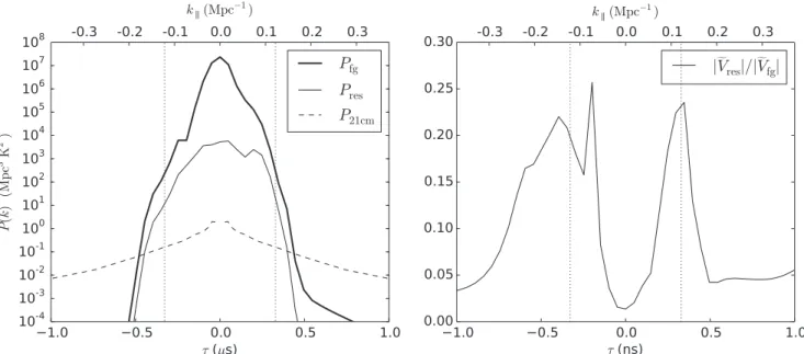
We plot in the left panel of Figure13the mean foreground power spectrum computed from 100 realizations of simulated visibilities with beam-forming errors, Pfg, and then the power spectrum after subtracting ideal model visibilities, Pres. The delay power spectrum is computed as outlined by Thyagarajan et al. (2015b) using a Blackman–Harris Window function (Parsons et al.2012a,2012b). The sky power (thick black line) dominates over the cosmological signal by typically 4–7 orders of magnitude in power within this baselineʼs horizon limits (the well-known foreground “wedge”; Datta et al. 2010; Morales et al. 2012; Trott et al. 2012; Vedantham et al. 2012; Pober et al. 2013; Thyagarajan et al. 2013; Dillon et al. 2014; Liu et al.2014a,2014b), but quickly drops below the cosmological signal(dashed line) (Mesinger et al.2011) outside these limits (in the the “EOR window”). This demonstrates the “foreground avoidance” approach and shows that it reveals the cosmological signal even in the presence of frequency dependent beam-forming errors. Measurement of the cosmological signal within the baselineʼs horizon limits, where it is largest, requires model subtraction with 2–4 orders of magnitude more dynamic range than is achieved by neglecting beam-forming errors in the foreground model(thin black line). Note that Thyagarajan et al. (2015a, 2015b) observe that an increased near-horizon beam response relative to our analytic tile model tends to add a power bump at the baselineʼs horizon limits (the outer prongs of their “pitchfork”).
To be sure, these residuals due to beam errors will average down somewhat when different baselines are coherently averaged in the same k cell, but 104–108independent samples would be needed to bring them below the level of the EOR. The maximum number of independent samples is the number of antennas in the array, each with a different realization of beam-forming errors. We thus see that the coherent averaging down of beam errors in imaging power spectra is only a small effect.
To better understand these results, we plot in the right panel of Figure13 the residual of the simulated visibilities in delay space relative to those without beam-forming errors V∣res V ,fg∣
where V represents the frequency fourier transform of V(f). As expected, the fractional residuals are largest (∼20%) near the delays corresponding to the baselineʼs horizon limit (300 ns), as these delays correspond to very low points in the beam where the effects of the beam-forming errors are largest. At zero delay, corresponding to emission from the plane bisecting the
baseline vector and containing zenith, the fractional residual is much lower(1.5%). This highlights again that beam modeling errors affect preferentially the weakest beam regions which, because they are closest to the horizon, are most at risk of leaking power into the EOR window.
5. DISCUSSION
Efforts to detect neutral hydrogen emission at cosmological distances in the presence of bright galactic and extragalactic foregrounds are drawing attention to radio astronomy systema-tics, in particular primary beam characterization. Following up on efforts to constrain the mean MWA tile beam through advanced modeling (Sutinjo et al. 2014) and measurements (Neben et al. 2015), we explore the next order effect of antenna-to-antenna variation. We establish a budget of relevant beam-forming errors and run simulations drawing from this distribution to study the effects on beam patterns.
We characterize the beam-former paths, dipole cables, and LNAs used in the MWA tile through laboratory experiments. Summing in quadrature the group delay errors of the cables, the LNAs, and the beam-former paths, we find 46 ps of group delay rms, and 67 ps when using the longest beam-former paths instead. This level is roughly 10% of the beam-former shortest delay of 435 ps. Gain errors appear dominated by 0.5 dB rms among the beam-former inputs. These errors, in addition to tile tilt/rotation errors at the ∼0°.3 level will vary from tile to tile, yielding visibility errors that do not average down with time.
We run simulations drawing from these gain, delay, and alignment errors to study the magnitude and angular-depen-dence of the resulting beam errors. None of these systematics is observed to have more than a percent effect on the baseline-averaged beam(the effective beam of an image) except within several degrees of the nulls. In contrast, power spectrum
measurements are more sensitive to the beam standard deviations, essentially the typical tile-to-tile variation as a function of angle on the sky. Standard deviations of roughly 0.5–0.75 dB (10%–20%) are observed toward the edges of the main lobe (20°<θ<40°) and in the sidelobes when all systematics are included(Figure10).
To study the effects of these beam-forming errors on 21 cm power spectrum analyses, we break down such an analysis into the different steps where beam-forming errors could affect the results, and qualitatively evaluate their likely severity. They will limit calibration fidelity, though averaging in time, frequency, and over antennas can mitigate them to some extent. While the effect on the effective imaging beam will be small due to the cancellation of complex visibility errors in imaging (due to coherent combination of fourier modes), antenna-to-antenna variation will limit deconvolution accuracy nonetheless. By the same token, the effects in the power spectrum space will be larger, as here different fourier modes are added incoherently, binning fourier modes into a 2D or 1D power spectrum.
We confirm this with a simple simulation of the delay spectrum of a single visibility, addressing the question of what errors we would make in a power spectrum analysis if we knew the foregrounds perfectly but lacked measurements of the antenna-to-antenna beam variation. We find that unmodeled beam-forming errors are severe enough to make foreground subtraction impossible within the baselineʼs horizon limits (in the wedge), where per-antenna primary beams will be necessary. However, even including an overestimate of their frequency dependence, the beam-forming errors do not leak significant frequency structure into “the EOR window” which remains nearly clear of foreground contamination. Thus the foreground avoidance approach being pursued by PAPER, the Figure 13. We simulate delay power spectra for a single baseline at 150 MHz (z∼8.5) using the Global Sky Model and point source catalogs with and without beam-forming errors(dipole gain and delay errors of rms 0.5 dB and 50 ps and delay slope errors of rms 5 ps/MHz). We use a bandwidth of 20 MHz and a Blackman– Harris window function. Left: the total foreground power Pfg(thick black line) is predominantly contained within this baselineʼs horizon limits (vertical dotted lines)
where it dominates over the cosmological signal, but falls rapidly below that signal just outside the horizon limits(the “EOR window”). This demonstrates that the “foreground avoidance” approach reveals the cosmological signal even in the presence of frequency dependent beam-forming errors. Measurement of the cosmological signal within the baselineʼs horizon limits, where it is largest, requires model subtraction with 3–4 orders of magnitude more dynamic range in power than is achieved by subtracting an otherwise perfect foreground model with unmodeled beam-forming errors Pres(thin black line). Right: the fractional visibility
residual V∣ resVfg∣ after subtraction is largest near the baselineʼs horizon limits (corresponding to large zenith angles near the horizon, where the effects of beam-forming
errors are largest, and lowest at zero delay(in the plane bisecting the baseline and including zenith).
the cosmological signal using zenith-tracking dishes rather than phased arrays, and foreground avoidance rather than the more challenging subtraction. In contrast, observatories relying both on beam-forming and foreground subtraction (e.g., LOFAR and SKA-Low) must model the sky and primary beams (either through calibration or measurement) to four to five orders of magnitude of dynamic range lest foreground residuals swamp the feeble cosmological signal.
This work was supported by NSF grant AST-0821321, the Marble Astrophysics Fund, and the MIT School of Science. We thank Aaron Ewall-Wice and Hamdi Mani for assistance in running these experiments, Steve Burns for debugging beam-former issues, and Danny Jacobs, Nithyanandan Thyagarajan, and Lu Feng for helpful discussions.
This scientific work makes use of the Murchison Radio-astronomy Observatory, operated by CSIRO. We acknowledge the Wajarri Yamatji people as the traditional owners of the Observatory site. Support for the MWA comes from the U.S. National Science Foundation (grants AST-0457585, PHY-0835713, CAREER-0847753, and AST-0908884), the Aus-tralian Research Council (LIEF grants LE0775621 and LE0882938), the U.S. Air Force Office of Scientific Research (grant FA9550-0510247), and the Centre for All-sky Astro-physics (an Australian Research Council Centre of Excellence funded by grant CE110001020). Support is also provided by the Smithsonian Astrophysical Observatory, the MIT School of Science, the Raman Research Institute, the Australian National University, and the Victoria University of Wellington(via grant MED-E1799 from the New Zealand Ministry of Economic Development and an IBM Shared University Research Grant). The Australian Federal government provides additional support via the Commonwealth Scientific and Industrial Research Organisation (CSIRO), National Collaborative Research Infra-structure Strategy, Education Investment Fund, and the Australia India Strategic Research Fund, and Astronomy Australia Limited, under contract to Curtin University. We acknowledge the iVEC Petabyte Data Store, the Initiative in Innovative Computing and the CUDA Center for Excellence sponsored by NVIDIA at Harvard University, and the International Centre for Radio Astronomy Research(ICRAR), a Joint Venture of Curtin University and The University of Western Australia, funded by the Western Australian State government.
ments as follows. The desired frequency band represents an order unity fractional bandwidth, necessitating a wideband antenna with a smooth frequency response. In particular, significant frequency structure on scales smaller than the nominal power spectrum analysis bandwidth of 10 MHz(set by timescale of Δz∼0.5 over which the cosmological signal is expected to evolve) would complicate beam modeling and risk smearing smooth spectrum foregrounds into spectrally noisy signal-like modes. A largefield of view, in comparison to more traditional radio telescopes like the Very Large Array, is also desired to maximize the cosmological volume over which to measure the EOR power spectrum. Instrumental noise is minimized to the sky noise limit through use of LNAs placed as early in the signal chain as possible. A steerable beam was also desired to allow deep observing on discrete patches of sky, and thus coherent integration on power spectrum modes. This strategy reduces noise much more quickly with integration time at the expense of an increase in cosmic variance noise (Trott 2014). Lastly, and arguably most importantly, is the large required collecting area at modest cost, achieved with an array of the order of one hundred low cost ($2500/ea) antenna elements. The MWA is a realization of the“Large N– Small D” array concept consisting of a large number of small diameter antenna elements made possible by advances in parallel computer processing.
Though it is tuned to some extent to achieve the high surface brightness sensitivity required by EOR science, this design also permits a host of other low frequency science ranging from transient searches and source surveys to solar and ionospheric science (Bowman et al. 2013). The MWA tile design is, therefore, a compromise to meet different science goals. Further optimization for EOR science is possible, for example, HERA, is pursuing larger antenna elements to increase sensitivity without extra computing cost. At the array level, the HERA antennas will be positioned on a regular grid to achieve many redundant baselines, and thus allow coherent integration on individual power spectrum modes.
A.2. Dipole Element
Each MWA dipole element is a set of two orthogonally crossed vertical bowties, each of length 74 cm and height 38 cm. Each bowtie is composed of two aluminum arms mounted at a PVC hub such that the lowest part of the antenna is 8 cm above the ground screen. In principle, an infinite bowtie antenna has infinitely broad bandwidth because it has no characteristic length scale. A real bowtie is truncated, which
introduces length scales and resonances, but the bandwidth remains broad and the response generally smooth on frequency scales of interest.
Note that despite the arms not being composed of solid metal sheets, the electrical performance of our bowtie differs negligibly from that of a more costly solid one while also mitigating wind loading. Other dipole style antennas were modeled in various orientations, but the bowtie was chosen for its relatively smooth gain over frequency, minimum gain variation over elevation, low horizon gain, absence of blind spots or other anomalies in the patterns or impedance, and impedance match with the LNAs.
One unexpected discovery was made during early antenna testing relating to coupling between adjacent dipoles in a tile. Interactions between the vertical pieces in a row or column of dipoles direct power toward the horizon in much the same way that one attaches perpendicular arms to a metal rod to form a directive Yagi antenna. Consequently, the dimensions of the antenna were adjusted to the present values to move this resonance to 240 MHz, near an already unusable satellite band. Inside each PVC hub is a dual-polarization LNA that also serves as a balun between the balanced bowtie terminals and the 50Ω coaxial cable to the beam-former. In detail, there is an amplifier on each of the four dipole arms. The amplified signals from opposing arms are combined through a center-tapped transformer balun to feed a 50Ω unbalanced coaxial cable.The LNA gain with a 50Ω source is ∼19 dB at 150 MHz. The impedance match with the sky is sufficient to make the system sky noise dominated. Quality control data on thefield-deployed dipole LNAs is collected periodically in an array dipole testing mode during which the beam-former paths are all switched off, then each is switched on individually. The LNAs are powered with a 5 V DC bias provided by the beam-former on the 7 m LMR-100 cables(50Ω), which also carry the sky signals in the opposite direction. In their deployed configuration, these cables arefixed with wire ties atop the ground screen.
A.3. Ground Screen
The 5 m×5 m ground screen is formed by three overlapped 2 m×5 m mesh panels welded together and laid directly on the ground. Each panel is constructed of 3.15 mm galvanized steel wire, welded together to form a grid of 50 mm×50 mm squares. Typical dipole position errors are at the 5 mm level or smaller on average throughout the dipole grid, due to mesh thickness and distortions due to handling, and also slightly larger errors overlapping the different mesh panels. Such horizontal errors are irrelevant for radiation incident from
zenith, but contribute per-dipole delays up to an rms of approximately 17 ps toward the horizon due to the altered light travel time to the different elements. In any case, these errors are subdominant to other errors discussed below.
No large or small scale ground leveling was attempted, but the flatness and alignment estimated with differential-GPS measurements is better than a few cm vertically and ∼1° in alignment with north and zenith. We discuss this alignment precision in more detail in Section 2. An electrical path to ground is provided through a connection to the wire chassis of the beam-former and subsequently to the receiver, itself grounded to metal ground stakes.
A.4. Beamformer
The beam-former contains two vertically offset delayline boards, one for each polarization, each fed by 16 dipole inputs. Each input is directed through a series of digitally switchable delay lines before being summed with the others with specified relative delays applied, and output to the receiver. Figure14 shows a block diagram of the signal path. Each input passes through a 4-pole lowpassfilter with a 3 dB cutoff at 600 MHz, a 30 dB amplifier, five sequential switched delaylines, a switch that either passes the signal or terminates with 50Ω, and lastly a cascade of two-way power combiners which sum the 16 inputs. Note that this low passfilter serves simply to protect the analog components from saturation; there is a second low pass anti-aliasingfilter in the receiver. The shortest delay line is 435 ps, a number determined by the requirement that the beam be steerable to 30° elevation with five delay line “bits” whose electrical lengths form a geometric series with a ratio of 2. These boards are also capable of applying Walsh switching to the summed signal to mitigate cross-coupling between different signal paths from different MWA tiles, though this feature has not been found to be necessary and has not been implemented. Digital communication to the beam-former to activate delay bits on each of the delay lines is transmitted in a “data over coax” configuration, multiplexed on the two RG-6 cables carrying the dual-polarization beam-former output to the receiver.
REFERENCES
Asad, K. M. B., Koopmans, L. V. E., Jelić, V., et al. 2015,MNRAS,451, 3709 Backer, D. C., Aguirre, J., Bowman, J. D., et al. 2009, in US Astro2010 Decadal Survey“Cosmology and Fundamental Physics” Science Frontier Panel
Beardsley, A. P., Hazelton, B. J., Morales, M. F., et al. 2013,MNRAS,429, L5 Bernardi, G., Greenhill, L. J., Mitchell, D. A., et al. 2013,ApJ,771, 105 Figure 14. For each polarization, each of 16 dipole signals passes through a balun/LNA (represented by the first amplifier in the diagram) mounted in the dipole hub with a gain varying between 16 and 25 dB across the band. The signal is then carried into the beam-former, where it goes through a low passfilter, an amplifier, five switchable delay lines, a series of two-way power combiners which sums the 16 dipole signals, then two more amplifiers. The delay lines are replaced by matching attenuators when disengaged. Walsh switching may be implemented directly after the power combiners. Driving just one beam-former input, the gain totals roughly 33 dB at 150 MHz accounting for losses in the power combiners and other components.
Liu, A., Parsons, A. R., & Trott, C. M. 2014b,PhRvD,90, 023019 Liu, A., Tegmark, M., Morrison, S., Lutomirski, A., & Zaldarriaga, M. 2010,
MNRAS,408, 1029
Loeb, A., & Furlanetto, S. R. 2013, The First Galaxies in the Universe (Princeton, NJ: Princeton Univ. Press)
Lonsdale, C. J., Cappallo, R. J., Morales, M. F., et al. 2009, Proc. IEEE, 97, 1497
Mesinger, A., Furlanetto, S., & Cen, R. 2011,MNRAS,411, 955 Mitchell, D., Greenhill, L., Wayth, R., et al. 2008,ISTSP,2, 707
Moore, D. F., Aguirre, J. E., Parsons, A. R., Jacobs, D. C., & Pober, J. C. 2013,
ApJ,769, 154
Morales, M. F., Hazelton, B., Sullivan, I., & Beardsley, A. 2012,ApJ,752, 137 Morales, M. F., & Matejek, M. 2009,MNRAS,400, 1814
Morales, M. F., & Wyithe, J. S. B. 2010,ARA&A,48, 127
Neben, A. R., Bradley, R. F., Hewitt, J. N., et al. 2015,RaSc,50, 614 Neben, A. R., Hewitt, J. N., Bradley, R. F., et al. 2016, ApJ, submitted
(arXiv:1602.05249)
Thyagarajan, N., Jacobs, D. C., Bowman, J. D., et al. 2015b,ApJ,804, 14 Thyagarajan, N., Udaya, S. N., Subrahmanyan, R., et al. 2013,ApJ,776, 6 Tingay, S. J., Goeke, R., Bowman, J. D., et al. 2013,PASA,30, e007 Trott, C. M. 2014,PASA,31, 26
Trott, C. M., Wayth, R. B., & Tingay, S. J. 2012,ApJ,757, 101
van Haarlem, M. P., Wise, M. W., Gunst, A. W., et al. 2013,A&A,556, A2 Vedantham, H., Udaya Shankar, N., & Subrahmanyan, R. 2012, ApJ,
745, 176
Virone, G., Paonessa, F., Peverini, O., et al. 2014, in IEEE Conf. Antenna Measurements Applications(CAMA), 1
Williams, C. L. 2012, PhD thesis, Massachusetts Institute of Technology Williams, C. L., Hewitt, J. N., Levine, A. M., et al. 2012,ApJ,755, 47 Yatawatta, S., de Bruyn, A. G., Brentjens, M. A., et al. 2013,A&A, 550,
A136
Zaroubi, S. 2013, in The First Galaxies, Vol. 396, ed. T. Wiklind, B. Mobasher, & V. Bromm(Berlin: Springer)