Approximation of the transient joint queue-length distribution in tandem networks

Approximation of the Transient Joint

Queue-Length Distribution in Tandem Networks

by

Jana H. Yamani

B.S Computer Science and Mathematics

Northeastern University, 2009

Submitted to the School of Engineering

in partial fulfillment of the requirements for the degree of

Master of Science in Computation for Design and Optimization

at the

MASSACHUSETTS INSTITUTE OF TECHNOLOGY

September 2013

0 Jana Yamani 2013. All rights reserved.

The author hereby grants to MIT permission to reproduce and to distribute

publicly paper and electronic copies of this thesis document in whole or in

part to any medium now known or hereafter created.

r I

Author ...

Certified by ...

Accepted by . .

..

. . . .

. . . . .

The

School of Engineering

n

August 15,2013

. . ... . . . . . . . . . . . . .

Carolina Osorio

Assistant Professor of Civil and Environmental Engineering

_1-

T

Thesis Supervisor

. . . . . .. . . .

Nicolas Hadjiconstatinou

Professo of Mechanical Engineering

Director, Computation for Design and Optimization (CDO)

Approximation of the Transient Joint Queue-Length

Distribution in Tandem Networks

by

Jana H. Yamani

Submitted to the School of Engineering in August 26, 2013, in partial fulfillment of the

requirements for the degree of

Master of Science in Computation for Design and Optimization

Abstract

This work considers an urban traffic network, and represents it as a Markovian queueing network. This work proposes an analytical approximation of the time-dependent joint queue-length distribution of the network. The challenge is to provide an accurate

analytical description of between and within queue (i.e. link) dynamics, while deriving a tractable approach. In order to achieve this, we use an aggregate description of queue

states (i.e. state space reduction). These are referred to as aggregate (queue-length) distributions. This reduces the dimensionality of the joint distribution.

The proposed method is formulated over three different stages: we approximate the time-dependent aggregate distribution of 1) a single queue, 2) a tandem 3-queue network, 3) a tandem network of arbitrary size. The third stage decomposes the network into

overlapping 3-queue sub-networks. The methods are validated versus simulation results. We then use the proposed tandem network model to solve an urban traffic signal control problem, and analyze the added value of accounting for time-dependent between queue dependency in traffic management problems for congested urban networks.

Thesis Supervisor: Carolina Osorio

Acknowledgements

This work was completed under the supervision of my research advisor, Professor Carolina Osorio. Carolina, an enormous thank you goes to you for believing in me, for encouraging me to take on new challenges every step of the way and for taking me in late and making it possible for me to complete this thesis in less than a year. I hope to always be in touch.

To my husband, Abdulrahman Tarabzouni: A special thank you goes to you for

encouraging me to come to MIT even when you knew you were going to be thousands of miles away from Leen and I. Your constant support, love and encouragement are what helped me overcome obstacles.

To my daughter, Leen Tarabzouni: You are my star. Thank you for reminding me that family is the most important thing, and for forcing me to take breaks from studying! It was great seeing you grow to be this wonderful positive person that you are today. It was great sharing the MIT journey with you. I hope one day you will go through it yourself. To my parents, siblings and in-laws: Thank you for your support and encouragement in tough times, and for reminding me that having my dreams met is something that I should work so hard for.

To the CDO administrator, Barbara Lechner: Thank you for being there when I needed you. You were always helping me get through academic and personal hardships. I wouldn't have done it without your constant support. You've been extremely missed. May you rest in peace.

To all my fellow friends at CDO: You have made my stay at MIT a memorable one. Thanks to each one of you. I hope to be in touch always.

To my fellowship sponsor, King Abdullah of Saudi Arabia, the Ministry of higher education and the Saudi Arabian Cultural Mission: thank you for your generous help and support. I am lucky to come from a country that supports education in all possible ways.

Contents

Cover page 1 Abstract 3 Acknowledgements 5 Contents 7 List of figures 9 List of tables 11 Chapter 1. Introduction 13 1.1 Literature review ... . 14 1.2 M odel background ... 18 1.3 O verview ... 19

Chapter 2. Model formulation 21 2.1 Aggregation-disaggregation framework ... 21

2.2 Aggregate transient model for a single and a network of tandem queues.25 2.2.1 Aggregate transient model for a single queue ... 25

2.2.2 Aggregate transient model for a three-queue tandem network ... 33

2.2.3 Aggregate transient model for an M-queue tandem network .... 46

Chapter 3. Validation 61 3.1 Single queue ... 62

3.2 Three-queue tandem network... 68

3.3 M-queue tandem network... .73

3.3.1 Five queue network ... .73

3.3.2 Eight queue network... .74

3.3.3 Twenty-five queue network .... . ... 77

Chapter 4. Case study 79 4.1 N etw ork... .79

4.2 Problem formulation... 81

4.2 Implementation notes ... 84

4.4 Results ... 85

4.4.2 High demand scenario ... 86

Chapter 5. Conclusion 89

Appendix 91

A Transition rate matrix for a three queue network... .91

List of

figures

2-1 Aggregating the state space of a single queue to three aggregate states ... 23

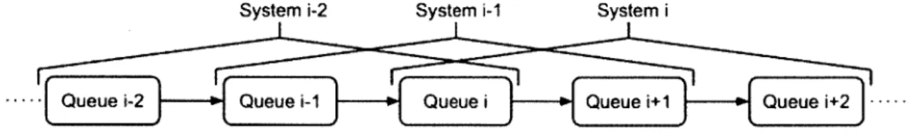
2-2 Decomposing the network to overlapping sub-networks of three queues .... 46

3-1 Results 3-2 Results 3-3 Results 3-4 Results 3-5 Results 3-6 Results 3-7 Results 3-8 Results 3-9 Results 3-10 Results 3-11 Results 3-12 Results 3-13 Results 3-14 Results 3-15 Results 3-16 Results 3-17 Results 3-18 3-19 3-20 of of of of of of of of of of of of of of of of of Histogram Histogram Histogram experiment experiment experiment experiment experiment experiment experiment experiment experiment experiment experiment experiment experiment the the the the of of of 1 at t=1,10,50 and error plots ... 63

2 at t=1,10,50 and error plots ... 64

3 at t=1,10,50 and error plots ... 64

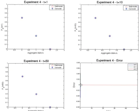
4 at t=1,10, 50 and error plots ... 65

5 at t=1,10, 50 and error plots ... 65

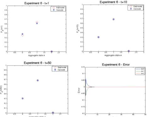
6 at t=l ,10, 50and error plots... 66

7 at t=1,10, 50 and error plots ... 66

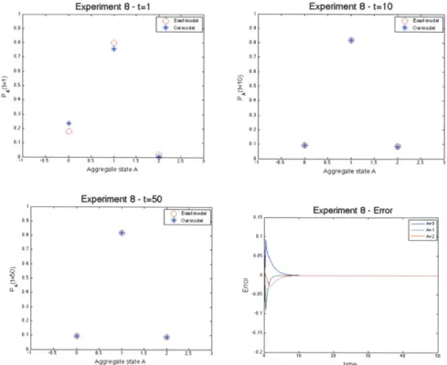
8 at t= I,10, 50and error plots... 67

9 at t=1 ,J0, 50 and error plots ... 67

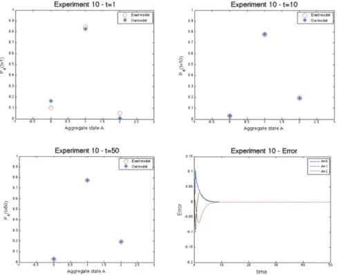
10 at t=1,10, 50and error plots... 68

1,2,3 for the 3 joint queue-length distribution ... 70

4,5,6 for the 3 joint queue-length distribution ... 71

7,8,9 for the 3 joint queue-length distribution ... 72

5-queue tandem 8-queue tandem 8-queue tandem 8-queue tandem network network network network experiment ... 74 experiment at t=1 ... 75 experiment at t=10... 76 experiment at t=50... 76

the 25-queue tandem network experiment the 25-queue tandem network experiment the 25-queue tandem network experiment errors errors errors at at at t=1... ..77 t=10... 78 t=50... 78

Urban road network of single roads for the case study ... 80

CDF's of the average trip time for the medium demand test ... 86

CDF's of the average trip time for the high demand test ... .87

4-1 4-2 4-2

List of tables

2-1 All blocking scenarios with their detailed information... 35

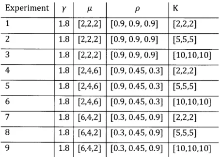
3-1 Experiments to test a single queue ... ... 63

3-2 Experiments to test a three-queue network... 69

3-3 Experiment to test a 5 queue tandem network ... 73

3-4 Experiment to test an 8-queue tandem network... ... .75

Chapter 1. Introduction

In urban traffic networks, to reduce congestion and improve network-wide performance, one must understand two aspects of the network: the dynamics within each link (i.e., road), and the possibilities of blockings to occur and propagate over time. Blocking occurs when a customer completes service in a link but cannot proceed downstream because the downstream link is full. Queueing theory helps in analyzing both aspects of the network by modeling links as queues. One can study the behavior of queues over time if the arrival process of customers and service mechanism are known. In this thesis, we will represent an urban road network as a Markovian finite capacity queueing network. We are interested in understanding the distribution of customers in the network at any point in time, which can be done through the analysis of the transient joint queue-length distribution (denoted transient joint distribution hereafter) of the network. Calculating the exact transient joint distribution is a computationally expensive task given the high dimensional system of differential equations to be solved; hence, the objective of this thesis is to analytically approximate the transient joint queue-length distribution of the network.

We will specifically look at M/M/I/K queues. The number of customers in an M/M/l/K queue is defined as a stochastic process, its state space is the set {0,1,2...,K}, where K is the state capacity of the queue. This type of queue is governed by independent identically distributed (iid) exponential interarrival times with arrival rate A and iid exponential service times with service rate pt. M/M/1/K queues are the most elementary of finite capacity queueing models (Strugul, 2000). They are also appealing to study because of the availability of closed-form expressions that describe a wide range of queue metrics.

1.2 Literature review

Calculating the exact transient queue-length distribution of a network requires working with exponentials of high-dimensional matrices that are computationally expensive to compute. Due to the mathematical difficulty of computing the transient distribution of a network, researchers have previously focused on developing models that calculate the steady-state distribution instead of the transient distribution (Phillips, 1995). In cases where there is a need to understand the transient distribution of the network before it reaches to steady-state or when the system does not reach a steady state, the transient

solution accurately portrays the behavior of the system as opposed to the stationary which if exists showcases only the final state of the network (Kaczynski, Leemis and Drew, 2012).

Although the literature focuses on steady-state queueing models (Phillips, 1995), transient queueing models have been studied and developed by researchers. In this

section, we will focus our investigation on models that look at finite capacity queues and yield expressions for the transient queue-length distributions for a single queue or a network of queues. These models are generally classified into three groups: exact models,

analytical approximation models, and numerical approximation models.

The first exact closed-form expression to the transient queue-length distribution of an MIM/l/K queue was developed by Morse (1958, p.65-67). Morse's closed-form equation expresses the transient distribution as the sum of the steady state solution and a transient term. As time increases in the network, the transient term becomes negligible compared to the steady-state solution. The transient solution given by Morse, while useful for a single queue, does not allow us to model a joint queue-length distribution of multiple queues. Takacs (1961) also derived a closed form that yields the same results as Morse

Another exact model is one developed by Parthasarathy (1987), which derives a transient expression for a single M/M/1/K queues that include integrals of Bessel functions. With small modifications, the expression given can be applied to different types of queues including single or multiple server queues, and queues with or without balking. For instance, Abou-El-Ata (1993) extended Parthasarathy's work to solve the transient behavior of an M/M/1/K queue with balking customers. Despite the fact that the transient expression can be applied to different queue types, the integrals of Bessel functions are complex and hard to accurately compute since they are defined as an infinite series. Given the above, exact models have certain limitations and complexities that can be overcome by approximate models.

When it comes to analytical approximation models, Stem's (1979) model for a single M/M/l queue uses the form of the queue-length distribution of the exact model in his approximation. The transient queue-length distribution is then expressed as a sum of exponential terms. The expression of the transient is then transformed to a form where the eigenvalues and vectors of the expression is used. Stem shows that the expression for the marginal distribution is in a form that lends itself to simple approximation for the transient mean queue-length. Not only does this method apply for a single queue, a

similar approach can be taken to obtain an approximation for the joint distribution of a network of queues. While this model seems to work well for any degree of accuracy, it is crucial to use a small time-step when computing the queue-length distributions, which would result in longer running periods.

Filipiak's (1988) model is another example of an analytical approximation model for calculating the transient queue-length distribution of a single M/M//K queue. The model is called a fluid flow approximation because the core of the model consists of differential equations describing the rate of flow of customers into and out of the queue and relating it to the transient distribution of the queue (Phillips, 1995). The differential equations contain some characteristic functions that if their roots were found, yield the transient distribution for the M/M/l/K queue.

Filipiak's method was then extended by Phillips (1995). Phillips' method however uses different characteristic functions that are easier to solve roots for. Either way, solving roots of high degree polynomials are usually expensive and time-consuming to compute.

Apart from analytical approximation models, numerical approximation models have also been developed to evaluate the transient queue-length distribution. These methods, however, deal directly with the differential equations of the queue-length distributions, which in most cases are high-dimensional systems to solve (Rothkopf and Oren, 1979). Grassmann's paper (1977), for instance, explores three different numerical methods to solve the transient queue-length distribution of M/M/l/K queues. The three methods are: Rung-Kutta, Modified Runge-Kutta and Liou, and Randomization. The methods are closely related, yet the randomization method is shown to be superior than the others. An important trait that these methods exploit is that they preserve the sparsity of the

transition rate matrix. It is also important to note that these methods can be applied to solve the queue-length distribution of a single Markovian queue or the joint queue-length distribution of a network of Markovian queues.

Despite the fact that numerical methods have very low execution time compared to exact and analytical approximation methods, the main problem faced by many authors is the high dimensional system of differential equations being solved. A queueing system with n queues leads to n-tuple states. There is then

HY=

1 Ki different states, where Ki is the capacity of queue i. The transition rate matrix will then be of dimension

(17W.=₁ Ki)2_{. Even for small values of Ki and n, this number can be very large and very} hard to store (Grassmann, 1977).

Dealing with a network with large numbers of queues or large queue capacities have been found challenging for many of the methods above. One way to reduce the dimensions of the system of equations being solved is by aggregating the queue-length state space. The aggregation process is done by combining some states into an aggregate states.

Aggregation of queue states for stationary Markov chain was introduced by Takahashi

derivation of a marginal aggregate length distribution and a joint aggregate queue-length distribution (Takahashi and Song, 1991). In Takahashi and Song's paper (1991), they enhanced the aggregation model by modeling the joint queue-length distribution of adjacent queues, therefore accounting for any blockings between queues. They showed an example of approximating the stationary distribution for a 5-queue tandem network with blocking by looking at joints with different number of queues. They first looked at individual queues in the network and calculated the marginal queue-length distribution of each queue independently. They then looked at two queues at a time and calculated the two-queue joint queue-length distribution. Lastly, they looked at three queues and higher at a time and calculated the three-queue or more joint queue-length distribution. They showed that the higher the number of queues represented in the joint, the more accurate the stationary distribution is. The reason is because calculating joint distributions with more queues means accounting for more between-queue activities including blockings (Takahashi and Song, 1991).

The papers on aggregation-disaggregation from Takahashi tackled two of the challenges of estimating the stationary queue-length distribution: the size of the system and the dependencies between queues that lead to blocking. The work done by Takahashi was then extended by Schweitzer (1984) to introduce the same aggregation-disaggregation techniques for the transient analysis of Markov chains and it's application to queueing networks. Schweitzer's approach tackles the same transient model challenges, but also ensures the convergence to stationary distribution.

Most of the work in this thesis combines ideas from both exact and analytical

approximation models surveyed above, as well as aggregation-disaggregation techniques from Takahashi and Schweitzer.

1.2 Model background

To introduce the model, we introduce the following notation:

X(t) number of customers in the queue at time t;

K queue capacity;

D state space of the Markovian queue;

Q

transition rate matrix for a single queue;

qij transition rate from state i to state j; A customer arrival rate to the queue;

yt service rate of the queue;

pi (t) probability of being in state i at time t;

p(t) row vector representing the transient queue-length distribution of a queue;

p0 initial queue-length distribution.

Let {X(t), t ; 0} represent a finite-state continuous-time Markovian queueing system with state space f2 and state space dimension K+1, where the states represent the number of customers in the system. For a single queue, the transition rate matrix is given by

Q = [qij], with values qi(i+1) = A, qi(i-1) = p. The diagonal elements are given by,

K+1

qji = -qij,

j=1,j*i

(1) and all other terms being null.

Let pi (t) be the probability that the queue has i customers at time t, then the row vector p(t) represents the transient queue-length distribution of all states. The behavior of the finite Markovian queue can be described by the Kolmogorov system of differential equations (Muppala and Trivedi, 1992):

d

-p(t)

_dt

=

p(t)Q,

p(0)

=

Po.

(2) Here, po represents the initial queue-length distribution of the Markovian queue.

The solution of this system of first order linear differential equations yields the transient queue-length distribution of the queue at time t, p(t). Several methods for solving the

differential equations are available. For instance, differential equation solver like Runge-Kutta or Randomization (Grassmann, 1977) can solve this numerically. However, we are interested in solving this equation analytically.

We can write the general solution of equation (2) as:

p(t) = p(O)eQt = p0 eat.

(3)

We can rewrite equation (3) differently, by shifting the origin of the time axis to t1

instead of 0 since the process is time-homogeneous (Grassman, 1977):

p(t 2) = p(ti)eQ( t1).

(4) For a single queue, it is convenient to solve the transient queue-length distribution using equations (3) or (4). However, the dimensions of

Q

increases exponentially as the number

of queues in the network or capacities of the queues get larger. In addition, direct evaluation of the matrix exponential can run into high accumulation of round-off errors

since the

Q

matrix contains both positive and negative entries. In the next chapter we will present a model that accounts for these challenges.

1.3 Overview

The remainder of this thesis is structured as follows.

In chapter 2, we will formulate the model. We will present the

tandem network, and an M-queue tandem network. We will present the analytical approximation model of the transient queue-length distribution of an M-queue tandem network in the last section of the chapter.

In chapter 3, we will validate the model by comparing the transient joint distribution obtained from our model against those estimated from an exact model for one queue and a discrete event simulation model for a network of queues.

In chapter 4, we will apply the transient model to a traditional signal control problem on a network to measure the added value of accounting for the transient behavior. We will evaluate multiple scenarios that consider the same road network and different travel demands. Our interest is to see how our model performs with different demand scenarios compared to a stationary joint model.

Finally, in chapter 5, we will present a summary of the model and of the results from the case study, and show the added value for accounting for the transient joint distribution.

Chapter 2. Model formulation

2.1 Aggregation-disaggregation framework

For us to overcome the dimensionality problem mentioned in the first chapter, we apply Schweitzer's (1984) aggregation technique for transient Markovian queueing systems. The technique assumes a finite-state Markovian queueing system with aperiodic and communicative properties. The urban transportation network that we're looking to analyze meets all the assumption addressed by Schweitzer.

the framework, we first introduce the following notation: state space of the Markovian queueing system; size of fl;

aggregate state space of the Markovian queueing system;

state space representing all disaggregate states that are in aggregate state a;

size of fi;

disaggregate state; aggregate state;

probability of being in disaggregate state n at time t; probability of being in aggregate state a at time t;

row vector representing the disaggregate transient queue-length distribution of a queue;

row vector representing the aggregate transient queue-length distribution of a queue;

transition rate from aggregate state aE FI to aggregate state b E n; transition rate from aggregate state aE n to disaggregate state

j C f;

aggregate arrival rate at time t; To present fl M fi la

FU

N A PN=n(t) PA=a (t) PN(t) PA (0 qab qaj(t) A (t)

aggregate service rate at time t.

Assume our Markovian queueing system has a state space f2 of dimension M, the

probability of being in any state n E fl at time t is denoted by PN=n (t), and the transition rate from going from state i

E

fl to state j E fl is denoted by qij. To aggregate the state

space, we cluster states together to get an aggregated state space F, of size M < M. For an aggregate state a E ., the set fla represents all disaggregate states that are in a. Hence, the probability of being in an aggregate state a denoted PA=a(t), is defined as a function of the disaggregate probabilities,

PA=a(t) =

PN=n(t)-nEfla

(5)

The transition rate qab from aggregate state aE fl to aggregate state b E fl as defined by

Schweitzer (1985) is:

qab t E fla ZkEflb PN=j (t) qjk (t) Zmena PN=m(t)

(6)

Additionally, the transition rate qa from aggregate state aE fl to disaggregate state

j E

fl

as defined by Schweitzer (1985) is:

Z t Efla PA=i(t) qi(

Zmefla PN=m(t)

(7)

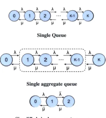
In this paper, we use the same decomposition of aggregate states as in Osorio and Wang (2012). Figure 2-1 shows the state transition diagram, before and after aggregating the

state space. Each circle in the diagram represents a state, and each arrow represents possible transitions between the states with their rates. Arrivals in the figure are

determined by the arrival rate A > 0 , and departures by the service rate p > 0

p p p p p

Single Queue

Single aggregate queue

A 2

p p

Simplified single aggregate queue

Figure 2-1: Aggregating the state space of a single queue to three aggregate states (Osorio and Wang, 2012)

Initially, we have M= K + 1 states, where K is the queue capacity. We aggregate to get M = 3 aggregate states. Our system now has only 3 aggregate states: aggregate state 0

representing an empty queue, aggregate state 2 representing a full queue, and aggregate state 1 representing a non-empty and non-full queue. For a network of queues, this means that the number of equations for the network is linear in the number of queues instead of exponential.

The third image in Figure 2-1 shows that the rates for leaving aggregate state 1 have changed. The other transition rates remain the same because aggregate state 0 and

disaggregate state 0 are equivalent. Additionally, aggregate state 2 and disaggregate state K are equivalent. The aggregate system is now fully described by a set of four rates

A, y, A and At. The first two are known and the last two (denoted aggregate arrival rate and

aggregate service rate respectively) can be defined from Equations (6), (7) (Osorio and Wang , 2012) and ( Schweitzer, 1984) as:

.(t) = A.PN=K-1(k

PA=1(t)

(8)

9T(t) it 0 = P P(N=1IA=1)

(9)

where PN=K-1, PN=1 are the probabilities that the queue is in disaggregate states K-1, I

2.2

Aggregate transient model for a single and a

network of tandem queues

In this section, we will apply the aggregation-disaggregation techniques from 2.1 to derive the model for calculating the transient queue-length distribution of a single M/M/1/K queue and the transient joint queue-length distribution for a network of M/M/I/K queues in tandem. We propose to calculate the joint transient distribution of a network of queues in tandem by decomposing the system into overlapping sub-networks of three queues. Below we present this formulation at three different network size levels: a single queue, a network of 3 queues in tandem, and a network of M queues in tandem.

2.2.1 Aggregate transient model for a single queue

For a single finite-capacity Markovian queue, the state space is given by fl =

to,

1,.., K}, where K 0 is the queue capacity. To derive the aggregate model for a

single queue-length distribution over time, we will use the same framework introduced in 2.1, where our system now has only 3 aggregate states. This results in a 3x3 aggregate

transition rate matrix, QA.

The model is implemented in discrete time, and within each time interval, we assume aggregate transition rates to be constant. To present the model, we introduce the following notation:

queue arrival rate;

It queue service rate;

p queue traffic intensity; K queue capacity;

p0 initial disaggregate queue-length distribution of the queue;

pA(t) aggregate transient queue-length distribution at continuous time t

pk (t) disaggregate transient queue-length distribution at continuous time t within time interval k;

Qk

aggregate transition rate matrix during time interval k;

Ak approximated queue arrival rate during time interval k;

Itk approximated queue service rate during time interval k; p k approximated queue traffic intensity during time interval k;

Ak aggregate arrival rate during time interval k;

k aggregate service rate during time interval k;

Pn probability of being in disaggregate state n at stationarity;

5 time step length;

T duration of entire time horizon;

t continuous time within the [0, 6] interval.

For a queue with arrival rate A, service rate p, capacity K and initial disaggregate queue-length distribution p0, the traffic intensity p is defined as the ratio of the arrival rate to

service rate p = -. The discrete form of the aggregate queue-length distribution over time

i

is defined as:

pA(t) = pj-1(6)e A, Vt E [0, 5], pA() =P

(IOa)

-A A 0

Qk _ k _ gk A k

0 it -P

(10b)

where the initial aggregate queue-length distribution and initial service and arrival rates are defined as:

PN=0 0 0

p0= 1-P=0-PK= 1 _ N=1

0 PA=1 PA=1

(10c)

To calculate the aggregate transition rates Xk, gk, we refer to equations (8) and (9). In

discrete time, we get:

k-1 t i A NK- _0K1) k -1A=1) (0 PA- (0) P(Nk-1=)J PA=16 (1 la) k-1 -k PN=1 ) k-1 ~ k-1 1 (N=1|A=l) (11 b) Equations (I la) and (1 b) require calculations of the disaggregate queue-length

distributions (i.e., p=1 (S), and pN-K _₁(6)). Since these are not available, we apply the

closed form expression of the queue-length distribution from Morse's exact method

(1958, p.65-67) to approximate the disaggregate distributions. The transient queue-length

distribution as derived by Morse (1958) in continuous time is given by:

PN=n(T) = Zr=PN=m d =n()

(12a - 1)

In discrete time at time interval k, the transient queue-length distribution is defined as:

pk=(t) = _{o pk-(S) dmk (t), Vt E [0, S],}

(12a - 2)

where po=m is the initial probability of being in disaggregate state m, p k1(0) is the

probability of being in disaggregate state m from the previous time step. In continuous time, dmN=(T) is defined as:

dm=n(T) =Pn

1 ) K

2p " 1 sm s(m +1) snw

+- sin -psin sinm

+ K+1 1xS K+ 1 K+1 I[ _fK+1

S=1

s(n+1)7 y

-Osin _K+1

(1 2b- 1) and in discrete time during time interval k with continuous time t, d 'd (t) is defined as:

dNi(t) = P

-6 m K

2p2

1

sm s(m + 1)7i snw

+ -sin - l- sin sin

K+I1 x K K+ 1 K+ 1 K+ 1 S=1 s(n +1)T - sinK +1 (12b-2) + P - 2 Aiicos (Ks+K1 (1 2c) where, P, = ( p)pn is the stationary distribution of an M/M/1/K queue, and n E

i-PK+1

[0,1,...., K]. Both n and k + 1 are exponents in the stationary distribution equation.

To approximate the disaggregate probabilities, pNj (6), and P-i(6), we solve a nonlinear system of equations for pk-1, Ak-1. The nonlinear system consists of two equations: The first states that pN=0(6) and pA-(6) are equal, and the second states that pN-K(6) and pA-2(6) are equal. We end up solving two nonlinear equations for two unknowns. The nonlinear system is defined below in Equations (13) and (14) and in more details in Equations (15) and (16).

pk-i(1) -pIk ()

-(

SPN~=m~(8)

k-2

dN=O'()

mkl,)=0

=0 m=O/

SpN~m(8)

d~7~() = 0 M=O

We plug Equation (12) into (13) and (14) and get

k-1i6 PA=o() - pm(5) PO S2(pk-1) K k-1 K +1 =I Ak-1 + k-1

-

2 Ak-lpk-io _(KsC

)

- sn (m + 1)7r in s -_(Ak-1 it-1_2a-p- o~ g K + 1 K + I =0, (15) (13) (14)

[sin

m

-~~ p- 2() m=0 (PK -(K-m) K k-1 + 2(+k1)2 -) _{- sS} K + A4k1+ pk1 -2V k-1k Coss) k s(m+ n i1) ] K + 1 1~i -(kl~t- _{__} Sin +

-

-2Ak-1pk-1Cos(TSi snK + 1 1 =0, (16)

where Ak-I k-1, are the queue arrival rate and service rate during time interval k - 1

k- k-1

that we want to solve for, and p - where k - 1 represents the time interval

index.

Once we solve for Ak-1 and pk-1, we plug them into the discrete form of Equation (12) with the initial disaggregate distribution p- 2 _{(6) to get the disaggregate probabilities} pN= 1 (6), and P=K_ 1 (6). The disaggregate probabilities will then be plugged into Equations (1 la) and (1 b) to calculate the disaggregate transition rates tk, fk.

The full algorithm for solving the transient distribution of a single queue can be described in the following steps:

Input:

Arrival rate to the queue: A Service rate of the queue: y Queue capacity: K

Initial disaggregate queue-length distribution of the queue: pN Duration of entire time horizon;T

Output :

T

Assuming that - is an integer, the output is an approximation of the aggregate queue-length distribution of a queue at time T (in discrete time at time interval

T

k= ): p (t), where t can be any value between [0,

S].

Algorithm:

6 can be initiated as any small number.

T

For k = 0,1,2,

If k = 0

1) Calculate the initial aggregate distribution (po) from the initial

disaggregate distribution (p') using the following equation:

p3=

[

0N=0PNO

1- Pn=0 - PN=KI'

0

PN=K

2) Calculate the initial aggregate transition rates 1, pal:

0 S PN=K-1 0 PA= 1 0 1 N=1 PA=1 Else

1) The aggregate queue-length distribution for time step k of continuous time t is defined as:

where pk(O) = pk-1 (S), Qk = [fk -0 A (k + It ,jk)

2) Solve the following nonlinear system of equations to obtain AkIk,

where dn Ik (6) is given by Equation (1 2b-2):

PA=o(6)

-PA=2(6)

-Z

k- mk (6) 0

PN=M(S5) d = 0

m=O

3) Plug Ak, yk into Equation (12) to get the disaggregate probabilities of

being in disaggregate states 1, K - 1:

k PN =K-10() K =

Ip-M(6)dN=kKl(

1 m=O K p=1() = Nph(6) d 1(S). m=O

4) Calculate Xk+1 gk+1 for the next time step from the following

equations: SPN=K-1(() pA₁() -k+1 __ =1 pA1()* End End

2.2.2

Aggregate transient model for a three-queue

tandem network

In this section, we consider three M/M/l/K queues in tandem. For this type of network, we want to approximate the aggregate joint queue-length distribution PA (t) which is defined as the probability that the first, second and third queue, are in aggregate states

i], respectively at continuous time t E [0, 5] within time interval k. The aggregate state

space is defined as the triplets with 27 unique states where (i,j, 1) E tO,1,2}3. Therefore, the dimension of the transition rate matrix is independent of the individual queue

capacities and is always 27x27.

We introduce the following notation:

N disaggregate state of queue i;

Ai aggregate state of queue i;

yi external arrival rate to queue i;

Pi service rate of queue i;

K capacity of queue i;

K capacity of the queue corresponding to blocking scenarioj;

approximated queue arrival rate for blocking scenario

j

during time interval k;

k approximated queue service rate for blocking scenarioj during time interval k;

p approximated queue traffic intensity for blocking scenario j

p1

during time interval k;

P=(i,j,1>(t) aggregate joint queue-length distribution at continuous time

t within time interval k;

P=ijI>(t) disaggregate joint queue-length distribution at continuous

P(Ai=a)(t) the marginal probability that queue i is in aggregate state a

at continuous time t within time interval k;

p(Ni=n)(t) the marginal probability that queue i is in disaggregate state

n at continuous time t within time interval k;

0initial disaggregate queue-length distribution for queue i;

p~i initial aggregate queue-length distribution for queue i;

P initial aggregatej queue-length distribution ;

P initial aggregate joint queue-length distribution;

P0(~j1 _{initial disaggregate joint queue-length distribution;}

QkAJ

aggregate joint transition rate matrix (AJ is a shorthand for aggregate joint) within time interval k;

kj empty aggregate transition rate probability for blocking

scenario j during time interval k;

fk full aggregate transition rate probability for blocking

scenarioj during time interval k; time step length;

T duration of entire time horizon;

t continuous time within the [0, 6] interval.

Each of the three queues in the network has an external arrival rate yi, service rate /i, queue capacity K and initial disaggregate queue-length distribution po,, where i E

{1,2,3}.

We calculate the initial disaggregate joint distribution pN=(i,,j1) by assuming a product-form joint queue-length distribution, i.e., the initial joint can be decomposed as a product of its marginals. Unfortunately, finite-capacity queueing systems, in general, do not have a product-form joint queue-length distribution. The reason for that is because finite-capacity queueing system give rise to blocking which might cause intricate

dependency between queues, where service and arrival rates of queues might increase of decrease depending on any blocking that might occur in the system.

When a queue is causing blocking on upstream queues, the service rates of upstream queues might get decreased because of the blocking. Additionally, when the queue causing the blocking has a service completion, service rates of some blocked upstream queues might increase. Hence, calculating the joint is a challenge in that blocking should be captured in all its scenarios and accounting for these dependencies between queues is necessary.

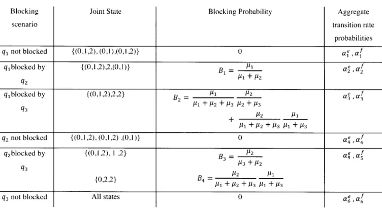
In a three-queue tandem network, where q, is the most upstream, q, can be either be not blocked or blocked by either q2 or q3, and q2 can either be not blocked or blocked by q₃,

and q3 is always not blocked. This gives us a total of 6 blocking scenarios. The

probability of a job being blocked for each of these scenarios has been approximated in Osorio and Wang (2012). Table 2-1 shows all these scenarios with an approximation of their probabilities of occurrence.

Blocking scenario

Joint State Blocking Probability Aggregate

transition rate probabilities q, not blocked {(0,1,2), (0,1),(0,1,2)} 0 ae f q1blocked by {(0,1,2),2,(0,1)} B1 = Yi aeaf /1 + P2 q2 q1blocked by {(0,1,2),2,2} B2 = /1 P2 ae , af S I1 + 112 + P3 /2 + P3 + P2 i P1+P2+p3 Y1+M3 q2 not blocked {(0,1,2),(0,1,2) ,(0,l)} 0 _{a4 , a4} q2blocked by {(0,1,2), l ,2} B3 = P2 aeaf B P3 + /2 q3 P2 P1 {0,2,2} B4 =

q₃not blocked All states 0

Table 2-1: All blocking scenarios with joint states, blocking probabilities, and aggregate transition rate probabilities

To calculate the transient joint queue-length distribution, we refer to Equation (10) from the single queue model and modify it to apply for the 3-queue joint model. The joint model is also implemented in discrete time, and within each time interval, we assume aggregate transition rates for all blocking scenarios to be constant. The main equations for the joint transient models is presented below in Equations (17) and (18):

pA=(i - pAj,)()e kl)-1) t J, Vt E [0, 6], pA (0) = p (5),

(17)

where

Q

= f(y, i, ak, B) is a 27x27 sparse matrix with nonzero elements given in appendix A. The parameters for the matrix are: y = [yi, Y2, Y31, P = [/1, P2,1 3],

[₁BBB ak = yek fk ek f k ek f k ek f k ek f k ek

B= [B1, B2,B3,B4],a - [a, a, , a2 a ,a3 , a3 , a4 la ₄ , as, a , a6

af ]. The initial aggregate joint queue-length distribution PA_(,j,]), is calculated

assuming independent initial marginal aggregate queue-length distributions of the three queues. To calculate it, we perform a cross product of the three initial aggregate queue-length distributions, where p 0 p 0

PA1=,I PA2=A 3=1*

We define the aggregate transition rate probabilities as follows:

k-1

ek = k-1 P(N1= 1|A2 *2)(5)

1 P((N1=1|A2*2)J(A 1=1I A2*2))(S) k-1

P(A1=1|A2*2)(6

k-1

fk k-1 P(N=Kl-1 A2*2)(S)

a1 P((N₁=K₁-iIA₂*2)1(A ₁=1|A ₂*2))() _k-1

P(Al=l|A2* 2) 0

k-1

ek k-1 P(N=iA2=2,A3*2)

a2 P((N₁=lIA₂=2,A₃*2)|(A _{1 =1lA 2}=2,A3*2))(.Y) k-i

P(A1=1| A₂=2,A₃*2)(S)

k-1

fk k-1 P(N=K1-1IA 2A2=2,A 3*2)(0)

2 P((N1=K-1I A2=2,A3*2)| (A=iI A2=2,A3*2)) k-1

P(A1=1|A2=2 ,A3*2)( 6

)

k-1

e k k-1 P(N1=1 IA2=2 ,A3=2)

3 P((N1=1| A2=2,A3=2)|(A1=1i A2=2,A3=2))((5) k-1

k k-1

k_ P(Nl=Kl-i |A₂=2 ,A3=2)()

3 P((N1=Ki-| A2=2 ,A3=2)I(A1=1 A2=2 ,A3=2)) k-1

P(A1=1|A2=2 ,A3=2) '

k-1

ek k-1 P(N2=iIA32)'.J

4 P((N2=1|A3*2)I(A2=1IA3*2))k = k-1

P(A2=1IA3*2)

k-1

f k k-i P(N2=K2-1 |A3*2)'() 4 P((N2=K2-1IA 3*2)1(A 2=lIA3*2)k = k-1

P(A2=1A3*2)()

k-1

ek _ k-1 P(N2=1|A3=2)(

7

)

5 ((N2=1IA3=2) I(A2=1iA3=2)) k-1

P(A2=1|A3=2) k k-1 ff k-1 P(N2=K2-1|A3=2) 5 ((N2=K2-1|A3=2) I(A2=1|A3=2))(5 k-1 P(A2=1|A3=2) k-1 ek __ k-1 _P(N 3= 1) (6) 6 P(N3=1|A3=1)(6 k-1 P(A3 =1)(6 k-1 afk = k-1 P(N3 =K3 -1) 6s -(N3=K3-1 IA3=1)(5 k-1 P(A3 =1)() (18)

For each of the 6 blocking scenarios in Table 2-1, at time step k, we define 2 aggregate

f k

transition rate probabilities, the full aggregate transition rate probability, denoted a, and the empty aggregate transition rate probability, denoted afk .a( represents the ratio of the probability of being in disaggregate state I given blocking scenario j to the

probability of being in aggregate state 1 given blocking scenarioj at time interval k-1. While af represents the ratio of the probability of being in disaggregate state Kj -1 given blocking scenario j to the probability of being in aggregate state 1 given blocking

scenarioj at time interval k-1.

Calculating the full and empty aggregate transition rate probabilities for all the blocking scenarios, defined in Equation (18), is somewhat of a challenge given that the

disaggregate probabilities in the numerators are unknown. To approximate the

is by assuming the disaggregate probabilities of the blocking scenarios follow the functional form given by Morse (1958) in Equation (12). We solve 6 different nonlinear systems for all blocking scenarios. We solve the nonlinear systems in Equations (19) through (24) to obtain six different pairs of A -' and p4-, wherej represents the blocking scenario index.

To approximate the disaggregate probabilities for blocking scenario 1: pk-=1A 2*2) P(N1=Ki-1|A2# 2)(6), during time interval k - 1, we solve the following nonlinear system

for Ak-' and pk- 1:

~k-1( 6 P(A=(A2*2) -PA1=2|A2*22 ) -K, k-2 P(Nl=mA 2*2) m=O K1 I 0 k-2 P(Ni=MIA2#2) (6) d mik-li(5)) 0, (6) d 0.k-N=j0

To approximate the disaggregate probabilities for blocking scenario 2:

P(N=1 A2=2,A3*2) P(N1=K1-1 |A2=2,A3*2)(

6

) during time interval k - 1, we solve the

following nonlinear system for A4-1 and p -1:

k-i P(A1=O A2=2,A3*2)( 6 ) -k-1 P(A1=2 IA2 2,A3*2)( 65) -K, k-2 P(Nj=mA2=2,A3*2) m=O P&Vil=mIA2=2,A3*2) (65) d m=0, N=Ok~ (6)) 0 (6) d 4) =~- 0. (20) To approximate the disaggregate probabilities for blocking scenario 3:

k-1= =A (N₁=K₁-1 2=2,A3=2((A6) during time interval k - 1, _{we solve the} P(N=in A2 nAie 2)ar), sefrKl- i And pA -:

following nonlinear system for 3 1 and .u 3i:

k-1 P(A1=O A2=2,A3=2)( 6) -k-i P(A1=2 1A2=2,A3=2)(6) -P(N1=m|A2=2,A3=2) K1 m P0(Nj=m|A₂=2,A3*2)

(m=O

(6) d m~7 )) 2 (6)(6 0 (21) To approximate the disaggregate probabilities for blocking scenario 4: p(N=|A3*2) ()

k--i

PfN2=K2-1|A32)(6) during time interval k - 1, we solve the following nonlinear system

for Ak-1 and plk-1:

K2 m 0(N2=M|JA32) k-P(A2=o IA3 *2)(6)-k-1 P(A2=2 IA3

*

2

)G(')-k-2 P(N₂=rn IA3*2)()

d

Jik-7(6)) 0, dKI(6) 0, k-1

To approximate the disaggregate probabilities for blocking scenario 5: p(N₂ =1 A3 =2)

P(N2=K2-1 IA3=2)(6) during time interval k - 1, we solve the following nonlinear system

for .- and p i-:

k-1 P(A2=0 IA3=2)( 6) -k-1 P(A₂=2 IA3=2)(6) -K2 m (N2=m IA3=2) (6) Mn= 0 k-2 |=K P(N2=M IA3=2)(5) dN = K,(5) (23)

To approximate the disaggregate probability for blocking scenario 6: pk-i 1(6),

PfN=K-) 3 (6), during time interval k - 1, we solve the following nonlinear system for

6L-1 and 6 -1:

K3 p(-3=)(6) - PNI=m)(6) dNl=- (6)) \m=0 K3 pk-1(s) - _{P$2-m) (6) d mk-1()) 0.} (24) For Equations (19) through (24), we calculate d ,k-1'(6), d iy-'(6) from equation (12b-2). Once A -' and y -' forj E{1,2,3,4,5,6} are obtained from the nonlinear solver, we plug them into the discrete form of Equation (12) to get the disaggregate probabilities needed. These steps are described in more details in the algorithm description below.

The full algorithm for solving the transient joint distribution of a three-queue network can be described in the following steps:

Input:

External arrival rates to each of the three queues : y = [yi, Y2, Y3].

Service rate for each of the three queues: p = [i 1, P2,

P31-Queue capacity for each of the three queues K = [K1, K2, KJ.

Initial disaggregate distribution for each of the three queues: po,, ps2, PN3

-Duration of entire time horizon: T.

Output :

T.

Assuming that is an integer, the output is an approximation of the aggregate queue-length distribution of a queue at time T (in discrete time at time interval ):

T

P 1(t,) where t can be any value between [0, 8]..

Algorithm:

( can be initiated as any small number.

If k =0

1) Calculate the initial aggregate distribution (p%,) from the initial disaggregate distribution (pt,) for iE{1,2,3} using the following equation: 0 PNi=O pi= -= Pi=K] 0 . PNi=K

2) Calculate the initial joint queue-length distribution from the following equation:

0 0 0 0

PA=(i,j,l) = PA1=i PA2=jPA3=1

3) Calculate the initial aggregate transition rates for each of the blocking

scenarios a, aP for i e {1,2,3,4,5,6} from the initial joint p0

sca rio anta a gtA=(ij)

and the initial disaggregate distributions po,, po2 0~3

0 el P(N1=11A2*2) a1 0 P(A_{1 =1IA2} *2) 0 el _ P(N=1| A2=2,A3*2) a2 _{0 '} P(A1=11 A2=2,A3*2) 0 a P(N1=1|A2=2,A3=2) 3 0 P(A₁=1|A₂=2 ,A3=2) 0 el P(N2=1IA3#2) a_{4 0} P(A2=1IA3*2) 0 e1 P(N2=1|A3=2) a_{5 k-1} P(A2=1IA3=2) 0 el P(N3=1) a6 - ₀ P(A3 =1) fl 1 fl 2 3 fa 4 fa 5 fa 6 0 P(N₁=Kl- 1JA ₂*2) 0 P(A₁=1|A2*2) 0 P(N₁=Kl-1| A₂A₂=2,A₃*2) 0 P(A₁=11A₂=2 ,A₃*2) 0 P(N₁=K₁-1| A2=2,A3=2) 0 P(A1=1|A2=2 ,A3=2) 0 P(N2=K2-1 JA3*2) k-1 P(A2=1| A3#2) 0 P(N₂=K2-1 |A3=2) 0 P(A2=1IA3=2) 0 P(N₃=K₃-1) 0 P(A₃₌₁₎ Else

1) The aggregate joint queue-length distribution for time step k of

continuous time t is defined as:

PA=(i,],) ( = P!;(bJ,)(6)et Q , Vt E [0, 6] ,

where Qk; = f(y, k , B) is a 27x27 sparse matrix with nonzero

elements described in appendix A. The parameters for the matrix are:

Y = [1, Y2, Y], = [11, Y2, A3] given initially as input ,

B = [B1, B2, B3, B4] given in Table 2-1, and

a k= a ek afk aek , fk ,aek , fk ,aek Y fk .aek

L1 1'2 a2 ,a3 a3 ,a 4 a 4,a 5 af kaek

af k

a5 6 a6 j

approximated in the previous time step.

2) Solve six nonlinear system of equations for the six blocking scenarios to obtain A, p where

j

is the blocking scenario index:

Nonlinear system 1: Solve to obtain I, 14 K, M=0

)=0

K₁ k-1 P(Ni=mIA2* 2)() m=O

Nonlinear system 2: Solve to obtain 29, 2i

k P(A₁=O |A₂=2,A3*2)( 6 ) -k P(A1=2 JA2=2,A3*2)() -K,

j

P (N1=m|A2=2,A3*2)(5) d ( )= K,

(

= 1 =K M= 0

Nonlinear system 3: Solve to obtain , p

d=K )

P(A1=0|A2*2)(6 P(N1=m|A2*2)(5 dN015

P(A₁=O |A₂=2,A =2)(S) -k P(A1=2 IA2=2,A3=2)(6) -K1 k-1 m P(N 1=m|A2=2,A =2)(J m=| YP(N=mA2=2,A3*2) (6)

Nonlinear system 4: Solve to obtain 4, y4

K2 m 0(N2=M|JA342)( k P(A2=0 IA3 2) k P(A2-=2JA3 #2)(S N=O(6) 0 K2 m 0(N2 =M A3*2) (6) K

Nonlinear system 5: Solve to obtain A5, p

k P(A2=O|A =2)( ) k P(A2=2IA3=2)G5') K2 M(0 K2 M=0

Nonlinear system 6: Solve to obtain A6, 6

K 3 p(A, =0) (6) - p(N3 =M) (5 M=0 K( P(A3=2)(m ) d (m( ) N =M()5) K )

3) Plug each pair A, p< and the disaggregate distribution for each

blocking scenario from time step k - 1 as the initial distribution into

the discrete form of Equation (12) to get the disaggregate probabilities

of being in disaggregate states 1, K - 1.

N=

K(6) 0

0 P(N2=m A3=2) (8) d20 (S)

Plug Li, p1 and the disaggregate distribution for this blocking scenario from time step k - 1 as the initial distribution, into Equation (12) to

get: K₁ P(N=1A 2*2)() = N=m|A2*2) m=O K₁ k )1= K

P(N1=,c1-11A 2*2) (6) = Y.P(Nj1 =mIA2*2)(6d= _ (6).

M=O

Plug

4,

p into equation (12) to get

k P(N1=1 IA2=2,A 3t2)( 8 ) k P(N1=K1-1 IA2=2A#)8 K1 m P0(Nj=m|A2=2,A3*2)(S) d N=1 m=O K1 (Ni=mIA2=2,A3*2)( 6) dNKl-l m= 0

Plug Xi 3 into equation (12) to get

k P(N₁=11A2=2,A3=2) () k P(,v₁=K₁-11A2=2,A3=2) (6) K₁ = P(Ni=m|A₂=2,A3=2)(6)dN=1(1)1 m=0 K1 S0 (N1=m|A₂=2,A=2)()dN=Kl_1- ). m=0

Plug i 4, into equation (12) to get

K₂

P(N2 = l|A3:2)(5 = I = P(N2=m|A3*2) ()Nl6)

K₂

(N2=K2-|A32)( = P(N2=mIA3*2) ()dN=K2- (6)

m=0 plug

Ak'

Il into equation (12) to get