Approximate models for stochastic load combination.

-1-APPROXIMATE MODELS FOR

STOCHASTIC LOAD COMBINATION

by

CHARLES BENJAMIN WAUGH

B.S.E., The University of Michigan (1975)

Submitted in partial fulfillment

of the requirements for the degree of

Master of Science in Civil Engineering

at the

Massachusetts Institute of Technology

January 1977

Signature of Author .

Department of Civil Engineer ig,' January 21, 1977

/

Certified by

...

.

...

.

.

.

.

.

.

Certfie/by

...

('/'"1

"-'"

''-'

''

Thesis

Supervisor

Accepted by . . . ..

Chairman, De ir mental Committee on Graduate Students of the Department of Civil Engineering

Archives

MAf 3

1977

ABSTRACT

APPROXIMATE MODELS FOR STOCHASTIC LOAD COMBINATION

by

CHARLES BENJAMIN WAUGH

Submitted to the Department of Civil Engineering on January 21, 1977, in partial fulfillment of the requirements for the degree of Master of Science in Civil Engineering.

This work deals with load combinations both from theoretical and practical viewpoints.

Starting first with theoretical considerations, load combinations are treated as mean outcrossing rate problems. A modified square wave (jump discontinuous) process is considered, and the expression for the outcrossing rate from a two dimensional region derived. This result is compared to results relating to multidimensional Gaussian processes.

Next, a series of case studies is carried out. These studies deal with reinforced concrete columns subjected to both time varying, random lateral and gravity loads. It is demonstrated that for cases of prac-tical interest, interaction diagrams may be replaced with linear bound-aries for purposes of reliability analyses.

It is also shown that by considering such linear boundaries, an outcrossing rate problem is reduced to an upcrossing rate problem, which

is simpler from both conceptual and computational viewpoints. Further simplifications relating to upcrossing rate problems are also presented.

Engineering practice is considered in terms of building design codes. Present codes are discussed, and then theoretical objectives of modern probabilistic codes are outlined. Finally, some recent draft proposals are considered. Using the methodology developed earlier, these are checked

for risk consistency. While no improvements on these formats are offered, it is concluded that such codified approaches appear to meet presently stated objectives.

Thesis Supervisor: C. Allin Cornell

Professor of Civil Engineering Title:

-3-ACKNOWLEDGEMENTS

Sincere thanks to the faculty at M.I.T., especially to Professor

C. Allin Cornell, without whose help and direction this work would not

have been possible.

Thanks also to the National Science Foundation, who sponsored the

author as a N.S.F. Fellow, and also for their sponsorship of this work

TABLE OF CONTENTS Page Title Page Abstract Acknowledgements Table of Contents List of Figures List of Tables Introduction 1.1 Motivation 1.2 Formal Definitions

1.3 Review of Other Work

1.4 Issues of Modeling

1.5 Purpose and Scope of Research

Load Combinations as Mean Outcrossing Rate Problems

2.1 Outcrossing Rate Results for Modified Square Wave Processes

2.2 Outcrossing Rate Results for Gaussian Processes

2.3 Case Studies: Reinforced Concrete Columns

2.3.1 Parameter Selection 2.3.2 Computational Procedures 2.3.3 Study 1 2.3.4 Study 2 1 2 3 4 6 8 Chapter 1 Chapter 2 9 10 10 23 35 37 42 47 48 52 53 61

2.3.5 Study 3

2.3.6 Conclusions drawn from Case Studies

2.4 Linearizations in Load Effect Space

Chapter 3

Chapter 4

Chapter 5

References

Scalar Load Combinations Problems

3.1 Upcrossing Rates for Scalar Sums of Processes

3.2 A Markovian Approach

3.3 Further Simplifications

3.3.1 Results for High Failure Thresholds

3.3.2 Transience 3.4 Computational Procedures Engi 4.1 4.2 4.3

neering Practice for Load Combinations

Past and Present Practice

Theoretical Objectives in Codified Design

Recent European Developments

4.3.1 C.E.B. Drafts

4.3.2 N.K.B. Draft

4.3.3 E.C.E. Draft

4.3.4 Reliability Consistency of the European Formats

Conclusions and Recommendations

Appendix: Computer Programs

-5-67 74

80

-6-FIGURES

Page

1.1 The Borges--Castenheta model. 12

1.2 Structural interaction in the work of Borges and Castenheta. 13

1.3 Effect of adding a probability mass at the origin of a 16 distribution function.

1.4 Hypothetical realizations of modified square wave processes. 17

1.5 Three equivalent load combination formulations. 19

1.6 Event representation of a thunderstorm. 26

1.7 Event representation of a severe thunderstorm. 26

1.8 Effect of excessive variability in the secondary process. 29

1.9 The effect of filtering. 30

1.10 Interpretation of influence coefficients. 33

2.1 Hypothetical realization of a two dimensional square 38 wave process.

2.2 Important points on the failure boundary. 38

2.3 Integrations involved in the two dimensional modified 40 square wave process.

2.4 Outcrossing of a two-dimensional Gaussian process. 45

2.5 Details of the segment B.. 45

2.6 Reinforced concrete column parameters. 50

2.7 Interaction diagram in load effect space, study 1. 55

2.8 Interaction diagram in load space, study 1. 55

2.9 Reduced space diagram, cases 1A and 1B. 56

2.10 Reduced space diagram, case 1C. 56

2.11 Continuous and jump process results, study 1. 57

-7-2.13 Interaction diagram in load effect space, study 2. 62

2.14 Reduced space diagram, study 2. 63

2.15 Continuous and jump process results, study 2. 64

2.16 Linearizations of the jump process, study 2. 65

2.17 Interaction diagram in load effect space, study 3. 69

2.18 Reduced space diagram, study 3, cases A - D. 69

2.19 Reduced space diagram, case 3E. 70

2.20 Reduced space diagram and amended linearization, case 3E. 70

2.21 Continuous and jump process results, study 3. 71

2.22 Linearizations of the jump process, study 3. 72

2.23 Approximations of circular boundaries by a line. 77

2.24 Approximation of an elliptical boundary by a line. 78

2.25 Transformation of the failure region into an open domain. 79

2.26 Veneziano's searching scheme. 82

2.27 Linearizations in load effect space. 83

2.28 Linearization example in load effect space. 87

3.1 Relationship between square wave processes and Markov 95 states 0, 1, 2, and 1*2.

4.1 Case A, normal distributions. 123

4.2 Case A, gamma distributions. 123

4.3 Case B, normal distributions. 124

4.4 Case B, gamma distributions. 124

4.5 Case C, normal distributions. 125

TABLES

Page

1.1 Intervals assumed by Borges and Castenheta. 13

2.1 Parameter Values and Results for Study 1. 60

2.2 Parameter Values and Results for Study 2. 66

2.3 Parameter Values and Results for Study 3. 73

4.1 (After the C.E.B.) Recommended ys values. 111

4.2 (After the N.K.B.) Recommended ys values. 116

CHAPTER 1

-9-INTRODUCTION

1.1 Motivation

Civil engineering structures are subjected to an environment comprised

of a host of different loads. Natural phenomena, such as wind, snow, or

temperature, and the actions of men, such as building occupancy loads must

all be considered. In the face of this, the engineer is charged with the

responsibility of designing structures that are both safe and economical.

Since these two aims are contrary, a balance must be struck.

Traditional-ly, this balance depended only upon the judgement of the engineer and those

he serves: architects, owners, and building authorities.

Recently, probabilistic methods have been advanced in a quest to aid

the design process. Engineers now generally accept the notion that both

loads and a structure's resistance to them are random in nature.

Further-more, rational methods to choose load and resistance safety factors have

been proposed. These typically assume knowledge of only the means and

variances of the random variables pertaining to any problem, and so are

known as second-moment methods. Important contributions have been made by

Cornell [13], Ditlevsen [15], Hasofer and Lind [25], Paloheimo and Hannus

[30], and Veneziano [39].

However, while these second-moment methods are capable of considering

multiple loads and resistances, in and of themselves they do not account

for a very significant aspect. All fail to explicitly treat the stochastic

(temporal) variability of loads. That is, loads are considered to be

re-search into structural safety. On the contrary, it is widely recognized.

Basic mathematical research is still underway, and furthermore, so are

in-vestigations of how to apply such results to practical needs. Both

consti-tute aspects of stochastic load combination.

1.2 Formal Definitions

Stochastic load combination problems are those for which the safety

or serviceability of structures depends upon multiple loads that vary

ran-domly in time.

In this work, stochastic load combination is to be distinguished from

either probabilistic or statistical load combination. Problems that

con-sider loads modeled simply as random variables (i.e., that do not

explicit-ly consider variation in time) we call probabilistic. Statistical load

combination deals with the application of data, either real or simulated,

to the task. Clearly then, probabilistic load combination is less general

a field of study than stochastic load combination. On the other hand, the

study of statistical load combination involves an entirely different

empha-sis and set of mathematical tools.

1.3 Review of Other Work

There is a paucity of modern work dealing with stochastic load

combin-ation. Therefore, this section will be able to examine the work in

moder-ate detail.

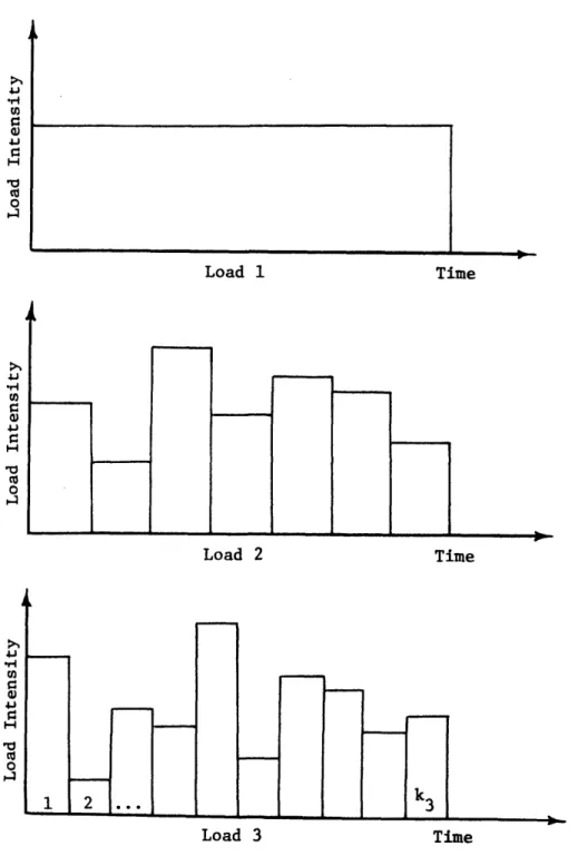
-11-model each load as a random sequence of values that are constant during

elementary intervals of fixed length. This is illustrated in figure 1.1.

Values of load intensity are assumed to be mutually independent, both

with-in a given load process or between processes. Table 1.1 with-indicates the

dur-ation of the elementary intervals for different types of loads considered,

as well as the total number of repetitions so obtained for a 50 year period.

Given the above assumptions, the probability of a n-dimensional load

vector S falling within the domain ds1, ds2,...dsn at least once during the

structural lifetime was found.

However, the result is difficult to apply, and so a simplified result

is also presented. It assumes the first load to be a dead load (i.e., k =

1 in the illustration, figure 1.1) and that there is only a small

probabi-lity that two other loads will occur in combination with it:

f(S)dslds

ds

k

fl(S1 )f

(s

)fk

(s

)dS

dS

ds

(.1)

3/k2

where the fi(-) and Fi(') are p.d.f.'s and c.d.f.'s relating to individual

load intensities within elementary intervals. The k's are the number of

repetitions, with k3 > k2 > kl, and:

k3/k

fkk (S3) = d[F3(s3) 2

3/k2

This is the expression actually used for the rest of the Borges-Castenheta

book.

Careful inspection reveals that the equation 1.1 is not a proper

Load 1 Time

Load 2 Time

Load 3 Time

Figure 1.1: The Borges--Castenheta model.

.rq w U) O .-I H 0 ed 0 r.l U) -I H C, la 0 '.4 4IJ -H-M 0 .-H 0 '.4

- -13-Table 1.1 (After Borges and Castenheta)

Intervals assumed by Borges and Castenheta

Duration of each elementary interval 50 years Number of independent repetitions in 50 years 1 Live load on buildings Wind 10 years* 2 years 1 hour Earthquakes 30 seconds

*Duration depends on the occupancy type.

S S s_{4 S} * s₃ 7 rrTT 5

L

Figure 1.2 (After Borges and Castenheta)

Structural Interaction in the work of Borges and Castenheta. Load Type Permanent 5 25 50 x 103 50 x 106 I 4

that the vector will fall into the region around (sl,' 2' s3) exactly one

time during the lifetime considered, and never in any other region. That

is, a distribution function must account for the probability of any single

(exclusive) outcome. However, it actually accounts for the probability

that the event occurs one or more times among many outcomes. Borges

as-serts that the two probabilities should approach each other if they are

suf-ficiently small. Therefore, equation 1.1 is offered as such an

approxima-tion. The assertion is reasonable, but evidence has not yet been offered

in its support or to bound its range of validity.

The transformation from loads to load effects is also considered.

Al-though non-linear structural behavior is discussed in general terms, most

of the study assumes a linear transformation from loads to effects. Figure

1.2 is an example of such a transformation, which can be expressed

concise-ly in matrix form:

q = [c]

where loads are denoted by s, their effects by q.

While it is shown in general terms how to use an expression such as

equation 1.1 to compute failure probabilities, computations are not carried

out. Instead, four examples combining loads on the structure were worked

out to the point of plotting lines of equal probability density resulting

from equation 1.1. Study of these examples may help to motivate an

intui-tive understanding of the nature of load combination problems. They do

not, however, lead directly and unambiguously to simple methods for the

se-lection of design loads or load factors.

Bosshard [9 ] generalized the elementary interval model of Borges and

-15-in the sense of summ-15-ing scalar values. These two po-15-ints will be discussed

in turn below.

The generalized model proposed by Bosshard consists of a Poisson

square wave process with a mixed distribution on load intensities. The

latter feature calls for the inclusion of a new parameter, p, which is the

probability that after any given Poisson renewal of the process, a zero

value of intensity is assumed. The effect of the inclusion of this new

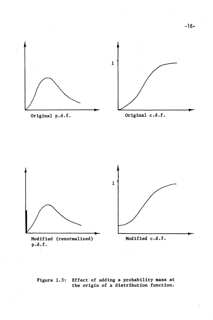
parameter is illustrated in figure 1.3. Successive renewals are again

as-sumed to be independent. Poisson square wave models had been used

previ-ously, such as in Peir's study [32], and with mixed distributions, such as

in McGuire [29], but those studies did not appreciate the significantly

greater modeling flexibility the introduction of p permitted. For

in-stance, if we set p = O, then the result is the familiar Poisson square

wave process discussed by Parzen [31]. On the other hand, let p have as

its compliment q = p - 1. Then, if the Poisson renewal rate is v, the

ar-rival rate for nonzero renewals is qv. Holding times between renewals are

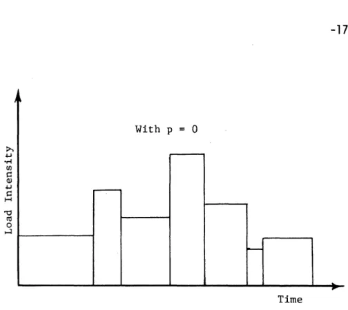
exponentially distributed with means of 1/v each. Hypothetical

realiza-tions of such a process are illustrated in figure 1.4.

Previous attempts (at M.I.T. and elsewhere) to represent infrequent

loads with random durations had focused on less convenient "three

para-meter" models, in which the load durations are arbitrarily distributed,

in-dependent random variables. These models were non-Poisson, and hence less

tractable. Examples are provided in the collection by Grigoriu [21].

In order to study the problem of summing the processes, Bosshard

adopted a discrete state Markov approach. Each process is allowed to take

1

Original p.d.f.

1

Original c.d.f.

Modified (renormalized) Modified c.d.f. p.d.f.

Figure 1.3: Effect of adding a probability mass at the origin of a distribution function.

With p = 0

With p close to 1

Figure 1.4: Hypothetical realizations of modified square wave processes.

-17-4-J ur H o 0 Time u₄₁ u as .H a -10

n

all possible combinations of these two sets. Bosshard showed how this

chain could be used to find the (discretized) extreme value distribution

for the sum of two processes over a given reference period. Using simple

two level discretizations on two processes, he studied then the coincidence

problem, or the probability that the two processes will combine, each

non-zero, during a reference period. Although his Fortran program would allow

studies utilizing the full power of his approach, such as extreme value

distributions for cases with more interesting distributions on the

indivi-dual processes, such studies were not carried out. In part, this is

be-cause the approach is computationally expensive (as some limited experience

with his program by researchers at M.I.T. has indicated).

Veneziano, Grigoriu, and Cornell have studied combinations of

indepen-dent smooth Gaussian processes [40]. Results are given for the mean rate

of outcrossing from a "safe" region in n dimensions. Simplifications are

found for spheres and polygonal regions. These results have an important

role in this work, and deserve to be presented in detail not appropriate to

this section. Instead, they are presented in section 2.2.

While the above three references represent recent work specifically

addressed to load combinations problems, there are earlier studies which

have laid the foundations for them. Gumbel wrote a treatise on asymptotic

extreme value distributions which is now considered to be a classic [23].

Rice did fundamental work dealing with mean-crossing rates for Gaussian

processes [34]. Ditlevsen [16], and Crandall and Mark [14] are other

ex-cellent references on extremes of Gaussian processes.

In summary, note the three approaches to problem formulation that have

19-T Time - -

Threshold

level

z

-S

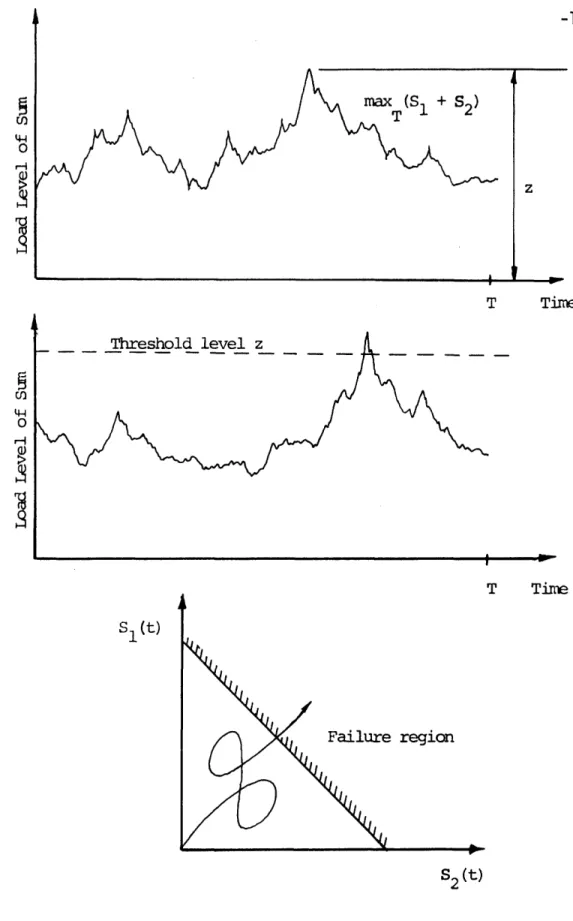
(t)

Figure 1.5: Three equivalent load canbination formulatiops. a 44 0 r--0 co H a, Is

upcrossing above a threshold level, and mean rates of outcrossing from a

safe region (e.g., in two dimensions). These are all illustrated in figure

1.5. Actually, these approaches are equivalent. First of all, the

proba-bility that the extreme value distribution of the combination is less than

a given level is exactly the same as the probability that there are no

up-crossings of this threshold:

P max (S + S2) = z

=

1

LT 1 2 j L threshold z, before time T J

Further, since the safe region in the last illustration is linear, the

problem is again of the form Sc = S1 + S2, and so is equivalent to an

up-crossing problem. This equivalence is discussed with more precision and

detail in section 2.4.

Other work bearing on load combinations has grown out of other

re-search topics in civil engineering reliability. Two examples are presented

here.

C. J. Turkstra has studied the decisions involved in structural design

[36]. In the course of his work, he considers probabilistic design formats,

including combinations of dead, occupancy, wind, and snow loads. The

an-nual maximum total load, or its scalar load effect, is sought. He proposes

that:

A reasonably simple expression for nominal maximum annual total loads ST is obtained if it is assumed that on the day when one q load reaches its annual maximum, other loads are chosen at random from the populations of their daily maximum loads....

Then, he proposes that the parameters of the total load on any of the

-21-E(S E(Sj + E(Si ) daily max (1.2a)

m ijai

Var(ST ) - Var(Sj max) + Var(Si daily max) (1.2b)

Or, as Turkstra wrote them:

E(ST) E(Sj max) + aiE(S_i max) (1.3a)

Var(STj)

T

jj

max

i

Vr(S

)

l3max)

where S_i max and Sj max refer to annual maxima of loads i and j, and a_i

and b_i are constants depending upon the location and use of the structure,

with a < 1. This is to say, he proposed that the parameters of the loads

related to daily maximum values be related to annual extreme value

infor-mation. In either set of equations, note also that individual loads are

to be "rotated", each in turn assuming the leading position where the

an-nual maximum is considered.

Clearly, the approach tends to be unconservative, in that it does not

account for possible maximum values resulting from combinations where none

of the loads is at an individual maximum. However, consider the effect of

another assumption. Denote by P(ST < z) the probability that the total

maximum effect is less than z, with load j at an annual maximum. Assume

that these probabilities are independent, even though it is generally not

true. Then, we may approximate the result relating to the maximum total

ST, regardless of the relative values of individual loads:

P(ST z) = P(ST ~ z) (1.4a)

The assumption of independence tends to be conservative. In situations

where a single load is dominant, the approximation should improve; this was

reported by McGuire [29]. A result complimentary to equation 1.4a simply

sums exceedance probabilities:

P(ST > z) = P(ST > ) (1.4b)

all i i

which as an approximation to 1.4a is conservative.

Turkstra's approach has the advantage that it is easily translated

into design rules for practical structural codes, each critical case being

represented by a deterministic load combination checking condition. In

fact, it is the basis for rules in both U.S. and European proposals, as

will be discussed in Chapter 4.

Hasofer considered the extreme value distribution resulting from the

superposition of a Poisson square wave with a Poisson event process, that

is, a process with no time duration. The research grew out of a study

dealing with floor live loads [24]. It is made more interesting by the

fact that it is an exact result. Further, it demonstrates how

mathematic-ally difficult an exact (versus approximate) result may become, since it

requires the solution of two integral equations; Hasofer did this

numeric-ally.

Of course, there are other studies which dealt with load combinations

or related topics. However, the goal here is not to provide a complete

and detailed review. Instead, the work that has been reviewed in detail

-23-1.4 Issues of Modeling

Load combinations has been a little explored field until recently. As

a result, basic issues concerning mathematical modeling of load combinations

remain. This section will address some of these issues, and then will

se-lect and define the features of a model to be used in the rest of this

thesis. The implications of the features selected will also be explored,

with particular regard to the limitations they impose.

Three basic model qualities are desirable:

1. The model must be useful for dealing with codified design.

2. The model must not demand any more information than can reasonably be

supplied.

3. The accuracy of any approximations in mathematical methods used must be

subj to verification.ect

To with codified design deal means of tat both the issnput and output of

the model must bear directly upon the desig p n rocesxample, if

loading codes define wind loading in terms of pressures, the model should

also deal in termplications pressures, not of sectral density curves that must be

further translated. On to the limitations the output must contain useful

in-formation for some safety checking scheme. So, for example, it is not

enough to know the probability that earthquake forcesir and snow loads will

act

concurrently

ust

bructure

usexactly

deauring

once

its lcodife.

Inforgn.a-tion

about intensities is anecessary. The distribumation than cane of lifetime

maximum moment in a par dticular member due to the superposition of the two

load processes would be an al ternative of g reater value.

The quality that the model must not demand too much information is

also deal in terms of pressures, not spectral density curves that must be

further translated.

On the other hand, the output must contain useful

in-formation for some safety checking sheme. So, for example, it is not

enough to know the probability that earthquake forces and snow loads will

act concurrently upon a structure exactly once during its life.

Informa-tion about intensities is also necessary. The distribuInforma-tion of the lifetime

maximum

moment in a particular

member due to the superposition of the two

load processes would be an alternative of greater value.

dictated by the limitations of practical situations. There is simply very

little data on the processes, natural or man-made, that contribute to

struc-tural loading. Estimates can be made, according to engineering judgement.

Such estimates contain valid information, and the model sets up a formal

framework for using it. However, a deeper discussion of this issue leads

into the realm of decision theory, such as Grigoriu dealt with [22].

Accuracy, in the context of this discussion, can only be defined in a

relative sense. We do not know the true state of nature. So, we cannot

state the true probability that the moment in a beam produced by two loads

in combination exceeds a given level at a given time. Yet, given some

as-sumptions, we may be able to get a closed form result, an "exact" result

for our purposes. Then, if a simpler approach is adopted for the purpose

of codification, it can be judged by the former standard.

Therefore, a premise advanced here is that simplicity is a helpful,

perhaps necessary model quality. Simplicity also has an advantage inasmuch

as it helps to clarify, rather than obscure what is actually occuring.

Long span bridge loading provides an example. Asplund used a very simple

model to study the reduction of lane loads with increasing bridge length

[ 4]. His model neglects consideration of the number or spacing of axles

on trucks, truck size distributions, vehicle headway, and other aspects

con-sidered in more recent research. However, his paper showed clearly why

lane loads should be reduced with increasing span length, and thus verified

an intuitive notion previously held by engineers.

In his work on model selection, Grigoriu also recognized the value of

model simplicity [22]. He studied the question in a more formal manner

-25-Taking all of the above into consideration, the following model

fea-tures are selected:

1. The model will consider the combination of only two load processes.

2. Each load will be modeled as a modified square wave, as proposed by

Bosshard.

3. The reliability information will be expressed in terms of mean crossing

rates.

Let us now detail the implications of these features.

First, combinations of three or more loads cannot be directly

con-sidered. This is because the sum of two processes, with either p O, is

no longer a Poisson renewal process, the only renewal process for which

superpositions are also renewal processes; see Karlin and Taylor [26].

However, combinations of lateral wind and floor live load, of interest for

many buildings, may still be considered.

Second, the use of the model as formulated by Bosshard poses the

ques-tion of how to model individual load processes as a series of distinct

events. This places a burden on researchers who are attempting to model

individual load processes. They must model loads in terms of p, v, and a

single distribution function relating to intensities. For example, imagine

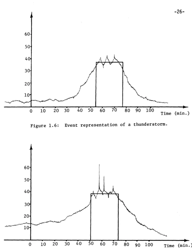
that figure 1.6 represents the measured wind speed before, during, and

after a thunderstorm. The bold lines indicate the way that the storm must

be modeled. Questions to answer include when does the storm begin, when

does it end, and what is its representative wind speed? Let us see how

such questions may be approached.

One might say that the storm begins when an upward trend in wind speed

601 50' 40 30. 20' 10' /

0 10 20 30 40o 50 60 70 80 _{90 100 Time (min.)}

Figure 1.6:

60'

50'

40,

Event representation of a thunderstorm.

- - I-. - - - .L .Lul1 LA /

Figure 1.7: Event representation of a severe thunderstorm.

I ...

~~~~

A A I",

-

'·_

_- -27-storm ends. For figure 1.6 we might judge that the -27-storm begins between

minutes 30 and 40, and ends somewhere after minute 100. However, the wind

speeds are still low at these points, not of interest to structural

engi-neers. Instead, let us focus attention on wind speeds above 35 miles per

hour. Then, say that the event representation of the storm begins when

sustained speeds of greater than 35 m.p.h. begin, and end when such speeds

are no longer sustained. By sustained, we may mean that the velocity must

remain above the reference level for all but short periods of time, say 20

seconds. Then, the representative velocity might well be taken as the

mean velocity during this period of event representation.

The problem then becomes the selection of the reference (threshold)

level of wind velocity. In the example illustrated by figure 1.6, 35 m.p.h.

would seem a good choice, because it is close to the chosen representative

velocity.

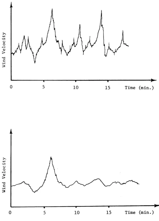
However, some problems may be more difficult. Figure 1.7 illustrates

what may happen during a severe thunderstorm, with short gusts of more than

50 or 60 m.p.h. Again, 35 m.p.h. was chosen as a reference level, and

again the representative value is not much greater. Yet, due to gusts

there is a much greater variability about the representative velocity. We

may attribute this variability to a secondary stochastic process; whereas

the primary stochastic process describes the arrival of storms with

repre-sentative velocities, the secondary process describes the gustiness about

this velocity. This secondary process may even be required to account for

the possibility of long waves, of perhaps 20 to 30 minute periods. The

to-tal static structural effect during any event is then due to the random but

secondary process. The proposal here implies that only the primary

compo-nent of the process will be properly represented in the analysis of

tempor-al combinations with other loads. The constant-in-time (i.e., the square

wave) assumption greatly facilitates this analysis.

It is important, for the purpose of the accuracy of this model, that

the secondary stochastic process contain relatively little variability

com-pared to the primary process. This condition reduces the probability that

(in the case of our example) the maximum lifetime wind velocity or its

structural effect occurs during an event other than the one with the

maxi-mum representative velocity, a situation illustrated in figure 1.8. It

also reduces the probability that the maximum effects due to the

combina-tion of wind with other loads occurs at a time other than that which the

model would suggest. Criteria for comparing variability in the primary and

secondary processes might take the form of keeping an acceptably low ratio

of the variances of the two processes. Unfortunately, formation of such

criteria goes beyond the scope of this work.

Structural interaction must also be considered. Figure 1.9

illus-trates a possible realization of the secondary stochastic process for

thun-derstorms, and the resulting bending moment in a particular member of a

structure subjected to the storm. Even if we do not consider the dynamic

characteristics of the building, there may be a filtering effect. Such

filtering may be due to one or more of many reasons.

Again using wind for example, filtering may be due to the fact that it

takes time for a gust to envelope a building; and by the time the gust is

beginning to have an effect, it is dying down. Such interaction requires

pro-ITOIyA puTM

-30-0 5 10 15 Time (min.)

5 10 15 Time (min.)

Figure 1.9: The effect of filtering.

4 U 0 ,1cr a) Ij_r4 .H c) U 0 a) ·I-Io w 10 0r .,. 0

-31-cedures involve only pseudo-static analysis. Therefore, it is left to code

committess and researchers modeling storms to select a transfer function

typical of the class of buildings being designed, to check and see that the

residual variability of the secondary process, left after filtering, is

acceptable.

There may be too much variability left after filtering. In such a

case, it may be an alternative to model storms as consisting of either

sus-tained winds or peaks. This is similar to the idea of using sussus-tained and

extraordinary load processes in floor live load modeling [32]. Yet, there

would be a significant difference. In the case of wind loading, the two

processes would be mutually exclusive, and so would not create a load

com-bination problem within the modeling of a single load type.

Consideration of structural interaction leads also to the topic of

variable space. When we speak of the space of variables, we are simply

re-ferring to the physical meanings of the quantities represented. Load space

variables deal directly with load phenomena, such as wind pressure, the

weight of furniture on a floor or snow on a roof, etc. On the other hand,

load effect variables refer to the results that loads subject a structure

to, such as bending moment or axial force. It is the behavior of the

structure itself in translating loads to effects that defines a mapping

be-tween the two spaces. We must decide which space we wish to work in.

There are advantages to working with either loads or effects.

Usual-ly, fewer effects are considered than loads. For instance, live floor

loads, wind and earthquake loads, and snow loads may be considered;

how-ever, at the same time, at most only axial and bending effects may be

such as ultimate moment capacity. However, loading codes deal in terms of

loads, not effects. Furthermore, it is usually assumed that loads act

in-dependently. In terms of modeling, this assumption becomes one of

stochas-tic independence. Yet, effects are usually not independent. For an

ele-mentary example, consider the case of a reinforced concrete column

sub-jected to both gravity and wind loading.

Let us assume linear elastic structural behavior, for simplicity.

Further, assume the fixed spatial loading pattern of uniform loads. Then,

adopting the same approach as Borges and Castenheta, relate the floor and

wind loading to the moment and axial effects, M and P, by a matrix:

M CWM CLM W

:WPCW

1C

(1.5)

P CWP c L

An interpretation of the coefficients of this matrix is illustrated in

figure 1.10.

Consider a point in time at which it is known that both wind and live

loads are acting at random levels. Assume knowledge only of means and

variances, and that the loads are not correlated. Then, the covariance

be-tween effects is found by simple linear operations:

2 2

Cov(M,P) = wCwp a + CLMCL (1.6)

which is generally nonzero.

The method adopted here is to invert the matrix [C], and translate the

description of the safe region into load space. Denote the inverse by [D].

-33-AW 0 L I \ N CWM = A Cos e H CWP = A_W Sin CLM= AL CLP = AL

Interpretation of influence coefficients. 11

I

I ,

{

L2

PLI

(1.7)

Lu dML dpL Pu

Proceeding point by point, we can define a new diagram in terms of the

loads themselves. Using this new diagram, safety analyses can be carried

out, in terms of the load processes only.

No matter what space of variables is selected, the failure surface may

be irregular and difficult to describe analytically. In such cases, it may

be desirable to replace the surface by simple approximations, such as

spherical or circular segments, planes or straight lines. Especially with

the latter approximations, considerable mathematical simplifications may be

achieved, as will be demonstrated in the next two chapters.

Finally, let us examine the usefulness of mean outcrossing rates as

reliability information. Structural failures are rare events. Due to this

fact, and also because we focus on high load and load effect levels, it may

be assumed that these rates pertain to Poisson processes. Then, the

proba-bility of the total load outcrossing the safe region (or exceeding a

thres-hold), denoted pf, is

pf = 1 - P(No outcrossing in [0, T]) = 1 - exp(-v+T) (1.8)

where v+ is the outcrossing rate. By taking the first term in the Taylor

series expansion for the exponential function, we obtain:

Pf < v+T (1.9)

which for small pf, is a good, while conservative approximation when taken

-35-1.5 Purpose and Scope of Research

As implied by the title of this thesis, its main goal is not only to

study models of load combinations, but also the effect of approximations

on them. Toward this end, each succeeding chapter will contain more

ap-proximations than the one before. At the same time, progress will be made

toward findings of practical value.

In Chapter 2, load combinations will be studied as mean outcrossing

rate problems. The outcrossing rate problem for the modified square wave

process will first be solved. Then, as an approximation, the continuous

process results of Veneziano, Grigoriu, and Cornell will be presented.

Comparisons made in the form of case studies will show that the continuous

process results often well approximate those of the modified square wave.

Additional insight is also gained by their use.

Also in Chapter 2, it will be shown how two dimensional failure

boun-daries may be linearly approximated. This offers the great advantage of

reducing the two dimensional outcrossing problem to a scalar (one

dimen-sional) uprcrossing rate problem. A method to perform these

lineariza-tions in load space is presented, and the resulting error and limitalineariza-tions

discussed in a series of case studies dealing with reinforced concrete

columns. A more direct method for performing such linearizations, in

terms of load effects, is also suggested.

Advantages gained from adopting a scalar boundary are exploited in

Chapter 3. The mean upcrossing rate for the sum of two modified square

wave processes is found. A Markovian approach similar to but distinct

in-sight. Even further simplifications, useful in certain special cases, are

also presented.

Code procedures for dealing with load combinations is the subject of

Chapter 4. Past and present development of practice is summarized.

More-over, the theoretical objectives modern code writing authorities hope to

achieve are presented, which links this chapter to the previous ones.

Lastly, it is shown how the stochastic model results of Chapter 3 can be

used to evaluate the degree to which simple codified formats are meeting

these objectives. A brief example of such a study is actually given.

Finally, Chapter 5 will offer general conclusions based upon the

en-tire body of this work. Recommendations for future research will also be

-37-CHAPTER 2

LOAD COMBINATIONS AS MEAN OUTCROSSING RATE PROBLEMS

2.1 Outcrossing Rate Results for Modified Square Wave Processes

The result for the mean outcrossing rate for the combination of two

modified square wave processes is found by a conceptually straightforward

argument. It is valid, however, only for processes that are independent

both in terms of temporal characteristics and in values of load

intensi-ties associated with renewals.

A hypothetical realization of a two dimensional combination of a

modified square wave process is shown in figure 2.1. This illustration

emphasizes the principle that the probability of simultaneous change is

negligible. Therefore, the problem can be split into two parts,

consist-ing of findconsist-ing the mean rates of outcrossconsist-ing associated with changes in

loads 1 and 2 separately. Let us focus on the mean rate of outcrossing

associated with changes in load 1 first. The result relating to load 2

is then similar.

Before proceeding, though, let us introduce some less precise but

shorter language. Though one must be mindful of their nature as expected

values, let us refer to rates of outcrossing, rather than mean rates.

Further, when referring to outcrossings associated with changes in a given

load, we shall simply allude to outcrossings "due" to that load. These

conventions will be used in the sections that follow.

Symbolically, denote the rate of outcrossings due to load 1 by vl+.

The rate vl+ is related to the rate vl by the probability that any

>4 x ta xC co₀₁ Ce 0 4 -o 03 'H cO 0 C, 4i 0 k4

4C)

-39-There is an There is a change

v+= v₁P

joutcrossing

J

Further, since the two load processes are independent, it is convenient to

condition upon the level of load 2. So, using this fact:

_V i pJ There is anlThere is a change in ds

1+ V 1 J outcrossingiload 1, and S2 = 2 2

To make the above result more explicit, we need to consider the forms

of the distributions relating to the intensities of loads 1 and 2. Let us

denote with a prime the modified and renormalized distributions obtained

from considering Fl(s1), F2(s2), P and P2

Fl'(Sl) = P1 + qlFl(sl) (2.1a)

F2'(s2) = P2 + q2F2(s2) (2.1b)

(Recall that the effect of including a probability mass p was illustrated

in figure 1.3.) It should be emphasized that these primes have no

rela-tion to the operarela-tion of differentiarela-tion.

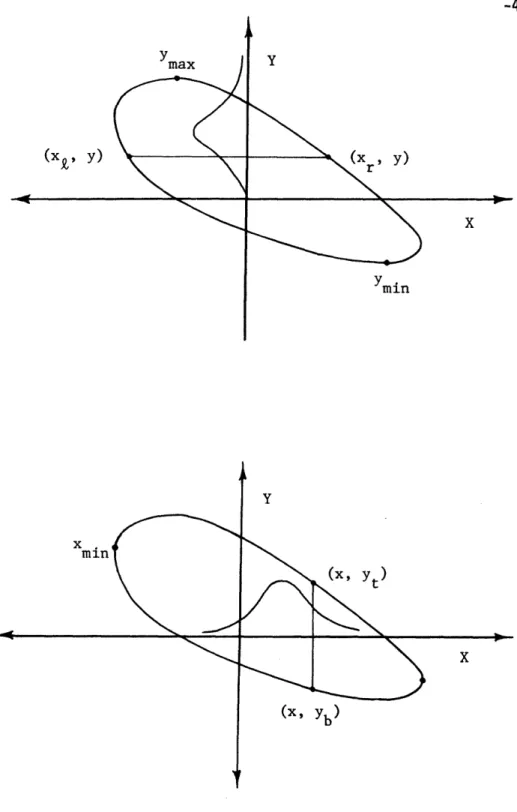
Also, we must consider the form of the boundary in order to write an

explicit result. Let us make a slight notational change at this point (to

reduce multiple subscripts). Instead of labeling the load variables for

loads 1 and 2 by sl and s2, simply call them x and y, respectively. There

are then 8 important points on the boundary to consider. These include

the extrema, Xmax' Ymax' Xmin' and Ymin' along with the intercepts xiV Xir' Yit, and Yib' All of these points are illustrated in figure 2.2.

ymax (XN, Y)

x.

_min

Figure 2.3: Integrations involved in the two dimensional modified square wave formulation.

1 -g -

L

-41-two paths from Ymin to Ymax' running to the left and right, containing

xiR and xir, respectively. Denote the ordinates relating to a given value

of y as xQ and xr, respectively.

So, using this notation, for a given value y, the probability of

being within the safe region is:

P{Safey} = F'l(r) - F'l(x) = P + ql[Fl(Xr ) - Fl()] (2.2)

Unity minus the right hand side of 2.2 is the probability of being out of

the safe region, given y. Since an outcrossing event involves the

transi-tion from a safe to an unsafe state, and recalling the independence of

successive renewals, l+ is:

V1+ = V1 max{pl+ql[Fl(r)-Fl(X ()]}{ql-ql[ Fl(xr)-Fl()]}dF'2

(y )

(2.3)

Ymin

Accounting for the probability P2, equation 2.3 becomes:

v1+ = Vlql P 2{l + ql[F1(Xr) - F₁(X9)]}{1 - [F₁(Xr) - F₁(X)] + lqlq₂

[max p q[ ()

I

Ymin

where f2(Y) now relates to the p.d.f. of renewals of load 2. Considering

a symmetric result for load 2, the final (total) result is obtained:

V+

= VlqlP

{pl +

ql[F

(x

-

F

(xk)]}{l

-

[F

(xr)

-

F(X)]}

Ymax

+

vlqlq

J

{Pl+q[Fl(Xr)-Fl (X)]1{1-[FI(xr)Fl (X)]}f2(Y)dy

p+q2[F2(t)-F2(b)]}{1-[F2(Yt)

Except for extremely simple cases of little practical interest, equation

2.5 must be evaluated numerically. The form of these two integrations are

indicated in figure 2.3.

2.2 Outcrossing Rate Results for Gaussian Processes

As mentioned previously, the results outlined in this section are

taken from reference [40]. Only slight changes in notation to resolve

cer-tain conflicts with other results have been made.

The general formulation is as follows. Let X(t) be a stationary,

con-tinuously differentiable process with n components, and n be a region in

Rn , defined by:

= {X: g(X) z (2.6)

That is, Q is the safe region defined by the function g.

Analogously with upcrossing events of scalar functions, a sample

func-tion (t) is said to outcross the boundary B at a time to if x(to) is on

B and:

xn(to) = (to ) ·-(to ) > (2.7)

-43-direction towards the exterior of . Intuitively, this means that at t,

the sample function is just on the boundary B, and has an outward

velo-city.

The approach used to find the outcrossing rate is a generalization of

Rice's argument [34]. It is expressed as:

+

I

f

B9 o Bo

where E[-] denotes a partial (or positive tail) expectation.

We will study a particular class of cases. First, assume that we

re-strict ourselves to stationary Gaussian processes, then X(t) and Xi(t)

are independent. Further, if we assume Xi(t) and Xj(t) to be independent,

i j, it also follows that

j(it)

2.8 becomes a constant independent of x:

E[RnX = x] n] := (2.9)

So, 2.8 becomes simply

+ EO[ ]f(B) (2.10)

where f(B.) is the probability density that X(t) is on the boundary at any

given time t.

Using the above assumptions makes a tractable equation for polyhedral

regions in Rn possible. First, reduce all coordinates by dividing each

component x_i through with the appropriate standard deviation aoi. Let the

with a unit exterior normal i.. The jth component of this normal is

de-noted here as nij. It can be shown that for this case, we may write the

density f(Bi) as:

f(Bi) = 4(ri) n-(B i ) (2.11)

where r_i is the distance from the mean point E[X] to the face B_i and (ri )

is the standard normal density evaluated at this distance. Further, On-l

(Bi) is the integral over Bi of the conditional density of X given that

X is on the (infinite) hyperplane of which Bi is a part. This is in the

form of an (n-l)-dimensional standard normal density with its mean at the

orthogonal projection of the mean E[X] on the hyperplane. This reduction

of dimension is particularly useful in the solution of two dimensional

problems, such as illustrated in figure 2.4.

Further consideration of face B yields another useful result. The

partial expectation for this single face becomes:

0

_E[nni

_l

₌

_(2.12)

where

2 n 2 2

ani j nij ajj

j=l and where

a2 Var(Xj)

that is, the variance of the jth component of the derivative process.

Application of equations 2.10, 2.11, and 2.12 now leads to the desired

lx

x

oc)

v+

i

f(B

)

nijajj

(2.13)

This is simplified further if attention is focused on the two

dimen-sional problem. In this case denote the components of ni as:

cos P n = _i

sini

J

and let 0i be the point on Bi closest to the mean E[X]. Then, Bi may be

split into two segments, from each vertex of Bi to Oi, as illustrated in

figure 2.5 (unless 0i is itself at a vertex). Let the algebraic distances

from the vertices of Bi to 0i be cli and c2i > Cli. Using these symbols,

equation 2.13 becomes:

1 m 2 2 2 1/2

+

_{+ - 2 i[}

2

_c2i)

21

_-

_(Cli)](a

li

_lCOS2

sin*)

exp(-r/2)

(2.14)

i

+ o2sin2~i) exp

This is the result of this section that is used later in this chapter to

actually calculate outcrossing rates.

We would like to use these results to study the modified square wave

process. However, to apply the result 2.14, we must supply stochastic

process information in the form of a₁₁ and 22. These parameters have no

direct analogues in the square wave process, since the derivative of the

square wave process does not exist. Yet, we may still attempt to achieve

comparable results by selecting all and a2 2 in some reasonable way. We

choose to do this by matching the mean rate of crossings of the mean level

-47-wave and Gaussian process formulations. For process 1 and the modified

square wave formulation:

2 2 2

: [Pl+qlFl(p)][ql-qlFl(p)]vl = [Plql+(q-Plql)F 1 )- q 1 1() (2.15)

Assume F₁(P) to refer to the mean of a normal distribution; then, it is

simply evaluated as 0.50. So, equation 2.14 becomes:

+ = (0.50 plql - 0.25 q )vl (2.16)

Use equation 2.13 with m = 1, i = 0, and (ci2 ) - (cl) = 1, to account

for an infinite straight line parallel to the x axis. With r = 0 to place

this line through the mean:

,+

(2.17)

Equating the right hand sides of 2.15 and 2.16, we get:

all = r(pl q l - 0.50 q)vl (2.18)

A similar result holds for process 2.

All of the mathematics necessary to this chapter are now at hand.

The following sections will deal with their application.

2.3 Case Studies: Reinforced Concrete Columns

Let us consider an example of a reinforced concrete column subject to

wind, live floor, and gravity dead loads. Assume the structural

interac-tion defined by equainterac-tion 1.9, but with L replaced by D + L. Treat D as a

constant in any particular case, a nominal (mean) value in the same sense

Less explicitly, the same end could be sought by raising the mean live

load, ;1 L' by an appropriate amount. However, the chosen approach has the

advantage of limiting the variability in the floor load to that actually

imposed by the live load process, therefore leaving the dead load both

de-terministic and constant in time, as it is commonly assumed to be.

Flexi-bility in choosing a dead to live load ratio is also maintained.

Consideration of random (though constant in time) dead load is

concep-tually straightforward. Equations 2.5 and 2.14, for either the jump or

continuous process formulations can be viewed as conditional results, given

a particular value of dead load. In each case then, replace the left hand

side, v+, with +ID. Assuming the dead load to be independent of the other

load processes, denote its distribution as fD(s). Then:

0

is the true mean rate of outcrossings, accounting for random dead load.

We shall explore this example three times. Each particular

combina-tion of an interaccombina-tion diagram and a matrix [C] will be referred to here

as a study. Each study will consist of at least three cases, which here

refer to sets of parameters characterizing the individual load processes.

The purpose of these studies is twofold. First, we shall examine the

be-havior of equations 2.5 and 2.13 by comparing the rates obtained for

dif-ferent cases. Then, we shall proceed to the main tasks of finding out

whether and how a failure boundary may be linearized.

2.3.1 Parameter Selection

-49-that may be encountered in practice, as far as possible. Interaction

dia-grams used here are from a paper dealing with column strength [18], and

may also be found in reference and text books, such as [41].

These diagrams have been presented in nondimensional form, based on

ratios of parameters. Parameters that have not been previously introduced

here are listed below:

e = ratio of ultimate moment to ultimate axial force, Mu/Pu

b = section width

h = total section depth

eh = depth between reinforcing layers

fc = concrete (crushing) strength

and A f

sy

As = reinforcing steel area

f = yield strength of reinforcing

Geometrical parameters are illustrated in figure 2.6.

Since the columns are symmetric, each interaction diagram may be

re-flected about its vertical axis. This describes behavior in the region of

(positive) axial force and negative bending moment. Furthermore, assume

no net tensile strength, therefore restricting each diagram to the region

of positive axial force. This convention serves to close each diagram

in-to a convex polygon.

pre-

*00

. I

-51-sented at the beginning of each individual study, along with the reasoning

behind their selections.

Load parameter values that define individual cases were suggested in

part by McGuire's report [29]. Floor live load was modeled as the

"sus-tained" live load in the report. To represent a building without

vacan-cies, p was chosen as zero. Also, the renewal rate of the live load

pro-cess was chosen as vL = 0.125 (per year), the value used in the report.

Finally, a value of 57% for the coefficient of variation of the live load

was used in the report, and is used in most cases here.

Judgement had to be excercised in the selection of reasonable values

for other parameters, however. For the dead load D, values of 150, 100,

and 75 (lbs. per ft.2) were chosen to represent normal, lightweight, and

very lightweight construction, respectively. Dead to mean live load

ratios of 3:1 or 2:1 were used. The parameter Pw was chosen in all cases

as 0.9977. So, with vw = 2190, we have a mean rate of

(1 - 0.9977)2190 = 5 storms per year. With Vw = 1314:

(1 - 0.9977)1314 = 3

storms per year is the mean rate of arrival. Further, the storms have

mean durations of:

(1/2190)(8760 hrs./yr.) = 4.00 hours (1/1314)(8760 hrs./yr.) = 6.67 hours

in these respective cases, or a total of 20 hours per year, either way.

stan-dard deviation of 5.0, this corresponds to coefficients of variation from

14% to 50%.

The values used for the stochastic load process parameters are

pre-sented in tabular form with each study.

2.3.2 Computational Procedures

Before proceeding, the computational procedures necessary to carry out

the case studies will be briefly discussed.

Equation 2.5 for modified square wave processes has been evaluated

using Simpson's rule by a Fortran computer program. We shall refer to this

program as the Outcrossing Rate Program, O.R.P. for short. A listing and

a summary of O.R.P.'s input formats is given in the appendix.

As input, O.R.P. accepts the following:

1. The matrix [C].

2. The column interaction diagram, in a point-by-point form.

3. The parameters vw, , w' aw, VL, L, 0L, and D.

Furthermore, either normal or gamma distribution functions can be specified

for either load process.

As output, O.R.P. yields:

1. The transformed interaction diagram in terms of wind and floor loads,

and the extrema pertaining to this diagram.

2. The four paths from extrema to extrema, as illustrated in figure 2.3,

and the x and y axis intercepts.

3. The value of the mean outcrossing rate (including the individual

contri-butions due to each load process as well as the sum).

-53-boundaries. By specifying the identity matrix for [C], such boundaries may

be input directly; that is, the transformation will not change the diagram.

This boundary should not take the form of vertical or horizontal lines,

such as the axes, however. Either zero or infinite slopes along portions

of the failure boundary may confuse the routines that search for extremum

points and result in invalid output.

Equation 2.14 for continuous Gaussian processes may be evaluated by

hand. When doing so, it is helpful to proceed in the following manner:

1. Reduce the coordinates of the transformed interaction diagram (from

O.R.P. or hand calculations) by division by the appropriate standard

de-viations; so the points W* and L* become W*/aw and L*/aL.

2. Find the reduced means, corresponding to pw/Ow and (D + L)/aL.

3. Find the points Oi, and the distances to the mean, ri .

4. Find the distances cli and c2i, and then use standard tables to evaluate

(cli) and (c2i).

5. Having tabulated all of the above, compute the crossing rate due to each

segment, and then sum all of these rates.

Step 3 amounts to an elementary excercise in analytic geometry.

How-ever, for the purpose of checking for errors, it is useful to make plots or

geometric constructions as one proceeds.

2.3.3 Study 1

The first column chosen has a rectangular section with = 0.90 and

pp = 0.50. This section is deep and well suited to bending, and moderately

reinforced. Assume the following interaction matrix:

6.0 x 103 1.5 x 10-4

(all in units of ft.2/lb.). This corresponds to a situation such as

fol-lows. Most of the axial effects are due to the vertical loading and most

of the bending to the wind, but there are significant effects due to the

off diagonal terms. Column eccentricity translates vertical loads into

bending effects. Wind load adds to axial forces, such as may be the case

when the column is not near the centroid of the building.

The interaction diagram, showing the mean load effects for cases A, B,

and C as well, is shown in figure 2.7. After it has been mapped to load

space, it assumes the form of figure 2.8. Since the off diagonal terms of

[C] are about an order of magnitude less than those on the diagonal, the

diagram has not been badly distorted.

To facilitate evaluation of v+ by equation 2.14, the coordinates on

the latter diagram were reduced by division with ow and oL . The resulting

diagram is shown in both figures 2.9 and 2.10. It was noted that the

seg-ment closest to the mean made the greatest single contribution to the

out-crossing rate in each case, with the next largest contribution owing to an

adjacent segment. This suggested that linearizations of the failure

sur-face be made by simply extending the segment closest to the mean in any

given case. This minimization of r corresponds to the criterion suggested

in the papers by Hasofer and Lind [25] or Ditlevsen and Skov [17]. Figures

2.9 and 2.10 also illustrate the linearizations.

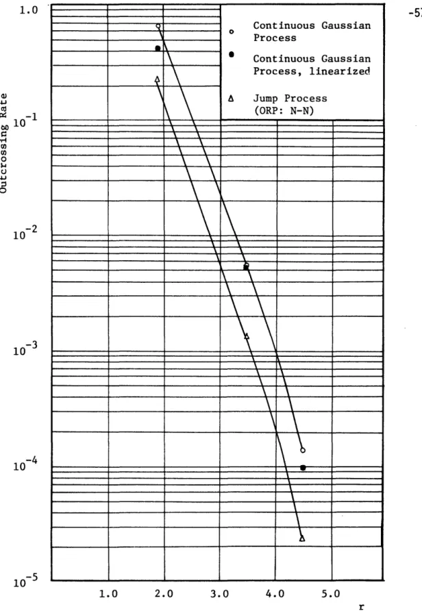
Outcrossing rate results for the different methods are plotted versus

r and shown in figure 2.11. The top curve shows the results of equation

2.14, and the points below it the results based on the same continuous

pro-cess but with the failure surface linearized. The lower curve shows the

a)

0U

.

a

O

, O 0 CN -0 :3 o:~ O '-4

:

c

c

-56- -'

0

1.0 4J 10 10 -3 10 10- 5 10

1.0

1.0

Figure 2.12: Linearizations of the jump process, study 1.

t, 0 U) (U)

0

1-2

-59-on each load. All of the plots are smooth curves that are almost straight

lines on semilog paper. The curvature that does exist might be attributed

to the fact that the tail of a normal distribution decays at a greater than

exponential rate.

The linearizations were in error by 37%, 4.8%, and 30% for cases C, A,

and B (listed with respect to increasing r). All of these errors are in

the form of underestimates. This is due to the nature of the failure

dia-gram; it is convex, and therefore, the linear segments are always on or

be-yond its boundary. No relationship between the magnitude of the error and

r has been found in this or in the other studies. Instead, the reason case

A gave the least error seems to be that it is nearer the center of the

seg-ment (that A and B are both closest to) and this segseg-ment is much longer

than the closest segment to C. However, using this concept does not help

to formulate an objective criterion to predict or judge the magnitude of

the error.

Then, the jump process was used to find the outcrossing rates for both

the full and linearized boundaries, assuming gamma distributions on both

load processes. These results are plotted on figure 2.12. Note that the

results based on the full boundary now fall on a straight line, due

appar-ently to the nearly exponential nature of the gamma tail. However, the

er-rors caused by linearization have become 28%, 12%, and 30% respectively.

The only apparent conclusion is that for these cases use of gamma

distribu-tions made the error less sensitive to the position of the mean point than

use of normal distributions.

All of the results are summarized in table 2.1.

o o o

o o 0

U)

0 0

0

o

o

c) C) c)

r

a

c

%"

0

o

'a

0

0 z

-*- XX

:

0 0

c,