"Tor~~~~~~~ ~~~~~~~~~~~~~~~~~~~~~~~~~~~ -er.. -:- :~~~~~~~~~~~~~~~~~~~.. ~v ~-~!-::~!i r '.:;:,~::;~ ~~:~ i ~ ~
r:;.
.
,_:
n S!
:
EA C
?
:?
: ~
E S
fj'V~
~ ~ ~ ~ff
~ ~ ~- fE.0.jffE-ffi 0.
~,:-0 -,: .:,e:.:St0
~~~~:g:I:.
i 3:: '
<-;E
:4:
.~I- .:-00:
pae
wring0
:0
f0:
-:
:;
0000:00 :X; -: - -:4 ;
.
t_:: :-: ·. - : ~; .: ;, "': f f 'C00000ff 0 0 ;f~~~~~~~~~~~~~~~~~-' ' ~': ~ : ;00 77 ! 00: ~" ~-.:~~':' S; ? : '. ~ -i ~ ~ ~ ~ ~ '~~- ' :', ,,: '~; .,-i'.;'' '~ .~.( . , ' ,' ' ' ."!~ ? : ,- ,'' ~: f -~ ~-' ~;, : - . , ' i 'L-- .'_' ', ' ,.',.''.:~ , , _'_'''', 'i ,,' i'- ' .; '_ ' '. ' - ' - , .. .''" '"'' 0 : ' " ' ' ' ' .',..' '.. ' . . , '.',-rS'T t00 'V 00 f 0 g , 0| ; 0000 00D ff E 0 0 0 z 00 tuffff ; ' ; f t; f t f0 ; 0 E'V'D f ;f 0 V ' S ' f 0 0 0''R0 W~~~~~~~~~~~~~~~~~~~~~~~~~~~~~~~~~~~~~~~~~~~~~~~~~~~~~i!:
i`
-...
:. .
-. ·-.··
;
il-··r· · · ; -i · ··-... .-i ;e .; .: ···. · -· . -;--:· "--· ;· .:·.. I .··. -:-'·· ·r. 5. : i; ' ;·- :·-.·- ' I : I ;· '' ··· , '· ·- · ·An Analytic Approach to a General Class of G/G/s Queueing Systems
by
Dimitris Bertsimas
V
An analytic approach to a general class
of G/G/s queueing systems
by
Dimitris Bertsimas
Department of Mathematics and Operations Research Center Massachussetts Institute of Technology
Rm 2-342, Cambridge, Mass. 02139, USA Abstract
We solve the queueing system (QS) Ck/Cm/s, where Ck is the class of Coxian probability density functions (pdfs) of order k, which is a subset of the pdfs that have rational Laplace transform (R). We formulate the model as a continuous-time, infinite-space Markov chain by generalizing the method of stages. By using a generating function technique, we solve an infinite system of partial difference equations and find closed form expressions for the system-size, general-time, pre-arrival, post-departure probability distributions and the usual performance measures. In particular, we prove that the probability of
n customers being in the system, when it is "saturated" (n s) is a linear
s+m-1
combination of exactly ( s ) geometric terms. The closed form expressions involve a solution of a system of nonlinear equations that involves only the Laplace transforms of the interarrival and service time distributions. We con-jecture that this result holds for the more general model GIRls. Following
these theoretical results we propose an exact algorithm for finding the system-size distribution and system's performance measures, which has an algorithmic complexity of O(k3(+' s)3). We examine special cases and apply this method for solving numerically the QS C2/C2/s and Ek/C2/s.
Acknowledgments
I would like to express my appreciation to my advisor Professor Amedeo Odoni for his encouragement and support throughout the course of my Master thesis, a part of which is this paper. I would also like to thank the Mathematics department of MIT for awarding me an Applied Mathematics Fellowship.
Introduction
Throughout this century queueing theory has been studied thoroughly, but still many problems remain unsolved, in spite of the effort and intelligence devoted to them. Among these problems, the analysis of the G/G/s queueing system(QS) has survived the "attacks" of many excellent mathematicians, obviously due to its inherent complexity.
In this paper we generalize the method of stages, introduced earlier in the cen-tury by Erlang and combine it with a generating function technique to achieve the solution of the general class of problems C,/C,/s, where C, is the Coxian class of probability density functions (pdf's) with rational Laplace transform.
A brief critical presentation of alternative solution methods
When it comes to exact solutions of multi-server QS's, the more one departs from the assumption of exponentiallity, the more thorny problems become (especially if this happens for the service time pdf or, worse, for both the service and arrival-time pdf). Thus the only solution approaches that have up-to-now been established as supposedly "general-purpose" are, in chronological order of appearance:
1. The method of succesive exponential stages 2. Complex variable theory
3. Imbedded Markov chain
4. Inclusion of supplementary variables
We believe that the following very short commentary on the application of these solution approaches to multi-server models assesses fairly their inherent potential to produce theoretical and, especially, exact numerical results (which should usually be their ultimate goal).
The Imbedded Markov chain method
In the past decade it was mainly Neuts and a number of other authors who, by exploiting the phase-type (PH) distribution and by developing the powerful but still "esoteric" formalism of the associated matrix-analytic methods and algorith-mic approaches (as presented in Neuts (1981), (1984)) have managed, by bridging" this method with the method of stages, to considerably extend its potential. Yet, for multi-server systems with non-exponential service times the relevant solutions (although providing qualitative insight) lead to major dimensionality problems. For the EkI/Cm/ model this approach requires the solution of a non-linear matrix
equa-tion involving matrices of order mn, so that (even for C2) Bellman's dimensionality
curse precludes the derivation of any exact results (except for very small values of
s).
The inclusion of supplementary variables method
Despite the initial great expectations concerning its capabilities, the method has been used for multi-server systems in a limited number of analytic investigations (not to mention numerical implementations). In the last decade Ishikawa (1979) tried to tackle the G/E,m/s system through this method, but he restricted his at-tention to the G/Es/3 system. In parallel, Hokstad (1978) started his investigation of the MIGIs system by writing the associated equations, which he managed to
"solve" in Hokstad (1979) but only for the M/R/2 case, where R is the class of
distributions with rational Laplace transforms. Then he specialized to the M/C2/2
(and thence to the M/E2/2 and M/H2/2) producing some limited results. In his
next (Hokstad (1980)) paper he uses a "refined and modified" version of his previ-ous analysis, which he claims to be in principle applicable to the general MI/CIs model (but with complicated results). He was compelled to restrict attention to
the M/C2/s and (after various simplifications) to present very limited results for
M/C 2/s QS. Both the above approaches are complicated, while Hokstad's general
algorithm (according to van Hoorn (1983), p.29) is numerically unstable and not reliable for higher s values.
The complex variable theory method
Pollaczek's method (Pollaczek (1961)) is by its structure limited to First-Come-First-Serve (FCFS). The method was exploited by de Smit, whose venture started with some abstract results for the G/G/s QS (de Smit (1973a)), which were then specialized to G/M/s (de Smit (1973b)), and continued with a method of approach for G/H,/s (de Smit (1983a),(1983c)). Yet, this approach needs deep arguments from complex variable theory, leading to a numerical solution in the G/H2/s case, but with a high computational complexity which is proportional to s6, to be
com-pared with O(sS) of our method.
The method of succesive exponential stages
Erlang's ingenious method of stages has for some time been neglected, obviously because of researchers' concern about the fact that it does lead to systems of equa-tions which usually are complicated (but certainly not looking more formidable than those of the previous methods) and become almost intractable if one attempts to tackle them directly by various seemingly powerful techniques. For example in the
EkA/E/Is case this intractability is apparent both
1. In many of the earlier attempts at an exact solution via multidimensional gen-erating function techniques (see, e.g., the annotated, but not totally complete, bibliography by Ovuworie (1980))
2. In Yu's (1977) ambitious theoretical treatise, via an intricate partitioning of the system-states and an exploitation of the cyclic structure (exhibited by the corresponding transitions) through the use of polynomial matrices.
the computations necessary for the derivation of numerical results involve the nu-merical expansion of such matrices, which is still an enormous task even for mod-erate values of k, m and s.
The above mentioned attitude is reflected in the comments of Kleinrock (1975), p.146-7. But on the contrary, and more in line with Cohen (1982), p.346, we believe that this method with a proper solution strategy, like the one presented in this paper, is so powerful that it is difficult to overemphasize its importance for the exact solution of intrinsically difficult multi-server queueing systems.
On the class of Coxian distributions C,
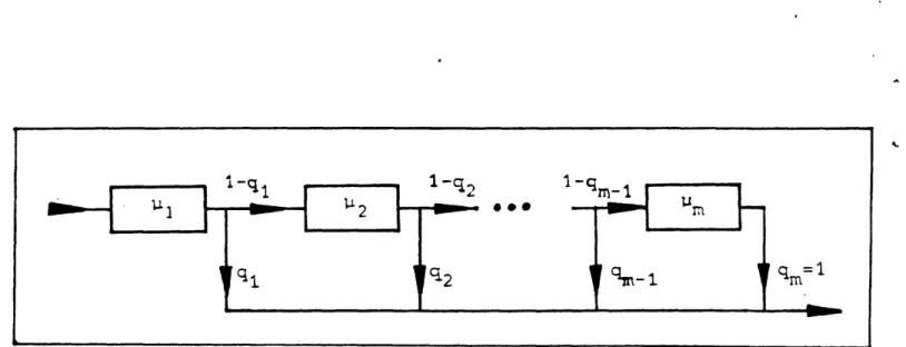
The general Coxian class C, was introduced in Cox's (1955) pioneering paper and is clearly presented in Kleinrock (1975). It is remarkable that even if we permit transitions from a stage with rate ti to a stage with rate uj in figure 1 we do not obtain a new class of distributions. We can still formulate this situation with a C, distribution with different transition rates. The salient feature of the class C, is its high versatility (see e.g. Neuts (1981), Whitt (1982)) based on its ability to:
1. Generalize well-known distributions such as the exponential, the hyperexpo-nential and all the forms (i.e., special, general, weighted, compound, etc.) of the Erlangian.
2. Be dense in the set of all probability distributions concentrated on (0, oo) and thus to be able to approximate a general pdf.
3. Permit coefficients of variation V2 greater than 1.
Figure 1: The C, class of distributions
into exponential-stages, so that we can use a powerful modification of the method of stages.
Our result
Our result generalizes the well known G/G/1 theory to multi-server systems in a natural probabilistic way. Our approach, in comparison to the methods used earlier in the evolution of queueing theory is easier to grasp and easier to implement. More importantly, it leads to an algorithm of relatively low order of complexity. On the other hand, in comparison to the purely numerical methods of Allen, Andersen and Seneta (1977), Takahashi and Takami (1976) (which was recently specialized by Groenevelt, van Hoorn and Tijms (1984) for the solution of the much simpler models
M/H 2/s, M/E1,2/s, M/E1,3/s) and Seelen (1986) the present approach offers full
qualitative insight by providing closed-form expressions, which apart from their computational value, are also of theoretical interest. Furthermore, our solution strategy leads to an exact waiting-time analysis under FCFS, which is going to be presented in a forthcoming paper.
From an algorithmic point of view we propose an O(kS('+-l)3) algorithm for the calculation of the performance measures and the probability distributions of this QS, which for a given m is polynomial in the number of servers. In other words, we prove that for a given service time pdf the solution of the related queueing problem is polynomial in the number of servers.
To test properly the potential and reliability of this method, we prepared com-puter programs for the numerical solution of the QS's Ek/C2/s, C2/C 2/s . These
exact results are in full agreement with all others available in the literature and can be exploited for the always desirable sensitivity analysis and comparative evaluation in the continuously active areas of
1. approximations for multi-server models (e.g. those on the M/G/s QS recently reviewed by Tijms, van Hoorn and Federguen (1981), Sze (1984)).
2. inequalities, bounds and stochastic order relationships on both of which there is a rapidly increasing literature.
In the next section we formulate the model as a continuous time Markov chain using the method of stages. In section 2 we apply a generating function technique for solving the difference equations that describe the system. In this section, which is central to the analysis, we combine results of the complex-variable-theory method developed by Pollaczek (1961) and de Smit (1983a) with results of the present paper to prove what we call the "separability property": The probability of n customers
(n > s) being in the system is a linear combination of ( s ) geometric terms. In
section 2.5 we examine as special cases the QS's Cn,Cm/1, C,,IMs, Ek/E,/Is and
En/C2/s.
The derivations of closed form expressions for the system size probability distri-butions and the usual performance measures are outlined in section 3. In section 4 we include some computational and complexity considerations, while the final section contains some concluding remarks and open problems.
1
Formulation of the model as a continuous-time
Markov chain
We shall examine, henceforth, an s identical-single-waiting-line QS with interarrival and service time distributions of Coxian type of order k and m respectively. There are no restrictions in the queue discipline except that no server can be idle if the queue is not empty.
1.1 Probabilistic interpretation of the QS
To analyse the model we conceive of the arrival process as an arrival timing channel (ATC) consisting of k consecutive stages with rates
A
1, A2,..., Ak and withproba-bilities P,P2,..-.Pk - 1 of entering the QS after the completion of the 1st, 2nd, ... kth stage. We remark that as soon as a customer in the ATC enters the QS a new customer arrives at stage 1 of the ATC. For the service time distribution we consider as above a service timing channel (STC) consisting of m consecutive
stages with rates Al, I2, .., Arm and with probabilities ql, q2, ... , qm 1 of leaving the
system.
1.2 Notation
For the steady-state we introduce the random variables 1. N The number of customers in the system.
2. N- The number of customers seen by an arriving customer just before his arrival.
3. N+ The number of customers seen by a departing customer just after his departure.
4. Ra A The number of the ATC stage currently occupied by tomer.
A
5. Rj - The number of customers being served at the jth 1, 2, ... ,m).
6. R - The number of customers being served at the jth 1, 2,..., m), just before the arrival of an entering customer.
the arriving
cus-STC stage (j =
STC stage (j =
7. Tq - The waiting time of an arriving customer.
For simplicity of notation we introduce the vectors of random variables
and also we will use the notation:
a,
A (0 1,o0..,) , ,... , a(s,m) A ( +s )II = a meaning that E=l ij = 8.
With the above definitions the system can be formulated as a continuous time Markov chain with infinite state space:
{(N,RaR,...
Rm),
N = 0,1,..., Ra = 1,2,...k, R = min(N,s)}j=1
where the states with N < s (i.e., the states with at least one server free) and N > s (or all servers busy) will be termed "unsaturated" and "saturated" respectively.
We now introduce the following set of probabilities, some of which will be used in later sections. Pn,Ij Pr{N = n, R. =, = P-- Pr{N = n,R-
=
i} n,% Pn-Pr{N = n} Pn Pr{N- = n} P+ Pr{N+ = n} We also define:f;. (0), f (0) A The Laplace transform of the interarrival and service time
distri-butions respectively.
The mean interarrival time. A The mean service time. pz = The traffic intensity.
1.3
The equations
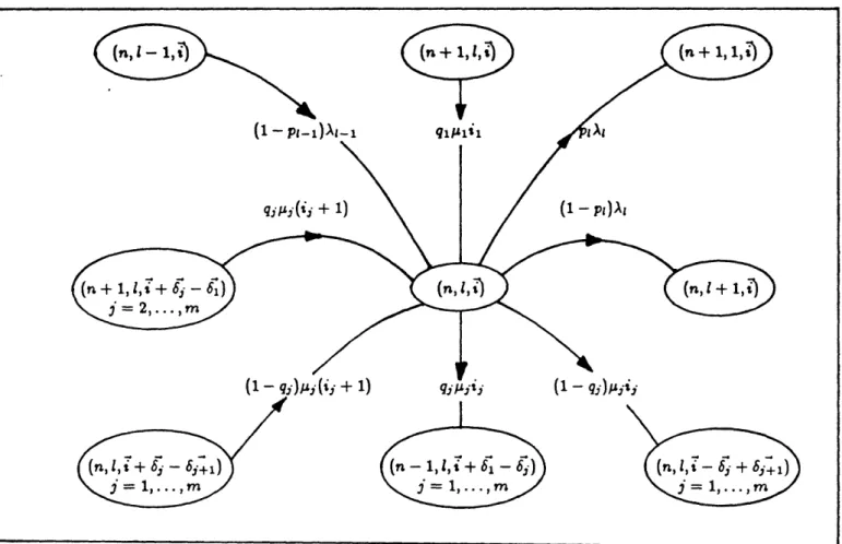
After drawing the rather complicated state-transition diagram in figure 2 (for the case I = 2,..., k, the case I = 1 is similar) we write down the following system of
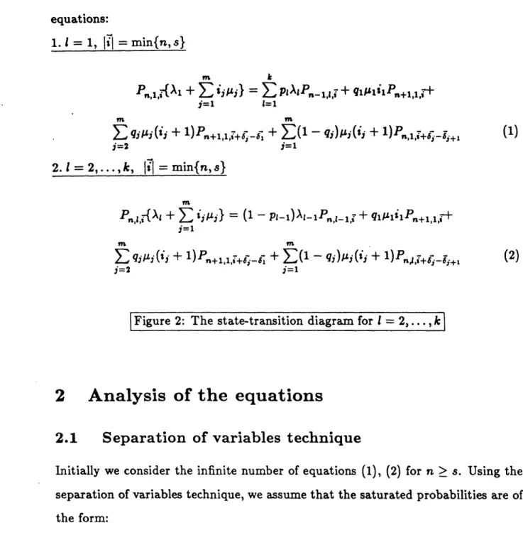
equations: 1. I = 1,
Iil
= min{n, s} k :E l=l m nl{+ ij} = j=1 m E qpi(ij + i)P.+j,',+i_; + j=2 2. = 2, .. ., k, = min{n, s} Pl.,,L + E injj} = (1 -:=1 j (ij + 1) Pn+,1,'i6jt j=2 (1) -(1- qj)j(ij + 1)P,,,i+sji+ j=l PI-1)X-1P,-1 1, + qltjlilPn+l,l,i-+ Z(1 - q)tAj(ij + 1)P,,i+-i j=1 (2)Figure 2: The state-transition diagram for I = 2,..., k
2
Analysis of the equations
2.1
Separation of variables technique
Initially we consider the infinite number of equations (1), (2) for n > s. Using the separation of variables technique, we assume that the saturated probabilities are of the form:
Pn,,i = Di Rr w" n>s
with the obvious conditions
R. =O for
m
E ij S
j=1
91CLA1'Pn+1,1,&-Then from equations (1),(2) for n > s we get:
1. 1=1, iiI = s
m
D1R-{A1 +
j=1
iiij} =- plAIDIR; + wqAilDR-+
W =1
+ 1)DIR+f-_ + -(1- qi)si(ij + 1)D 1R+-i_ +
j=1
DRA,I + E ijj} = (1 - l-,l)
j=1
XI-_lD-lR; + wqllzlilDiR+
m sm
w E qijj(ij + 1)Di Ri-+j;._ + Z(1 - qj)Lj(ij + 1)DIR;Z
j=2 j=l
Then (4) can be written:
R{DIA - (1 - p-l)Al_,D_}= Di{wqllilR,-+
m m w q qjj(ij + 1)R-+_j. + (1 - qj)Aj(ij + 1)R+fs_6+ i=2 j=1 m - RZ- ij=j} j=l
Using the usual "separation of variables technique" arguments we demand that
DlAl - (1 - Pi-I)A-lD-1 = -xD 1 I = 2, ... , k wqllilRt + w n qilj(ij + 1)RZ-+j E6 + Z(1 j=2 j=1 - qj)Aj(ij + 1)R-+,-_i+-m R; Z ijs = -R;,
It
= s j=1for some constant x that depends on w. Solving (5) we find that
DI=D1 I = 2,...,k
r=Substituting (6) we find the relation between x and w.r+(7) to (3) and using
Substituting (7) to (3) and using (6) we find the relation between x and w.
= pA I 1=1x + A r= (6) (7) (8) (1-pr)Ar = f.() X + A\r w ~ qjAj(ij j=2 (3) (4) (5) 2. 1 = 2 ... , Ik, jil =
(the product for = 1 is defined to equal 1)
Equations (6) form a linear homogeneous system of a(s, m) with a(s,m) un-knowns. The only way for a nontrivial solution to exist is for the determinant of the system to equal 0, i.e.
Det(w)= 0 (9)
2.2 A generating function technique
From (9) we can in principle find the roots w inside the unit circle that satisfy (3), (4). Since the numerical determination of the roots w is of extreme computational complexity, because of the large dimensions of the determinant, we will use a method based on generating functions in order to find the roots w. For this purpose we introduce the m multivariable generating function:
u( ) = R z ,1 .. , i= (i ... i), z = (Zl ... zm)
Ilq-.
Multiplying (6) by z' ... z. we get the following partial differential equation of first order:
dU
az (izjz - wz - (1 - qj)zj+l) = xU(z-) (10)/=1 z
For the derivation of (10) we have used the identities:
zau() - E Riz ... z
Zr
a(2-)
R(ij+
1) z ' , r=1,j +1az
j T
The new idea we introduce in this section, the exploitation of which is presented in section 2.3, is that the solution of (10) combined with the requirement that this solution must be a multivariable polynomial, will lead to the determination of the roots w.
2.3
The method of characteristics
Our goal is to solve (10) which is a linear partial differential equation (pde) of first order involving m variables. We will use a well known method, the method of characteristics, from the theory of pde's in order to solve it. Then we form the system of ordinary d.e's:
dzl dzi
(1 - wql)julzl - (1 - ql)AllZ 2 --wqjjzl + ZjZj - (1 - qi).LjZj+l
dzm dU(z
W=-Umz mZm = = dt
-WAmZ + .mzm ,X U(Z-)
(11)which can be written:
(12)
dz
= Amz
dt
where Am is the m x m matrix:
-wqlll + L1 -(1 - ql)11
-wq2A2 A2
-wqlAm,-I
--Wq1,Am
In order to solve the system . In the following proposition 1 Am satisfy. 0 -(1 -q2)2 0 0 0 M... m-1 -(1 -qm-l)m-0 ... 0 Am
(12) we must find the eigenvalues of the matrix Am we find the equation that the eigenvalues of matrix
Proposition 1
The eigenvalues of matrix Am are the m roots Oi(x) i = 1,...,m of the following equation:
(13)
fa.()f.(- (x)) = 1 Am
-Proof
We will prove (13) inductively using the following induction hypothesis: Induction hypothesis:
where
f.,, (0) the Laplace transform
.,
(0f)
f ().-IA,- I = (1 -
f,,(-6)) H=
1(Aj - 6)of the service time pdf with k poles
For k = 1 we have
IA, - I = -wqll + A1 - 0
But since ql = 1 , then
lA1- OI = (A - 0)(1 - wf;,, (-))
Assume that the induction hypothesis is true for k - 1. Then expanding the deter-minant At - OIl we take
k-I
IA, - OI = (k -
6)
IA,_1 - OI - wqk II (1 - qj)j j=lThen, using the induction hypothesis:
k
jAk - VII = (1 - wf,.,_ (-o)) (j
j=l k-i - 9) - wqAsk
1 1(1
- qj)j j=1 Therefore kIAk - OIl = I ( - 0){(1 - wf~',_,_ (-O))
-k
(1 - f., (-0)) Hll (j - 0) j=1
Therefore the eigenvalues of A, are the roots of the equation:
(1 - wf.(-6)) = 0
-W-- q:Ii -- " l (1 -Ii j)tily A~kt j l i=
-which combined with (8) gives (13).V
Therefore from (12) and (13) we find
m
Z = 1 ej(z ) t
j=l
(14)
where -[cl,, ,,j,.]T is the eigenvector of matrix Am corresponding to the eigenvalue Oj(x) . Also from (11)
U((t)) = Cet (15)
Since Cj is an eigenvector of A, its components C2,j,.. ., Cmj are multiples of cj
and thus
ciJ = ai,jclj, ali = 1
where aid can be found explicitly. Simplifying t from the equations (14), (15) and defining bj cj/C (bi are still undetermined) we find:
z bjajU (z-3 i = 1...m
j=l
and we find that:
1 ... 1 z1 1 ... 1
a2,1 ... a2,j-1 Z2 a2j+I ... a2,m
am,l ... amj- Zm amj+l .. am,m
I_(seI
.v.-bij U- (z- = (bl.iz + ... + bmz,)U.z
(--1 ... 1 1 1 ... 1
a2,1 ... a2j- 1 a2 j a2j+l .- a2,m
... a, a a ...
a,l ... amj- am, amj+l ... am,m
(16)
where bi, can be computed analytically from aij by expanding the determinants in (16). From (16), after solving with respect to U(z', we find that
U .2 = b (bljzl +-.+bmjz.) (j = M) (17)
We want to find a general solution of (10), which satisfies the condition that U() is a multivariable integer polynomial of zl,..., zm of degree s.
Raising (17) to some integer ij and multiplying these m equations we find:
U ( = K II (bl,,zi + ... + bmjz)' (18)
j=l
where K .
L
is an undetermined constant.Clearly (18) satisfies (10). In order for U(z) to be a multivariable integer polynomial of z of degree s we demand:
)=
=
=
1
ij =
ij Z
+
(19)
2: j=1 I I . ·- I L - . - ---- ---I I ITherefore, if the above conditions hold, we have found a solution of (10) that sat-isfies the "polynomiality" condition. Hence the generating function U(z that
cor-responds to the combination i = (il,... , m) is of the form:
m
U,-( =
K
II (bljz + ... + bjZ)'i (20)j=1
Let us summarize what we have shown up to this point. Our goal was to find the roots of the determinantal equation (9). For this goal we have defined the auxiliary generating function U(z) and we have shown that for every of the
a(s, m) combinations of the vector i, such that
il
= s (i= i = s), there existsa polynomial solution U;() of the form (20), if there exists an (wj) (and thus
a wi = f.(x)) that satisfies (19). The functions ij(z) which appear in (19) are
computed from equation (13).
In the next section we prove that for each of the a(s,m) combinations of the
vector i, such that il = s there is at least one root w inside the unit cycle.
Fur-thermore if p < 1, by using a result from the method of complex-variable-theory we prove that this root is unique and all the roots of (9) for p < 1 satisfy a nonlinear system of equations (see equations (21), (22) and (23)). Thus the use of the gener-ating function will enable us to completely characterize the equation that each root
w satisfies (note that each root w satisfies a different equation).
2.4
The basic separability theorem
From the results of the previous section we have to solve the following equation in order to find the roots w that satisfy (9):
+,() = i161(X) + i2 2(x) + ... + i,mO,() = X, i + 2 + + i... = .(21)
where j(z) (j = 1,..., m) are the m roots of the equation:
Since w = f. (x) we are interested in the roots z that satisfy the following equation
If.(x) < 1 (23)
In order to investigate the number of roots of (21) we prove the following theorem.
Theorem 2
If p < 1, for every of the a(s,m) combinations of , [i = equation (21) has at least one root x that satisfies (23).
Proof
First we prove that there are no roots x such that
Re{xz < 0
If Re{x} < 0 then from (21) there exists a j (1 < j < m) such that Re{Oj(x)} < 0. Then
lfW{J-Oj(x)}) I e i( )fT.(t)dtj <f jei(')tfT.(t)dt =
R
eR({'())tfT.(t)dt < 1
Therefore, combining the above strict inequality and (22) we conclude that since
f~.(x)f~,(-Oj(x)) = 1 then lf.(x)l > 1. Therefore the assumption Re{x} < 0
violates (23) and hence there are no roots x such that Re{x} < 0.
We now prove that for every combination i there exists a root z in the right half plane (Re{x} > O) which satisfies the system of equations (21), (22) using the fol-lowing fixed point theorem.
Fixed point theorem
Every continuous function f(x) defined from a convex, bounded and closed region into itself has a fixed point z0, i.e. there exists an x0 such that f(zo) = z0.
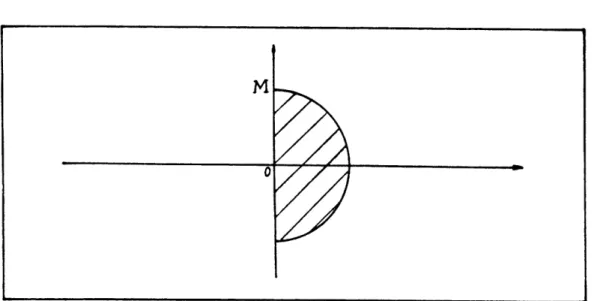
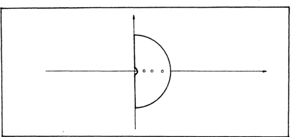
We will prove that there exists an M such that *(x) defined in (21) has a fixed point in the region DM {x : Re{x} > 0 , Ix < M}, in other words that there
exists a root x in the right half plane.
Clearly DM (see also figure 3) is convex, bounded and closed (compact).
Figure 3: Fixed point theorem in region DM
Also all functions ej(x) defined from (22) are continuous, since they are roots of a polynomial equation, where all coefficients are continuous functions of x. Therefore i(:x) is a continuous function, since it is a linear combination of continuous func-tions. In order to complete the proof that there is a fixed point it suffices to prove that there exists an M such that +,[(x) takes values in DM. From (22), we have
that for every j = 1,...,m Re{(j(x)}) 0, because if Re{(j(x)} < 0 then
f(-O
Ai(x)}l
- I 'ei(')tfT.(t)dtI < 1 AlsoIf;.
(x) I
I
|
SfT, (t)dt< 1
Then
IfT.; (X)If{-j()} < 1
and therefore (22) cannot possibly be satisfied. Thus Re{((x)} > 0. We now claim that there exists an M such that
IOj(x)I
< Ml -MIf not, for all M there exists a y such that [Oi(y)l > M1, that is Oi(x ) tends to
infinity as x - y. Since limjl_,.o f (x) = 0 , then from (22) in order for the product f(x)f,.(-Oj(Z)) to be non-zero, -(z) must tend to a pole of f(.). Thus
lim j(x) = i ,j=-,...,m
But since Oi(z ) is bounded at infinity; y is finite and
lim (z) = oo
which contradicts the continuity of
ej(z).
Therefore there exists an M such thatlei(x)l
< M and therefore from (21) (zx) < M, which proves that x-(z) is fromDM into DM and thus, since DM is convex and compact, has a fixed point in DM. Therefore we have shown that for every combination of there exists a root of the system of equations (21) and (22). Furthermore, if Re{xz > 0, x 0 then
If/(x) < 1. Yet, the solution x = is not excluded. In fact, for = (0,... , s) x = 0 is a solution to (21), (22). If there are two non-zero components ik, i of the vector , we can easily check that x = 0 cannot be a solution to (21), (22).
Therefore, in order to prove the theorem, we are led to the investigation of the roots for the m combinations of i where m -1 components are 0 and one is equal to s. Using Rouche's theorem we prove that when p < 1 then these roots are unique and non zero. Then equation (21) becomes
f(z)f;.
(--)
=We are going to apply Rouche's theorem in the region of figure 4. Then
1. Re{xz = 0 ( 0)
We easily get that If;.(z)I < 1 and Ifi,(-,) < 1, from where
If;(X) I < 2. Re{x > , Ij -oo
Then limljl, f(z) = ' and limll-. f .(-~) = O. Thus for
I1x
= L forsome big enough L and Re{x} > 0
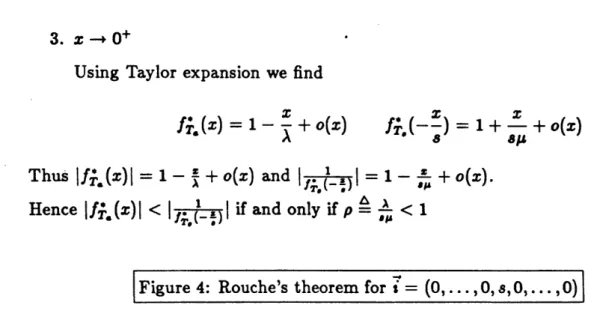
3. z-- 0+
Using Taylor expansion we find
f() ; =- X + o(X) f=
(
-- + + o(Z)Thus If.(x) = 1- + o(z) and I= 1 - + o(x).
Hence
If~.(z)I
<I;
I1
if
and
only if p-
<1Figure 4: Rouche's theorem for t = (0,..., , s, 0,..., 0)
Since in order to apply Rouche's theorem the functions f(z) and ( should
be analytic we must exclude from the region in figure 4 all the zeros of f,(-~)
(which coincide with the poles of ), points where is not analytic. But
in the vicinity of the zeros of f((-): tfu(x) < IJ. Z)I
,
i.e. the required strictinequality holds so we can apply Rouche's theorem in the region of figure 4 to find that (21) has m roots which obviously satisfy (23) since Re{x} > 0 . Since we have proved that there are no roots for Re{x} < 0 we conclude that if p < 1 (21), has exactly m roots which satisfy (23), for the m combinations of i where m - 1 components are 0 and one is equal to s. Combining the above result and the general proof that there exists a root for every combination of i we conclude that for every combination of the type = (0,... ,0, s, 0,..., 0) there exists a unique root if p < 1. As a result, we conclude that if p < 1, for every of the a(s,m) combinations of a, I* = s equation (21) has at least one root z that satisfies (23). V
Up to this point we have established existence for every combination of i of a root x that satisfies (21), (22) and (23). Furtermore we have shown that for a particular type of combination i this root is unique, provided that p < 1. Under the condition that these roots are distinct and since there are a(s, m) combinations of il,...,i,
,such that E?=' is = a, we proved that there are at least a(s, m) roots of equation (21). This condition is clearly 'almost always" satisfied, in the sense the subset of distributions for which this condition does not hold has Lebesgue measure 0. We have, however, not been able to construct any example in which this condition is violated. We conjecture that this condition will always be satisfied. In fact, we were able to prove this for the special case m = 2. For m = 1 this condition holds from
the well known G/M/s theory (see also special case 3 in section 2.5).
We did not prove the uniqueness of the roots z in the general case using results of the present theory exclusively, but this is seen to hold by combining our result of theorem 2 and the results of Pollaczek (1961), who showed that the waiting-time distribution for the G/C,/s QS is a mixture of at most a(s, m) exponential terms, which implies that there are at most a(s,m) roots for (9). In Bertsimas (1986) it is shown that if there are t roots of (9) then the waiting-time distribution is a mixture of t exponential terms. Furthermore, de Smit (1983a) proved that, under some conditions, which do not seem to have any probabilistic meaning, and using an interesting matrix generalization of Rouche's theorem, if p < 1 there are a(s, m) roots for the GIH,/s QS.
As a result of the above discussion we conclude, by combining our result of theorem 2 and the results of Pollaczek's and de Smit's, that there are exactly a(s, m) roots of equation (9), which satisfy (23), provided that p < 1. Furthermore, we have found explicit equations that the roots w satisfy. It is remarkable that the equations for the roots w depend only on the Laplace transforms of the interarrival and service
time distributions.
In order to prove the uniqueness of the roots for every combination of i,
using results of the present theory exclusively, one might use Rouche's theorem, but the problem that arises is that the functions j(z) defined from (22) might not be analytic. In section 2.5 we examine some special cases in which we were able to
prove the uniqueness of the roots w.
Remarks:
1. Since we proved that there are a(s, m) roots w that correspond to the a(s, m)
combinations of i = (il, .. ,im) such that ?l ij = we label these roots
Wj (j =
1,...,
a(s, m)). We denote by D1j, R,j the coefficients correspondingto wj . Also Uj(z) denotes the generating function corresponding to wi . Then
from (20) Uji( is equal:
m
Uji(- = Kji I(bl,,(wj)z + ... + b,,(wj)zm)i' (24)
r=1
From the definition of U('
-
li=, R;,jz ... z the coefficient of isequal to Ro ... ,)J. From the expression (24) the coefficient of z, is equal to Kbi,l (j).. b ,m(wj). Thus
u
=(eR
If(bl,(Wj)Zl
+ . . + bmr(wi)zm)I (25)r=1 bm,,r(W)
2. The above analysis explains the title of section 2.4. We proved that there are
a(s,m) roots wj, each of which satisfies a different equation, corresponding
to the a(s, m) combinations of , such that = s. This separability prop-
s-
erty of the equations from which the roots wj can be computed is not only
theoretically interesting, since the equations for the roots wi involve only the
Laplace transforms of the interarrival and service time distributions, but also computationally useful.
2.5 Some special cases
1. C/Cm/1.
Since the only combinations of i for s = 1 are of the type i = (0, 0, ... , 0, 1, 0,..., 0) we have already proved that there are exactly a(l, m) = m roots if p < 1.
If we permit complex transition rates (AXi, Ai) the proof is still valid, but the
points where is not analytic are not necessarily on the real line anymore
(see also remark 3 in section 2.6).
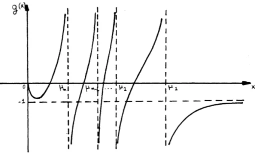
It is interesting for computational purposes to investigate when these m roots are real or complex. We assume first that the m poles of the service time distribution are dinstinct and there are no zeros of f3. (x) which coincide with any pole of f~(-x).
If g(x) f,(x)f, (-z)-1, then lim_0o+ g(x) = _ < and limz g(x) =
-1. Graphically g(z) is presented in figure 5.
Figure 5: g(x) with all m poles of f.(z) real
Therefore all the m roots are real. If there are zeros of f; (z) that coincide with poles of f; (-x) then there may be roots which are complex.
An interesting case is also C,/E,,1. Then g(z) in this case is presented in figure 6.
Figure 6: g(x) with only 1 pole of f,(z) real
If m is odd then there is only one real root (figure 6). If m is even then there are 2 real roots.
As a result, since the algorithmic complexity of the determination of the roots increases if the roots are complex, we can say that the algorithmic complexity increases when the service time distribution becomes more homogeneous (E,, for example, in the sense that the rates of the stages are the same ).
2. EEm/8.
In this case (22) becomes
kA z)k(mm = 1 j(xz)=mJ(1e kA )) j=1 ...
(26)
Substituting (26) to (21) we get
kA di .w (j-1);
smA - m(k,+ t =-ie =
If we define c - =1 ije " (IEVI < 8) then we must solve the equation:
kA k
sm/s - m(kA )+ = z
Then on the boundary C2 of D (figure 7) as Ixl - oo
Im(k+ zk ),EI < S mis < - smilI
Figure 7: Rouche's theorem for Ek/Em,I QS
In particular, for x = 0 and i = (s,O,...,O) the above strict inequality be-comes equality. Thus, in order to have the required strict inequality, so that we can apply Rouche's theorem we consider a small semicircle and use Taylor expansion to take as x O+ with Re{x} > 0
Im#(kA )A,t = IsmP(i -- +o(x))l < lzx - smIl if p < 1
IkA + X)j Am
In the boundary C1 (x = ia) one can verify after straightforward algebraic
manipulations that the above strict inequality holds.
unique root in D, which satisfies (23). Furthermore, since we have proved that there are no roots for Re{z} < 0 and the radius of C2 of the closed domain D
can get arbitrarily large we conclude that if p < 1 there is a unique root for every combination of which satisfies (23). V
3. C,,/M/s.
For m = 1 we find that (22) becomes
f~.(X)f(- ) = 1 z = s(1- f(z))
Then w is the unique real root of the equation
w = f;,(s,(1 - W))
which is the well known result from G/M/s theory. At this point we remark that our result which was obtained for the class of C, interarrival distributions is still valid for a general distribution. This observation comes to support the conjecture in section 3 that our solution is still valid even for the GI/R/s QS.
4. EnIC2/s
This QS, which was studied by Bertsimas and Papaconstantinou (1986), has the very attractive property that all the a(s, 2)- s +1 roots are real and thus
the algorithmic complexity of this QS is low. In fact an O(s3) real arithmetic algorithm was proposed.
2.6 General remarks
1. We now investigate under which conditions we can find an explicit equation for , in the sense that (21) is an implicit equation involving the functions
ej (x) (j = 1, ... , m), which are not in general known explicitly. This property
is algorithmically useful since an explicit equation for can be easily solved by numerical means. We exploit the fundamental result in the theory of
polynomial equations. Since (21) is a polynomial equation for (z) (which has m roots, 1(z), ... , 0(z)), a closed form expression for j(z) can only be
found for m < 4. For m > 5 we cannot in general find an explicit formula. For example for m = 2 the + 1 roots z(wj) (wi = f(z(wj))) satisfy the ·following equation:
(s-2j)A(fT .(X(Wi))-(+-sl+2)+qlsAl,.(x(wi))+2x(wi) = O, j = O,...,s
where
A(Y)- (,2 - 1 + YqCs) 2 + 4A12(1 - ql)y
2. The complexity of the problem increases extremely fast with the number of roots, which increase exponentially in s,m, when both s,m vary. For this reason, it is better to use low values for m (m = 2,3,4) to approximate a service time pdf avoiding the venture of determining exponentially many roots. In the opinion of the author, for all practical purposes the value of
m = 2 is a tradeoff between accuracy and simplicity, which has the additional
advantage of the rather unexpected real arithmetic.
3. In the attempt to investigate Cox's idea of introducing complex transition rates, to obtain complete generality in synthesizing any pdf with rational Laplace transform, we observe that the general proof that there are a(s,m) roots of equation (21) did not depend on the assuption that IL, ...,c , or Al,..., Am are real. Since, in order to have a valid pdf with complex poles we have to have m > 2, the simplest multi-server model involving complex transition rates is Cs/Cs/s which has (,+2)(8+1) = 0(s2) complex roots. 4. A very promising idea lies in the exploitation of an old and very widely used
idea in the field of Electrical Engineering, namely transfer functions. By re-ducing the order of a transfer function (which corresponds in queueing theory
terms to the rational Laplace transform of the pdfs) we can find an excel-lent approximation of a large order pdf by a low order pdf. This decreases tremendously the algorithmic complexity of the problem.
2.7
The algorithm for the unsaturated probabilities
Returning to the assumed form of the probabilities P,, n
>
, = 1...,k,tN
=s we observe that the most general solution must be a(v,m) Pn,,= D, Rj w n> s, = 1,...,k, I = s (27) j=l where from (7) -(1p) = 2,...,rk = = D(w,) + Ar+l
and RIj satisfy (6). For each j (corresponding to the root wj) the coefficients R
satisfy a system of a(s,m) linear homogeneous equations (6). Thus for a fixed j.
we can find the ratios RrO f(i, wj) recursively. Thus the unknowns are the
coefficients Bj Dl,jR(o,...,o,o)3 i.e. there are a(s,m) unknowns. Therefore
a(o.,m) 1-1 (1 - p )= k
P,, = B H
,+
) f (i,w j ) w n>
s,=1
k
lS j=l r=l (w,) + 7 k'
Furthermore, from (25) we observe that the generating function of f((t, wj) is
Gj(f) = U = - 1 1(blr(wj)Zl b+.. + bm1r(Wj)Zm)it (28)
R(o), 1,= b ,(W,)
Up to this point the remaining unknowns are the coefficients Bj and the unsaturated
probabilities P,,:, n < s, I = ,...,k, it = n. There are two strategies for
finding these unknowns. Strategy A
1. Using the equation (2) for n < s we express the unsaturated.probabilities Pn,a,, as linear combinations of the coefficients Bj, i.e. finding recursively from (1),
(2) the coefficients g(n,l,ij) in the expansion:
o( ,m)
P,=
Bjg(n,l,ij)
n<s,l=1,...,k,I
=n (29)$=1
Thus after this step only the coefficients Bj(j = 1,...,a(s,m)) remain un-known.
2. Using the identities Pn-1,k, = 0 n < s, [N = n we find =0( +n 1) = ('+s )
linear homogeneous equations for Bj. Selecting ( + )-1 of them and using the normalization equation
E P,,,~ = 1 (30)
we find a linear non-homogeneous system of a(s, m) equations with the a(s, m) unknowns Bi .
Strategy B
There are (n+m-1
There are kE' (n) = k(s-1) unsaturated probabilities Pn, and ( + )
unknown coefficients Bj. Using equations (1), (2) for n < s we find k(s- 1)
*+rn-1
equations for Pn,,,.. Also, the equations (1) for I = 1 and n = s give another ( i) equations that involve the unknown quantities Pn,1,1 (n < s) and Bj. So, we have a
linear homogeneous system of k(s- 1) + ( ) equations with the same number of unknowns. Using the normalization equation (30) we find a linear non-homogeneous
system, which can be solved by numerical methods.
3
The system-size probability distributions and
the usual performance mearures
In this section we find closed-form expressions for the quantities Pn, P-,, P, P+
(see section 1.2) for n > s. Also closed-form expressions are provided in section 3.2
3.1
System-size probability distributions
Concerning the distribution of N we state the following proposition.
Proposition 3
The general-time probabilities of the number of customers in the system have the following form: if n>s p j=Gli Bj - I u(J) -wj) w,
=(J'm) Bj EL=I EI=n g(n, 1, ,j)
if
(31) n<8where Gj(i) is computed from (28).
Proof
In general
Pn=
Then for n > s, using (27), we take:
k
=1 jE=min(n,*)
o(,,m) k
P = E (Dlj)
(
Rj)
wu"j= = F1=o
But E1I= R;,j = Uj(1) = Gj(R(o ... ,o)j from the definition of the generating
func-tion Uj(z-) and using (28). Also from (7)
k l (1 -p,)Ar
1=1 r=1 z(w,) + Ar+i
= Dj X + (wi)( - Wj)
x~uwj)
where we have used the identity that
k pf) 1-1 Wi = f/ ((j)) = (w) + A, II 1-1 x(Wj) + Al r=1 (1 - p,)A, z(W) + Ar Therefore P a(m) D A1+ z(wj) U (1) (1 w,) j=1 n>s (32)
Using the definition of B = DljR(o,...,o,,)j (31) follows for n > a. For n < s, using (29), (31) follows easily.
Pn,l,i
EDj=
D jConjecture
Although the method of stages we presented is not immediately extendable to dis-tributions, which do not have rational Laplace transform, we believe that this
sep-arability property holds for the more general model G/R/s, but does not hold for
GIG/s where G for the service time pdf does not belong to the class R. The reason
for this difference is that it is the structure of class R and its probabilistic interpre-tation that enable us to "separate" the equations for the roots wi. Summarizing we
conjecture that for the G/Rm/s QS
Pn=
Z
Ljw n > sj=1
where wj are the ( s ) roots of the following system of equations
w=f.() (Iwl<l)
Zijej()=z
such that >i=j=1 j=1
f.(x)f(- Oi(x)) = 1 (i = l,...,m)V
Concerning now the pre-arrival probabilities we prove the following proposition 4
Proposition 4
The pre-arrival probabilities P¾, P, P and the post-departure probabilities Pn+ for
n > s can be expressed as follows:
1 G(*,M) P
=,
= E Bj f(iwj) ( + x (j))n+l n s, i = (33) j=1 1 (4m) P P =1P+
E n2 BjGj(i(A 1 + x(wj))w+ n > (34) j=l ProofIf we define the event AAO =Arrival about to occur in (t, t + t) then we take
z =P
=,=Pr{N = n n R =i n AAO}Pr{(u,=(N = n nR = i n R, = l) n AAO} _
Pr{u =R, = n AAO}
EL
Pr{AAOIN = n n R = R. = }P{ = n n = n = I}-=1 Pr{AAOIRo = })Pr{R = 1) But since
Pr{AAOIN = n n R = n R = l} = Pr{AAOIR. = I} = xAp6t
and Pr{R = } = Eri {Pr Il_ 1 1( - pm)} A . we take =1 AplP,l,;S =1 API XIYtr=l{Pr 1 (1m)} since
E=l
pt Zr,={Pr,
(1
- Pm)}1.
Therefore, using (27) and (35) we have:
1 a(,rm) k P-n= , {Z jplD,} RJ- W j=1 5=1 Also from (7) k ApjDj=1 l=1 k = AlplD1,j 1=1
l-l (1 - p,)A,
r=1 x(W,) + A7+1 = Dj(AXI + x(wj))wjThus from (36), (33) follows. Also Pn = P= 0i=J 1 a(s,m)
=-
Aj=From l=, f(is w;) = Gj (i) and the general relation
Pn-G/G/s QS (34) follows. 7
3.2 System performance measures
1. Mean queue length
If Lq is the length of the queue then
E{Lq} = Z(n - s)Pn
n=
=
P+ which holds for the
= P+ which holds for the
(37) P-, n,s i1 = E A1=1 Pn, 1=1 (35) (36) Bj (X1 + z(wi))w}+1 E f (i, Wj)
We substitute (31) into (37) and find a(0,m)
E{Lq}=
E j=1 BjGj(l)+ x(w) j1 -W X(Wj) 1 -Wi2. Proportion of time all servers are busy, Pb,,v oo0
Pebsv = E
n=.
o(,,m)
P = BGA( + 3(Wj)
3. Probability of non-zero waiting time 00 Pr{T > 0} = n= 1 a(,,m) P = BGj ((A i=1
+( )) W+i
1- W4
Computational and complexity considerations
4.1
The algorithm
In order to extract numerical results from the formulae presented in sections 2, 3 we propose the following algorithm based on strategy A (see section 2.7).
e+m-1
1. Determination of the ( s ) roots wj of the system of equations (21), (22), (23), (8).
2. Determination of the coefficients f(s, wj) from (6).
3. Determination of the Pn,.aT for n < s as linear combinations of Bi .
4. Determination of the ( s ) unknowns Bj as a solution of a linear system with ( - ) equations.
(38)
(39)
(40)
4.2
Complexity considerations
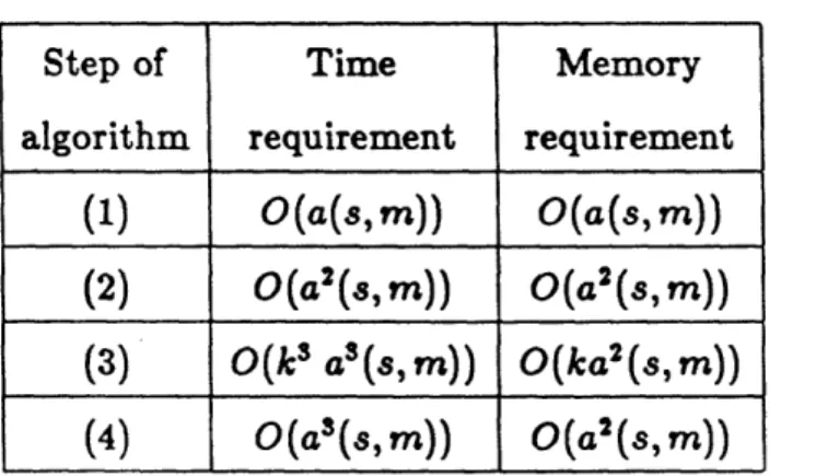
In table I we show the computational complexity of each step of the algorithm with respect to memory and time requirements.
Table I: Computational requirements for the solution of the Ck/Cm/s [
From table I we can make the following observations. Since from a computational point of view the "heaviest" part of the algorithm is the third step, the time com-plexity of this algorithm is of O(ka 3s(s, m)) . We consider the following cases:
1. For a fixed m, the algorithm is polynomial in the number of servers s since
O(kSa3(s,m)) = O(ksS(m-I))
2. For a fixed s, the algorithm is still polynomial in m, since
O(ksa3(s, m)) = O(km 3')
3. When both m, s vary then the algorithm becomes exponential, since
O(k 3a3(s, m)) = O(ke ' + 'm)
As a result, this algorithm has a polynomial time complexity when only one of the parameters m, s vary, but it is exponential when both parameters vary. We can also observe that this algorithm is always polynomial in k. The above results verify that the complexity of the analysis of the Ck/C,/s QS increases much faster with the service time than with the interarrival time pdf. That is, we expect for example that the derivation of numerical results for the M/C,/s QS is much harder than for the C,/M/s QS.
4.3
The numerical solution of the C
2/C
2/sQS
To fully gauge the performance of the proposed algorithm we programmed it in FORTRAN, because of its inherent superiority in accuracy and speed and in BASIC because of its greater availability in microsystems. The first program has been run on a CYBER 171 and the second on a SPECTRUM 48K, in order to prove that even for such a "difficult" model exact numerical results can be obtained by a practitioner on a small personal computer.
The reasons we selected this model are:
1. It is representative of the general behavior of the algorithm for more general models.
2. It is in real arithmetic.
3. Its complexity 0(s3) is not very high.
4. This model allows the determination of exact results when the coefficients of variation of the interarrival and of the service time pdf are both greater than 1.
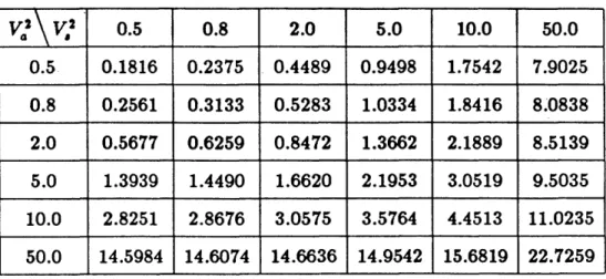
Merely as an illustration of the stability and accuracy of the present algorithm, we present in table II a few typical results for the C2/C 2/15 case with p = 0.9
and the conditions ul = 2, ql = 1- v?, 2 = (l - q), Al = 2A, Pi = 1 -v,
A2 = A1(1 - Pl) (two moment-fit; V,V,2 are the coefficients of variation of the
interarrival and service distributions respectively).
Table II: E{Tq} as a function of V.2, V2 for the C2/C2/15 QS
4.4
The numerical solution of the Ek/C
2/sQS
This QS is solved by Bertsimas and Papaconstantinou (1986). In order to illustrate the dependence and the sensitivity of this algorithm on k we prepared another
program for the analysis of the Et/C2/ QS.
After careful and time-consuming tests of our computer programs we have pro-duced extensive numerical results for a wide range of the parameters 8, p, k, 1, 2
and q which complement or extend (being always in full agreement with ) the re-sults of Kuhn (1976) for the E1,2/M/s, Sakasegawa (1978) for the Ek/E2/s, Ishikawa
(1979) for the M/E 2/s, Hillier and Yu (1981) for the Ek/E 2/ , Hokstad (1982) for
the M/H 2/s, van Hoorn (1983) or Groenevelt, van Hoorn and Tijms (1984) for the
M/H 2/s and M/E,2/s and finally of de Smit (1983b) for the M/H 2/s, E2/H 2/s
and E5/H 2/s systems.
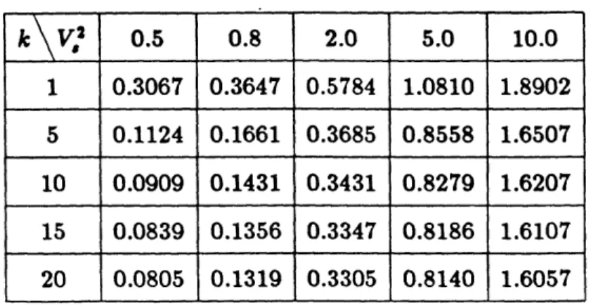
In table III we illustrate the dependence of the mean waiting-time Iz E{T} (in
units of service time) for the model Ek/C2/15 (p = 0.9, Al = 0/2 for V,2 < 1
and q = "I for V,2 > 1). This selection of parameters coincides with that of Groenevelt, van Hoorn and Tijms (1983) but differs from de Smit's (1983b).
Table III: tz E{Tq} for the Ek/C2/15 QS as a function of V,2 = - VJ2|
This typical example demonstrates the well known for the M/G/1 QS deleterious effect of irregularity in service times. We observe that the numerical results as k increases converge quickly to the corresponding limiting (for k - oo) D/C2/s
and thus render any computations for k greater than a certain small value almost unnecessary.
Finally in figure 8 we present the computational times in CPU seconds on a CYBER 171 as functions of k and s.
5
Some concluding remarks
Several discussions of the major computational problems arising in the numerical solution of multi-server queues with non-exponential service time can be found in Yu (1977), in Tijms and van Hoorn (1981) and Neuts (1981).
For high values the fact that
1. the monumental, ten-year computer-oriented project of Hillier and Yu (1981) was hinderd by severe computational feasibility limitations, and
2. the approaches of de Smit (1983b) Groenevelt, van Hoorn and Tijms (1984) lead to rather extreme levels of computational complexity,
seem to indicate that the key to success in making an intrinsically difficult QS solvable lies in the selection of a suitable solution strategy, like the one presented in this paper.
Strongly critical remarks have been made in the past both on the merits of queueing theory (see e.g. Neuts (1981), p.42 or van Hoorn (1983), p.101) and on unwarranted algorithmic claims in the applied literature on stochastic models. Being fully aware of the need for the probabilist to be very closely involved with the algorithmic analysis of a problem, we have undertaken ourselves the painful" task of programming and testing our algorithms.
5.1 Open problems
In this paper we extended the method of stages to its complete generality solving the general class of multi-server Markovian queues. In our opinion, the major problems that are of importance in the field of theoretical and applied queueing theory are the following:
1. Find the waiting-time distribution under different queue disciplines, e.g. LCFS (Last Come First Served), SIRO (Service In Random Order). This problem
seems extremely hard, since very limited results are known. Even for MIMIs the expressions for the pdf of the waiting-time of an arriving customer are of extraordinary complexity.
2. Find the steady-state probability distribution for the class of non-Markovian multi-server queues, thus settling the conjecture in section 3.1.
3. Perform busy-period analysis. 4. Perform transient analysis.
Concerning possible extensions of the present approach we believe that the following problems are tractable:
1. Extend this theory to solutions of multi-server QS where priorites are allowed. 2. Generalize this theory to the domain of transient behavior of queueing
sys-tems.
3. In the field of computational queueing theory develop a general purpose algo-rithm to approximate a general distribution not generally in the class R with one that belongs in this class preferably of low order. Then by exploiting the results of this paper we will have an approximate solution of the G/G/s QS . 4. Introduce complex transition rates to obtain complete generality in
synthe-sizing any pdf with rational Laplace transform.
We end this paper by expressing the hope that the solution strategy we presented might be the Ariadne's thread to a general but tractable calculus of rational distri-butions for multi-server queues.
Referrences
ALLEN, B., ANDERSSEN, R.S. and SENETA, E. 1977 "Computation of stationary measures for infinite Markov chains", in NEUTS, M.F. (Ed) Algorithmic methods in probability", TIMS Studies in the Management Sciences, 7, North Holland. BERTSIMAS,D. 1986, "An analytic approach to a general class of G/G/s queueing systems", Master Thesis, Massachussetts Institute of Technology.
BERTSIMAS,D. and PAPACONSTANTINOU, X. 1986, "On the steady-state so-lution of the Ek/C2/s queueing system", Europ. Jour. Oper. Res., accepted for
publication.
COHEN,J.W. 1982, "The single server queue", North Holland.
COX,D.R. 1955, "A use of complex probabilities in the theory of stochastic pro-cesses", Proceedings of the Cambridge Philosophical Society, 51, 313-319.
GROENEVELT, H., Van HOORN,M.H. and TIJMS, H.C. 1984, "Tables for M/G/c queueing system with phase-type service", Europ. Jour. Oper. Res., 16, 257-269. HILLIER,F.S. and LO,F.D. 1971, "Tables for multiple-server queueing systems in-volving Erlang distributions", Technical report No 31, Dept. of Operations Re-search, Stanford University.
HILLIER,F.S. and YU,O.S. 1981, "Queueing tables and graphsr", Publications in OR series (ORSA), Vol. 3, North Holland, New York.
HOKSTAD,P. 1978, "Approximations for the M/G/rn queue", Oper. Res., 26, 511-523.
HOKSTAD,P. 1979, "On the steady-state solution of the M/G/2 queue", Adv. in Appl. Prob., 11, 240-255.
HOKSTAD,P. 1980 "The steady-state solution of the M/K 2/rn queue", Adv. in
Appl. Prob., 12, 799-823.
HOKSTAD,P. 1982, "Some numerical results and approximations for the many server queue with non-exponential service time", Dept. of Mathematics, University
of Trondheim.
HOKSTAD,P. 1986, Bounds for the mean queue length of the M/C 2/m queue",
Europ. Jour. Oper. Res. , 23, 108-117.
van HOORN,M.H. 1983, Algorithms and approximations for queueing systems", Mathematisch Centrum, Amsterdam.
ISHIKAWA,A. 1979, "On the equilibrium solution for the queueing system GI/Ek/m", TRU Mathematics, 15, 47-66.
KLEINROCK,L. 1975, "Queueing systems; Vol. 1:Theory", John Wiley and Sons, New York.
KUHN,P. 1976, Tables on delay systems", Institute of Switching and Data Tech-nics, University of Stuttgart.
NEUTS,M.F. 1981, Matrix geometric solutions in stochastic models :an algorith-mic approach" ,The John Hopkins University Press.
NEUTS,M.F. 1984, "Matrix-analytic methods in queueing theory", Europ. Jour. Oper. Res., 15, 2-12.
OVUWORIE, G.C. 1980, "Multi-channel queues: a survey and bibleography", In-ternational Statistical Review, 48, 49-71.
POLLACZEK,F. 1961, Theorie analytique des problemes stochastiques relatifs un groupe de lignes tlephoniques avec dispositif d' attente", Gauthier, Paris. SAKASEGAWA, H. 1978, "Numerical tables of the queueing systems 1:Ek/E 2/s",
Computer Scince Monographs No 10, The Institute of Statistical Mathematics. SEELEN,L.P. 1986, "An algorithm for PH/PH/c", Europ. Jour. Oper. Res., 23,
118-127.
de SMIT,J.H.A. 1973a, Some general results for many server queues", Adv. in Appl. Prob., 5, 153-169.
de SMIT,J.H.A. 1973b, On the many server queue with exponential service times', Adv. in Appl. Prob., 5, 170-182.