Analysis/development of a crash sensing algorithm using multiple accelerometers

(1)

Analysis/Development of a Crash Sensing Algorithm Using Multiple Accelerometers

by Fon-Jui Tsai

Submitted to the Department of Electrical Engineering and Computer Science in Partial Fulfillment of the Requirements for the Degrees of

Bachelor of Science in Electrical Engineering and Computer Science and Master of Engineering in Electrical Engineering and Computer Science

at the Massachusetts Institute of Technology

May 23, 1997

and to grant others the right to do so.

Denartment.of Eleatrical Fns•ineeriny and Computer Science 7

artin Schmidt ,, iervisor

Authur C. Smith Chairman, Department Committee on Graduate Theses

r

T

2

1997

Author Certified by Accepted by. P -°

a

(2)

Analysis/Development of a Crash Sensing Algorithm Using Multiple Accelerometers

by Fon-Jui Tsai

Submitted to the

Department of Electrical Engineering and Computer Science

May 23, 1997

in Partial Fulfillment of the Requirements for the Degrees of Bachelor of Science in Electrical Engineering and Computer Science and Master of Engineering in Electrical Engineering and Computer Science

ABSTRACT

Single-point, multi-directional crash sensing is a relatively new concept in collision detection, and there re-main many question which today's research and study have not been able to answer. The objective of the thesis is to analyze and understand the benefits of using multiple accelerometers placed in multiple directions and, furthermore, to measure the effectiveness and the applicability of the multi-axes crash sensing algorithm. The results indicate that the ability to detect high speed angle collisions is greatly enhanced when lateral and vertical signals are used. The study also finds that the additional information provided by lateral and vertical signals only slightly enhance the ability to detect severe pole collisions. In addition, the lateral and the ver-tical information alone cannot successfully categorize the collisions; the longitudinal signals must be used to filter the rough road and other long-duration events.

Thesis Supervisor: Martin Schmidt

(3)

6.2.1. 6.2.2. 6.3. 6.3.1. 6.3.1.1. 6.3.1.2. 6.3.1.2.1. 6.3.1.2.2. 6.3.1.2.2.1. 6.3.1.2.2.2. 6.3.1.2.3. 6.3.1.2.4. 6.3.1.2.4.1. 6.3.1.2.4.2. 6.3.1.2.4.2.1. 6.3.1.2.4.2.2. 6.3.1.3. 6.3.1.3.1. 6.3.1.3.2. 6.3.2. 6.3.2.1. 6.3.2.2. 7. RESULTS 7.1. 7.2. 7.2.1. 7.2.1.1. 7.2.1.2. 7.2.2. 7.3. Patents Analysis

Independent Threshold Method Threshold Requirements Longitudinal Requirements Lateral Requirements Acceleration

Velocity

Causes of the Dip

Algorithmic Enhancements Using the "Dip" Consistency of the Velocity

Rectified Energy Lateral Rectified Energy Combined Rectified Energy Arbitrary Decay

Combined Rectified Energy Calculation Vertical Requirements

Vertical Velocity

Vertical Rectified Energy Structure of the Algorithm Angle Collision Detection Pole Collision Detection

Initial Results

Complete Crash Detection Statistics Timeliness of the Deployment

Angle Collisions -Single-Axis Algorithm vs. Multi-Axes Algorithm Pole Collisions -Single-Axis Algorithm vs. Multi-Axes Algorithm Robustness of the Algorithm

-Angle Collisions -Single-Axis Algorithm vs. Multi-Axes Algorithm Rough Road Discrimination

8. CONCLUSION

APPENDIX A. Longitudinal, Lateral, and Vertical Velocity Signals of Typical Frontal, Angle, and Pole Collisions

APPENDIX B. Threshold Determination: Angle Collision Detection Pole Collision Detection APPENDIX C. Performance: Timeliness

Robustness REFERENCES ADDITONAL READINGS ACKNOWLEDGMENT 90 100 112 122 123 133 134

(5)

Chapter 1 1. ABSTRACT

Single-point. multi-directional crash sensing is a relatively new concept in collision detection, and there remain many question which today's research and study have not been able to answer. The objective of the thesis is to analyze and understand the benefits of using multiple accelerometers placed in multiple directions and, furthermore, to measure the effectiveness and the applicability of the multi-axes crash sensing algorithm. The results indicate that the ability to detect high speed angle collisions is greatly enhanced when lateral and vertical signals are used. The study also finds that the additional information provided by lateral and vertical signals only slightly enhance the ability to detect severe pole collisions. In addition, the lateral and the vertical information alone cannot successfully categorize the collisions; the longitudinal signals must be used to filter the rough road and other long-duration events.

(6)

Chapter 2 2. OBJECTIVE

Currently in the SIR (Supplementary Inflatable Restraint, i.e. the airbag) algorithm, the severity of the crash and the deployment of the airbag are determined by calculations and analysis of a single accelerometer aligned in the front-rear directions (referred to as the longitudinal direction hereafter). However, some European and Japanese car makers are experimenting and, in some cases, already using multiple accelerometer inputs to determine the severity of the crash. The objective of this project is to investigate the benefits of using multiple accelerometers in the crash sensing, and furthermore, develop a feasible implementation and algorithm which utilize multiple accelerometer inputs. This project is to focus on cases in which several accelerometers are packed closely in space such that they can be approximated to originate from a single point. However, the orientation of these accelerometers

corresponds to the longitudinal, the lateral, the vertical, or other arbitrary axis relative to the vehicle. The scope of the thesis includes analyzing raw crash data, creating a functional algorithm, generating a algorithm model which is tested through extensive simulation.

(7)

Chapter 3

3. BACKGROUND

3.1. Industry Standards in Airbag Technology

Supplementary Inflatable Restraint (SIR) systems, or airbags, are becoming standard equipment on most cars and light trucks sold today. In the past, the predominant crash sensing system was a multi-point sensing system in which the deployment decision is based on crash sensors placed at strategic locations in the vehicle. However, the industry trend has since been toward a single-point crash sensing system'.

(8)

The inflatable restraint system design considerations can be divided into three areas: vehicle system, electronic diagnostic module, and crash sensors.

3.1.1. System

In a deployment event, the inflatable restraint system functions in less than 100 milliseconds2. The effectiveness of the system is determined by the rate and the state of the deployment at given time during the crash event. The inflatable restraint system which includes the inflator and bag assembly, diagnostic module, crash and safing sensors, is designed to perform with respect to other subsystems of the vehicle, such as the vehicle structure, steering control system, instrument panel, seat belts, and the seats. The inter-relationship between these subsystems must be considered in order to optimally protect the occupant in a collision3.

3.1.2. Electronic Diagnostic Module

The diagnostics module and sensors play a critical role in the overall effectiveness of the SIR. The module must be well designed in the sensing technology to ensure the accuracy of the deployment, as well as in robustness in order to sustain long life under severe environmental conditions. In addition, to ensure the safety critical nature of the system, a diagnostic module is used to continuously monitor the firing circuits and provides driver warning. Furthermore, a redundant energy source is crucial since the battery may be cut off in a severe collision4.

3.1.3. Sensors

The system considerations in the design of a crash sensor include the number of sensors needed and the operational logic in the sensing system. In addition, the locations and the directions of these sensors are significant Essentially. the goal of an ideal sensing design and algorithm is to maximize the ability to differentiate deploy crash events from the non-deploy crash events while still providing timely

(9)

deployment. In addition, the sensor design must be flexible to allow transferring from one vehicle platform to another5. It is the sensing considerations which are explored in this thesis.

3.2. Efforts in Using Multiple Accelerometers

In most of the vehicles equipped with the airbags today, the crash sensing algorithm uses only the longitudinal signals to determine the severity of the crashes6. Although some car makers are

experimenting with using multiple accelerometers in multiple directions, the concepts are still relatively new.

Toyota Motors of Japan has patented the concept of using the longitudinal and the lateral acceleration vectors to determine the angle of the collision. The actuation of the airbag is determined by comparing the magnitude of the crash signals to a set of predetermined thresholds based on the calculated angle of impact. Because the angle of impact cannot be accurately determined, the calculation categorizes the angle into one of the 10 groups: ±150, ±30', ±45', _{+600, and}_±750. _{The thresholds used for}

comparison are stored in a large look-up table .

Daewoo Electronics extended the above idea to incorporate the vertical signal in the crash sensing algorithm. Specifically, the algorithm proposed by Daewoo is aimed at discriminating between oblique (angle), frontal barrier, and center pole collision. The deployment decision is based on the thresholds placed on the velocity signals in all three directions. Daewoo claims that the angle collisions can be easily detected with the lateral velocity signal. Furthermore, the vertical velocity can be used to effectively detect the pole collisions8.

Lastly, algorithm engineers from Schrobenhausen, Germany also believed in a crash sensing by determining the angle of the impact. In a patent filed jointly by several engineers, the proposed method of determining the angle is to use dual accelerometers placed at ±0 from the longitudinal axis or the

direction of travel. By resolving these two vectors using cosine law, the angle of the collision can be better determined. The magnitude of the resolved vector is compared to the variable threshold which is based on the calculated angle9.

(10)

While these patents outline the crash sensing concepts, very little detail is disclosed. Part of the objective of this thesis is to duplicate the experimentation and the results described in these patents.

3.3. Current Single-Axis Crash Sensing Algorithm

The analysis of the single-axis crash sensing algorithm is based on a current production version developed by a large automotive electronics firm. The algorithm arrives at the deployment decision based on calculations and analysis of the vehicle's longitudinal acceleration, velocity, and displacement. Prior to discussing the algorithm with multiple accelerometer inputs, it is essential to explore and understand the functionality of the basic single-axis algorithm which uses only the longitudinal accelerometer input.

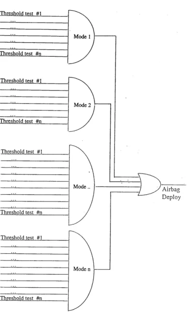
The deployment logic of the current production algorithm is based on the idea of classifying the severity of the crashes into different categories. Each of these categories represents a crash scenario in which the airbag must deploy. For example, a category, or a "mode" as they are sometimes referred to, may be used to catch the high severity events on time and act as back-up mode of deployment for less severe deployment events. Moreover, other modes can be set to discriminate threshold, angle, and offset barrier events. Lastly, another mode can be designed to detect events that are of longer duration, and the examples include poles, some angle, and lower speed threshold frontal events.

The basis of the algorithm details how the collisions are classified into separate categories. Specifically, the collisions are classified based on the behavior of the longitudinal acceleration. There are different traits associated with the acceleration signals of different types of crashes, and these traits are best identified using the threshold tests. A threshold test is exactly what the name suggests: a certain flag is set when the signal exceeds a preset level. Of course, the behavior of the acceleration signal is not the only criteria tested. The velocity (integration the acceleration) and the displacement (integration of the velocity) are two other measures which can provide valuable information. Consequently, many threshold tests are used to evaluate and classify the collisions, and in most cases, a collection of threshold tests have

(11)

to pass in order for the algorithm to conclude if the severity of the collision requires the deployment of the airbag.

Until now, the word "threshold" has been used loosely to mean a preset level which, when it is crossed, can correctly categorize the severity of the crashes. These thresholds are either based on or derived from the acceleration, the velocity, and the displacement of the vehicle in a crash. First of all, the fundamental thresholds are the acceleration, the velocity, and the displacement, which are compared against the acceleration, the velocity, and the displacement of the vehicle. Next set of thresholds examines the behaviors of the acceleration, the velocity, and the displacement. Lastly, some thresholds are time-dependent. Specifically, these threshold tests require that the signal crosses a preset level for a finite period of time. These time-dependent threshold tests can be used to separate cases which the signal has crossed the thresholds briefly due to noise or other factors and fall below the thresholds immediately after. In conclusion, the categories, or the modes, of collisions are no more than a combination of different threshold tests. When a set of threshold tests is exceeded, the collision can then be categorized into respective modes.

The deploy logic of the current crash-detection algorithm can be summarized in the following logic diagram.

(12)

Deployment Logic of the Current Production Algorithm

Figure 1: Deploy Logic of the Single-Axis Algorithm

A possible limitation of the current production algorithm is that only the longitudinal signals are

used in the decision making process. This may be adequate for the moment, but some European and Japanese car makers are beginning to experiment with the idea of incorporating accelerometer inputs in both the lateral and the vertical axis into the crash sensing algorithm. Furthermore, Daewoo Electronics

(13)

Co. has recently patented the idea that it is possible to accurately categorize the different types of crashes using tri-axial accelerometer inputso0. Realizing the potential in this methodology, this thesis is to investigate the benefits and the shortcomings of using multiple-axis acceleration inputs in crash sensing.

(14)

Chapter 4 4. SCOPE

The idea of the single-point, multiple-axis crash sensing algorithm is certainly not unheard of in the airbag industry. Research has been done in this area by almost all the major leaders in the automobile industry, and in fact, there are several existing patents focusing on this methodology". As a whole, however, the development of the single-point, multiple-accelerometer algorithm is still relatively new, and there remains room for expansion. The following lists some of the algorithms which have previously been considered but not fully explored. Furthermore, the following also includes the new approaches to the algorithm which are examined in detail. The study of these algorithms and the results discovered constitutes the main bulk of the thesis.

(15)

4.1. Independent Threshold Method Contrasted with Correlation Method

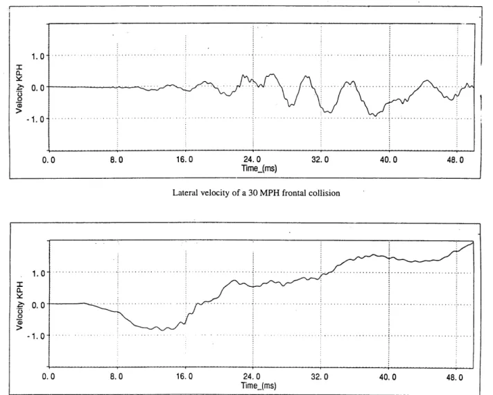
The first step of the algorithm analysis is to examine the lateral signals, and in the course of study, try to establish the correlation between the longitudinal and the lateral signals. From the previous studies and experiences, the current production algorithm exploits the information contained in the longitudinal signals. Using this knowledge as the foundation, the lateral signals can be used to facilitate the current algorithm by strengthening the areas which are weak in the current algorithm. A specific area may be the angle collisions. Because the vehicle makes contact with the barrier at an offset angle, the longitudinal acceleration of the vehicle is weaker. However, the lateral signal may be able to provide additional information. Following is a comparison of the lateral velocity between a 30-mph frontal collision and a 30-mph angle collision (the car collides with the barrier at a 300 angle).

(16)

0.0

.---1.0

0.0 8.0 16.0 24.0 32.0 40.0 48.0

Time_(ms)

Lateral velocity of a 30 MPH frontal collision

Lateral velocity of a 30 MPH angle collision (barrier offset at 30 degrees)

Figure 2: Lateral Velocity -30-mph Frontal Collision vs. 30-mph Angle Collision

The initial glance suggests that these signals are discernible, but there are several aspects which must be studied in depth. First of all, are the above signals representative of all the other crashes of the similar type? Second, is the "dip" in the velocity as shown in the bottom graph a characteristic of all the 30 MPH angle collisions, and what does this dip represent? Furthermore, do the magnitudes of the lateral signals remain essentially unchanged across vehicle platforms? Last and the most important of all, is there a correlation between the longitudinal and the lateral signals? The answers to these questions can essentially lead to two possible algorithms. First, if the longitudinal and the lateral signals are not correlated, the two signals can be examined separately to arrive at the deployment decision. Specifically, two sets of thresholds are used for the longitudinal and the lateral signals, and the airbag is deployed

(17)

when both sets of thresholds are exceeded. However, if there is indeed a correlation between the longitudinal and the lateral signals, an algorithm can derive the deployment decision by manipulating both the longitudinal and the lateral signals. One such approach is to use the magnitude of one signal to adjust the thresholds and the decision making process of the other signal12. For example, let us assume that the longitudinal and the lateral signals are found to be inversely proportional to each other, an

increase in the lateral signal allows the longitudinal thresholds to be lowered proportionally. These two algorithms are the ideal starting points because they will establish the foundation of the multiple accelerometer, multiple-axis sensing algorithm.

The second algorithm described above provides some interesting issues to explore. If there is indeed a correlation between the longitudinal and the lateral signals, can the angle of the collision be accurately determined? If the angle of the collision cannot be accurately determined, can this angle be roughly estimated? Lastly. if the angle can be determined, either accurately derived or roughly estimated, how can this information be used most effectively?

ier

ie

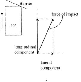
longitudinal component impact 1 = 20 y = 30 lateral component

Figure 3: Forces of an Angle Collision Figure 4: Categories of the Impact Angle

Figure 3 above suggests that if the impact of the collision is at an offset angle, this impact force can be resolved into the longitudinal and the lateral components. Naturally, this is a rough estimate of the

(18)

forces involved in an actual collision. For example, this force diagram assumes that the shear force between the vehicle and the barrier is small and thus can be ignored. Assuming this rough

characterization is accurate, is it possible that the angle of collision can be resolved by geometrically manipulating the longitudinal and the lateral signals. If so, how accurately can the angle be determined? Furthermore, if the angle can only be estimated, is it possible to categorize the ranges of the angle such as shown in figure 4?

While the lateral signals may provide useful information in the cases of angle collisions, the vertical signals may also provide fresh insights. In a recently published patent, Daewoo claims that the vertical signals can be used to detect a pole collision'3. Therefore, part of this thesis is to be devoted to determining if the vertical signals can be used to enhance the algorithm. However, if the algorithm does incorporate the vertical signals, the robustness of the algorithm must be thoroughly tested against the rough road testst

4.2. Rotated-Axis Method

Thus far, the algorithms assume that the orientations of the accelerometers corresponds to the tri-axial orientations of the vehicle. The next step is to explore the possibility of placing the accelerometers at arbitrary orientations. Following is one such example.

t Rough road tests are standard tests which the vehicle with limited or no shocks is subjected to treacherous off-road conditions, and these conditions include the potholes, chatterbumps, railroad crossing, and the vertical drops.

(19)

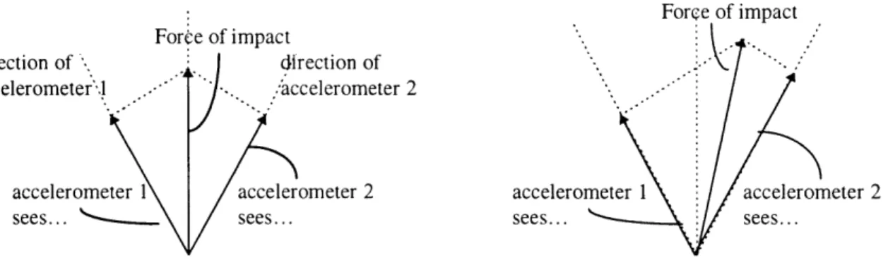
Force of impact oitertid n of :.: direction of accelerometer'. accelerometer •• sees... ..,accelerometer 2 accelerometer 2 sees...

Figure 5: Offset Accelerometers -Long. Force Figure 6: Offset Accelerometers -Offset Force

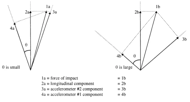
In the above case, two accelerometers are placed at the same offset angle from the longitudinal axis. If the force of impact is along the longitudinal axis of the vehicle, both accelerometers must have the same reading (figure 5). This may seem redundant and wasteful at first, but if the force of impact is at an offset angle relative to the longitudinal axis, the reading of one accelerometer is greater than the other. The analysis is carried out using the data from the accelerometer with higher readings. The advantage of this algorithm is that it has the potential to represent the magnitude of the crash signal more accurately than if the accelerometer is placed along the longitudinal axis (figure 7). Due to the noisy nature of the acceleration signal, the overall effects of the noise can be lessened if the magnitude of the signal is the greatest. However, this is only true when the arbitrary angle corresponds closely to the angle of impact. As in the case portrayed in figure 8. the acceleration signals from the offset accelerometers are actually worse representations of the actual crash signals. In addition to examining the signals from these two accelerometers separately, there may be methods which these signals can be resolved to provide more information.

(20)

la. 3a 4b' 0 is l a = force of impact 2a = longitudinal component 3a = accelerometer #2 component 4a = accelerometer #1 component

Figure 7: Offset Forces Evaluated by Offset Accelerometers -0 is small

Figure 8: Offset Force Evaluated by Offset Accelerometers -0 is large

4 sis 0 is sr 3b = lb = 2b = 3b = 4b

(21)

Chapter

5 5. PROCEDURE

5.1. Examine the Raw Crash Data

5.1.1. Primary characteristics

The primary characteristics are criteria used to assess the severity of the collisions. These are the essential characterizations in the decision process of the deployment of the airbag.

(22)

5.1.1.1. Acceleration

Acceleration is the primary crash signal since all others measures (velocity, displacement, etc.) are derived from it. The acceleration signals are collected by placing three accelerometers in longitudinal, lateral, and vertical directions near where the crash sensing module is located, and the focus of the analysis is on the lateral and the vertical accelerations. Using electronic sensors, the acceleration is sampled and digitized at high enough frequency to not affect the analysis.

There are several criteria one can use to analyze the acceleration signal. First of all, the slope of the acceleration can be used to detect unusually large changes in the acceleration signal. The jerk, or the delta acceleration, is calculated by taking the acceleration from the current time and subtract from it the previous acceleration value. However, the instantaneous jerk may not have much practical value because of the oscillatory nature of the acceleration signal. The alternative is to calculate jerk by taking the difference in the acceleration of two points which are separated by some time. The technique used to filter the jerk signal is discussed in the later section.

In addition, the magnitude of the acceleration can be used to classify the severity of the crash. By establishing a minimum acceleration threshold, the severity is based on whether the acceleration exceeds a certain G threshold.

Lastly, the oscillation of the acceleration signal may provide valuable information. In a severe collision, the acceleration signal shows a significant oscillatory motion or characteristics. While some of the oscillation is filtered out through the initial low-pass filtering, it remains an important criteria which must not be ignored.

5.1.1.2. Velocity

Velocity is derived by integrating the acceleration signal. The velocity is the integration of the raw acceleration signal and not the filtered acceleration signal which was calculated and used only for analysis purpose.

The criteria used to analyze velocity is similar to those used to analyze the acceleration. First of all, the magnitude of the velocity is a useful criteria to determine the severity of the collision. It is

(23)

important to note that the velocity threshold must be absolute because, in some cases, the velocity can either be positive or negative. For example, in an angle collision, the vehicle is just as likely to crash into a barrier from the left side as from the right side, and therefore the magnitude of the lateral velocity tends to either positive or negative to reflect the direction of the impact. In addition, there may be

characteristics which are most pronounced in the velocity domain. The lateral velocities of the high-speed full frontal collision and that of the high-speed angle collision are very good examples. The lateral acceleration of a high-speed full frontal collision has a tendency to be oscillatory with the magnitude of the filtered signal varying from -10 G to +10 G. On the contrary, the lateral acceleration of the high-speed angle collision is less oscillatory with the magnitude varying from -5 G to +5 G. However, once the acceleration signals are integrated, a very clear distinction can be drawn. The high-speed frontal collision shows a lateral velocity which is much weaker and oscillates along the x-axis. The high-speed angle collision, however, has a strong lateral velocity which reflects the direction of the impact. This is a characteristic not visible in the acceleration signals of the collisions.

5.1.1.3. Displacement

The displacement is obtained by integrating the velocity signal. Because the displacement is the double integration of the original acceleration signal, some sharper features may be lost in the signals. Therefore, the overall significance of the displacement signal may be limited. In general, the

displacement signals are smoother and reacts to disturbances (sharp drops or increases and peaks in the acceleration signal) slowly. Therefore, the displacement is usually used to analyze the overall magnitude of the collisions and not for distinct pattern recognition and comparison. Furthermore, studies have

shown that in a high severity collision, the relative displacement of the vehicle is a good approximation of the motion of the driver's body under the free-body assumptions' .

5.1.1.4. Averaged Slope

The slope of a signal is a good indication of how the signal is changing over time. It may seem unnecessary to calculate the slope since the slope of the velocity is the acceleration, and the slope of the

(24)

displacement is the velocity, two criteria which have been discussed and examined. One reason is that the slope of the acceleration, also known as jerk, must be explicitly calculated. Since the acceleration is the original raw signal, how it changes over time can provide very useful information. However, the

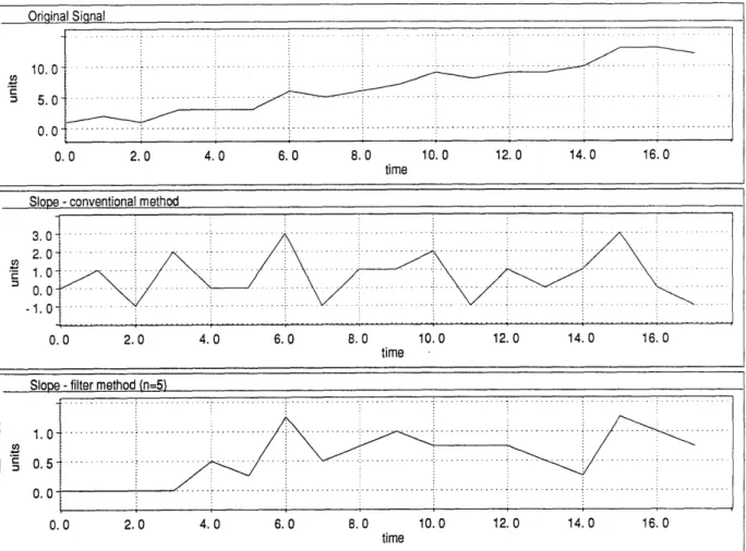
instantaneous slope signal is very noisy and oscillatory (figure 9).

Because the instantaneous slope is noisy, filtering techniques can be applied. One such technique is to generate the slope signal by convolving the instantaneous slope signal with a "box car". In other words, the current slope value is the average of the previous n samples. As n increases, the signal becomes smoother. However, at the same time, some degree of precision is lost as n increases. In addition, instead of finding the instantaneous slope values and perform the average, a more efficient approach is to calculate the slope value by finding the difference between the current value of the signal and that which is n samples back. However, this operation requires memory space of size n. Following is an example which includes the original signal of data, the instantaneous slope, and the filtered slope where n is equal to five.

(25)

Original Siqnal

10.0

5 .0 .. ...

0.0 2. 0 4. 0 6.0 8.0 10.0 12.0 14. 0 16. 0

time

Slope -conventional method

3.0 -2. O 1.0 -0 ... .. .. .... .... ... . ... . . . .... - . 0.0 2.0 4. 0 6. 0 8. 0 10. 0 12. 0 14. 0 16.0 time

Slope- filter method n=5)

0. O

0.0 2.0 4.0 6.0 8.0 10.0 12.0 14.0 16.0

time

Figure 9: Methods of Calculating Slope

5.1.1.5. Energy Indicator

Energy is a more complicated criteria for two reasons: it encompasses a wide scope, and the optimal method to calculate the energy is difficult to determine. The conventional definition of the amount of energy of a moving object is

KineticEnergy = my

(26)

The definition claims that the kinetic energy of a moving vehicle is proportional to the square of the velocity of the vehicle. As the speed increases, the kinetic energy grows with respect to v2. This may not be the most ideal definition of energy because it depends heavily on the measure of velocity. Since the magnitude of the velocity signal is small in the initial stage of the crash, this velocity-dependent energy measurement may not be an ideal discriminating criteria.

Another energy indicator is the rectified energy. The rectified energy is defined below.

Re ctifiedEnergy = f jOriginalSignall

The rectified energy is derived by integrating the rectified signal which is the absolute value of the original signal. Specifically, the rectified energy can be represented by the integrated rectified acceleration and the integrated rectified velocity. These measures are defined below.

Integrated Re ctifiedAcceleration = fOriginalAccelerationl Integrated Re ctifiedVelocitry = f OriginalVelocitn"

The integrated rectified acceleration is the integration of the absolute acceleration signal and the integrated rectified velocity is the integration of the absolute velocity signal. These measures are useful

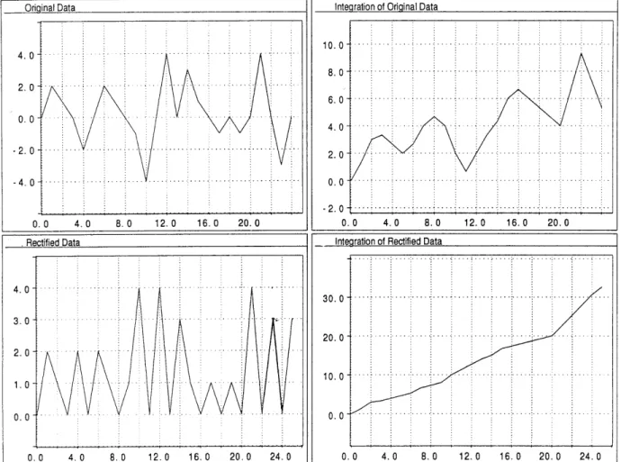
when the acceleration signal tends to zero over a long period of time. For example, when the movement of the vehicle, regardless of the direction, consists mostly of the "back-and-forth" motion, the velocity and displacement tends to zero over time. Consequently, the kinetic energy dissipated is low in the initial stage of the crash. However, the strength of this "back-and-forth" motion may be a key in determining the severity of the collision. This consideration can not be clearly represented using the original definition of the kinetic energy. However, by using the new approach and first rectifying the acceleration or the velocity signal, portions of the original signal. which by normal integration would have been canceled. can now enforce each other. This is shown more clearly in the figure below (figure 10).

(27)

I Oriolnal Data lnteqration of Od~inal Data 0. 0 4. 0 8. 0 12.0 16.0 20.0 10.0-8. 0 6. 0-4. 0 2. 0 0. 0 -2. 0 0. 0 4.0 8. 0 12. 0 16. 0 20.0 Inteoration of Rectified Data

30.

20.

10.

0-0.

0-0.0 4.0 8.0 12.0 16.0 20.0 24.0

Figure 10: Rectified Energy Calculation - Justification for Using the Rectified Signal

4. 0 2. 0 0. 0 -2. 0 -4. 0 .Rectified Data 0.0 4.0 8.0 12.0 16.0 20.0 24. 0

Integration of Original Data

i... i...:... ... ... :...i... ..

.... .. .. ... ...

~

... . ... .. .. .. ....

Orioinal Data I

(28)

In addition to examining the rectified energy measure in longitudinal, lateral, and vertical directions separately, another criteria is to combine the rectified energy measures from some or all directions. Further-more, there are several ways to combine the rectified energy measures from different directions. For exam-ple, it may be useful to combine the three rectified energy components using a variable ratio. The ratio

depends on the relationship between the different rectified energy components.

5.1.2. Secondary characteristics

Secondary characteristics are criteria used to monitor the progress of the collision. While the pri-mary characteristics are used to measure the severity of the collision and to classify the types of collisions, the secondary characteristics are used to monitor the progression of the collision. These are characteristics used to determine if the collision exists and, if the collision is detected, evaluate and monitor the progression of the collision.

(29)

5.1.2.1. Algorithm Enable

Algorithm Enable is a frequently overlooked criteria. With the enable signal, the algorithm knows when the collision has begun. It is a challenging criterion to satisfy because of the implications. For example, if the enabling thresholds are set low, the algorithm is more likely to detect the start of a collision. However, the algorithm may be enabled by typical rough road events, mild disturbances (i.e. external forces applied on the vehicle such as the door slamming), or the inherent noise in the signal. In contrast, if the thresholds are set high, it serves as a natural filter to the non-deployment events. At the same time, the probability is higher that the start of the collision is not detected on time, or it may not be detected at all.

Detecting the start of the collision is important for thresholds which are time-dependent. Although it is undesirable to use time-dependent variables because of the complications and the possible lack of repeatability, it is unavoidable in some cases. In determining the severity of the collision, there are criteria which are effective during a certain time interval after the collision has started. This may be because the thresholds hold true only during a certain period of time after the collision has begun. Furthermore, assuming that decay is not introduced into the signal, most upward-sloping signals will cross a fixed threshold when given enough time. Therefore, the accuracy of when the thresholds start and

stop is crucial. Finally, there may be cases where the initial period immediately after impact contains useful information. In such cases, detecting the start of the collision accurately is critical.

The enable signal can be asserted by using the acceleration signal. If the acceleration exceeds a certain level, the algorithm is to be enabled. The question is in which direction should the acceleration be used to assess and enable the algorithm? In the original algorithm, only the longitudinal acceleration

signal is available for evaluation. Given the lateral and the vertical acceleration signals, can they be used to help assess when the collision has begun? In addition to the acceleration, are there other available criteria which can help better determine the start of a collision? The answers to these questions defines the algorithm.

(30)

5.1.2.2. Collision Progression

Once the collision has been detected, one of the following two scenarios will happen: the

triggering conditions of the airbag are met and the airbag is deployed, or the triggering conditions are not met and the algorithm resets to the initial state. Therefore, there must be a criteria used to monitor if the

collision is still in progress.

This collision progression marker can be set using several criteria. First of all, a minimum acceleration threshold can be used to monitor the severity of the crash signal. If the acceleration falls below a threshold consistently, it is implied that the collision is either a non-deploy event or that the algorithm was enabled unnecessarily. Instead of only keeping track of the present acceleration level, there is a danger in resetting the algorithm when the acceleration signal has a region of very low acceleration. Therefore, the history of the signal may also play a role in the collision progression marker.

Another possible scenario which makes the collision progression marker a crucial factor is in the detection of the collisions which are near the threshold level. In most of these collisions, the collision progression marker must prevent the algorithm from resetting due to the low acceleration input. If the reset does take place, the more severe section of the later acceleration signal may likely enable the algorithm again. By this time, the time dependent threshold can no longer accurately determine the start of the collision and the thresholds are no longer applicable. This problem is commonly known as the shift in the enable, and tracking the progression of a collision becomes a very difficult process.

5.2. Construction of the Algorithm

Once all the criteria are gathered, an algorithm is built using these criteria as the fundamental building blocks. The algorithm will be tested using simulation tools.

(31)

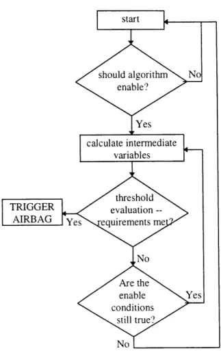
Figure 11: Flow Chart of the Algorithm

The algorithm first calculates and checks the enable signal. This is an indication of whether the a collision is occurring. If the enable signal is not asserted, the algorithm repeats the process by capturing and evaluating the next point. Once the collision has been detected, the algorithm is enabled and the main loop of evaluations starts.

Next, the intermediate values are calculated. These values include velocity, displacement, slope, energy, and more. There are other additional criteria including the rough road measures, the collision progression marker, and any other criteria which are used to assess the severity of the collision. Furthermore, these criteria are calculated in all three directions, unless there are cases in which these

(32)

criteria are unnecessary. For criteria such as the combined rectified energy, it becomes necessary to first calculate variables in each direction and combined using a fixed ratio.

Once all the intermediate values are calculated, they are compared against a set of calibrated thresholds. These thresholds are specially calibrated based on the platform of the vehicle. Since there may be 10-20 different criteria used, there are a few ways to derive the deployment decision based on these multiple criteria. First of all, the deployment decision can be based on crossing all of the thresholds

simultaneously. This is a very stringent condition which is aimed at eliminating unnecessary deployment of the airbag. However, there is always the possibility that not all of the criteria are met, even in a severe collision. Furthermore, in order to ensure all the criteria are met in a deploy event, the thresholds of the criteria have to be set at low levels. The thresholds must be kept low or else there is a risk that one of the thresholds is not crossed. Therefore, another approach is to allow the deployment decision to be based on only a fixed number of criteria which must cross the respective thresholds simultaneously. For example, instead of requiring all n thresholds are exceeded simultaneously, the deployment is valid if only (n-l) separate thresholds are crossed. This allows more leeway in calibrating the thresholds. However, as fewer thresholds are required to deploy the airbag, the repeatability and the validity of the algorithm begins to suffer. Another variation of this approach is to arbitrarily weigh the criteria used in the decision process. In other words, each criteria is assigned a number reflecting it's importance. At the end of the evaluation, the importance values of all the criteria which crossed the thresholds are added. The deployment decision will be based on the value of this final "score". This new extension serves one very

important purpose. It introduces intelligence by allowing the algorithm to pick and choose which criteria are needed for the deployment decision. However, there are also drawbacks. Certain criteria may be

essential for the deployment decision, and therefore these criteria must be given very high weight such

that the deployment is not possible unless these criteria are met.

Once the evaluation process is complete, the algorithm either asserts a deploy signal or it returns the control to the top of the algorithm and evaluates the next point. However, before the algorithm evaluates the next point, it first must check to see if the collision is still in progress. The collision progression measure is used to determine if the collision is still in progress. If the measure indicates that

(33)

the collision is still in progress, the algorithm fetches the next point and recalculate the intermediate variables. If the collision progression measure falls below the threshold, the control is returned to the top of the algorithm where it begins to look for the algorithm enable condition.

5.3. Performance Evaluation

5.3.1. Crash data

The crash data used for the evaluation is acceleration data from the actual vehicle crashes done at the vehicle test facility. In these controlled crashes, accelerometers are mounted on various locations of the vehicle to record the acceleration signals. For simplicity, the evaluation will be based on the acceleration signal collected from the accelerometers mounted near where the crash sensing module is placed. Furthermore, the crash data is obtained from a single platform of vehicle for reasons of consistency.

The categories of the crashes used for this evaluation are the following:

Full-frontal collisions:

* the vehicle is crashed into a non-deformable flat barrier at zero-offset and zero angle * various speed: 9mph, 12mph, 15mph, 30 mph, and 35 mph.

Angle collision:

* the vehicle is crashed into a non-deformable flat barrier which is placed such that the angle formed between the flat surface of the barrier and the bumper of the vehicle is at ±300.

* various speed: 12 mph, 15 mph, 30 mph. Pole collisions:

* the vehicle is crashed into non-deformable, cylindrical, high (telephone pole) and low (fire hydrant) pole at zero or percentage offset.

* various speed: 9 mph, 15 mph, 18 mph, 21 mph, 25 mph, 30 mph. Rough road events:

* uneven terrain: chatterbumps, potholes, bumps, * exterior events: hammer blow, door slam

(34)

The crash data is the raw acceleration read by the accelerometer. For each crash, the acceleration of the vehicle is recorded starting from the bumper contact (in some cases, however, the data is collected prior to the bumper contact) and continues to record for approximately 200-250 millisecond.

5.3.2. Procedure

The evaluation is done using a simulation tool. The tool simulates how the crash sensing module behaves when given the crash data collected from actual vehicle crashes done at the vehicle test facility.

Specifically, the tool is designed with a blackbox approach such that the end-user only needs to specify the input crash file. The results of the simulation are series of table and graphs. These tables and graphs show the activities of the algorithm by recording the time of all the events. The events include the enabling of the algorithm, the crossing of thresholds (both exceeding and falling below), and the time and the condition of trigger, if the deployment decision has been reached. In addition, the values of the intermediate variable (velocity, displacement, slope, etc.) throughout the entire evaluation interval are recorded. This information is helpful for optimizing the algorithm.

The original simulation tool was modified in order to accommodate the analysis of this project. The major change was in the input phase. Instead of using only the longitudinal acceleration signal, the input mechanism of the simulation tool had to be expanded to accept the lateral and the vertical

acceleration signals. Furthermore. the structure of the evaluation stage was expanded because new criteria had been added. Lastly, there were peripheral functions such as data collection and representation which must be modified for compatibility.

The results of the simulation details the performance of the algorithm. By examining the conditions and the timeliness of the deployment, the overall effectiveness and efficiency of the algorithm can be estimated.

(35)

5.3.3. Performance Requirements

5.3.3.1. Customer Requirements

The first step of the performance evaluation is to examine if all the customer requirements are met. These requirements are further broken down into two parts: the accuracy of the deployment decision,

and in the case of a deploy events, the timeliness of the deployment. The requirements are derived from the injury criteria established by the National Highway and Transportation Safety Authority1 6. In other words, the automotive manufacturers establish and adjust the requirements of each individual vehicle platform specifically to satisfy these injury requirements. The requirements for the vehicle platform under analysis, which are discussed in the next section, are used as the benchmarks for the evaluation.

There are several generalizations about the severity and the timing thresholds for the deployment of the airbag. First of all, the severity thresholds (the velocity which the airbag should be deployed) varies depending on the type of the collision. In the case of the full-frontal collisions of the vehicle under study, the velocity threshold for deployment is between 12 to 15 mph. The angle collision has a higher

deployment threshold at 20 mph. The pole collisions, which are difficult to detect, has a severity deployment threshold at 18 to 21 mph.

(36)

Crash type & velocity Frontal -9 mph 15 mph 30 mph 35 mph Angle -15 mph 20 mph 30 mph Pole - 14 mph 18 mph 21 mph 25 mph 30 mph deploy requirements no deploy deploy deploy deploy no deploy deploy deploy no deploy deploy deploy deploy deploy

goal time requirements N/A 50 ms 24 ms 18 ms N/A 44 ms 36 ms N/A 75 ms 75 ms 56 ms 43 ms

5.3.3.2. Comparison to the Single-Axis Algorithm

In addition to satisfying the customer requirements, the benefits of the new multi-axes algorithm cannot be shown unless the performance is compared against that of the single-axis algorithm. The criteria for comparison are discussed in the next section.

5.3.4. Criteria for Performance Evaluation

The following are the criteria used to evaluate the performance of the three-directional algorithm with respect to the single-directional algorithm. In general, these criteria are used to evaluate the

(37)

5.3.4.1. Accuracy

Accuracy refers to whether the algorithm has accurately distinguished the deploy events from the non-deploy events. This is the first pass of the evaluation process aimed at knowing if the algorithm has successfully identified the crashes which are near deployment thresholds. Once the accuracy of the algorithm is established, the performance of the deploy events are examined more carefully.

5.3.4.2. Timeliness

Timeliness refers to the time required for the algorithm to arrive at the deployment decision. Timeliness is not necessarily judged by how fast the deployment decision is made. The reason for that is

because the airbag should not be deployed much earlier than needed. First of all, the airbag is designed to inflate and deflate very quickly. After the airbag has fully inflated, the force of the body impacting the airbag should allow it to deflate quickly in order for the airbag to absorb the momentum of the moving body. If the airbag is inflated prematurely, it could have started to deflate by the time of the body contact. Therefore, while it is necessary to deploy the airbag within the time threshold, it is not necessary to make the decision as soon as possiblel7

The timeliness is judged by whether the deployment decision is made within the required time. However, to reach the deployment decision quickly is not necessarily useless. First of all, it increases the margin for errors. For example, if the deployment decision can be made very quickly, it is more likely

that the similar collisions are also detected on time. Second, if the decision has been arrived too quickly, an arbitrary delay can be imposed on the deployment signal. During the delay, the algorithm can

reconfirm the decision by continuing to evaluate the data until the end of the delay when the deployment

signal is asserted. If the evaluation of the data during the delay strongly suggests a non-deploy event, the deployment can be suppressed.

(38)

5.3.4.3. Robustness

Robustness ties in both the accuracy and the timeliness of the algorithm. It measures the performance of the algorithm if the original crash signals are altered. The crash signals are altered by multiplying the acceleration by a scale factor between 0.1 and 1.5.

Although changing the crash signal by multiplying it by a scale factor does not guarantee that the accuracy of the crash signal is preserved, it does, however, offer a new set of crash signals which carries some validity. For example, the crash signal of a 30 mph collision is multiplied by factors 0.9 and 1.1. It is true that these may not be the signals observed if the vehicle was crashed into the barrier at 27 mph and 33 mph, respectively, but they serve as estimations. One must keep in mind that the validity of the altered signal diminishes as the scale factor deviates farther away from 1.

To test the performance, the original crash signals are multiplied by factors from 0.1 to 1.5 with increments of 0. 1. Using simulation, these scaled signals are evaluated by the algorithm, and the accuracy and timeliness results are recorded. The evaluation is performed on the three-directional algorithm as well as the single-directional, controlled algorithm. The results are then compared.

(39)

Chapter 6 6. ANALYSIS/DISCUSSION

6.1. Correlation Method

Undoubtedly, the correlation methods relies heavily on the relationship between the signals from the different directions. If there are clear and consistent relationships between the signals, the correlation method allows one to make predictions about the unknown signals based on the known signals. However, the validity of the predictions depends heavily on the consistency of the relationships.

In this section, the analysis is aimed at establishing the relationships between the longitudinal, lateral, and vertical signals. Specifically, the analysis is focused on three groups of collisions, the frontal,

(40)

the angle, and the pole collisions. The goal of the method is to use the lateral and the vertical signals (the secondary signals) to assist the decision making processing which is based on the longitudinal signal (the primary signal).

6.1.1. Longitudinal versus Lateral

The focus of this analysis is to establish a relationship between the longitudinal and the lateral signals. One area where this relationship may be the strongest is the angle collision. Intuitively, the angle collisions have a significant lateral acceleration.

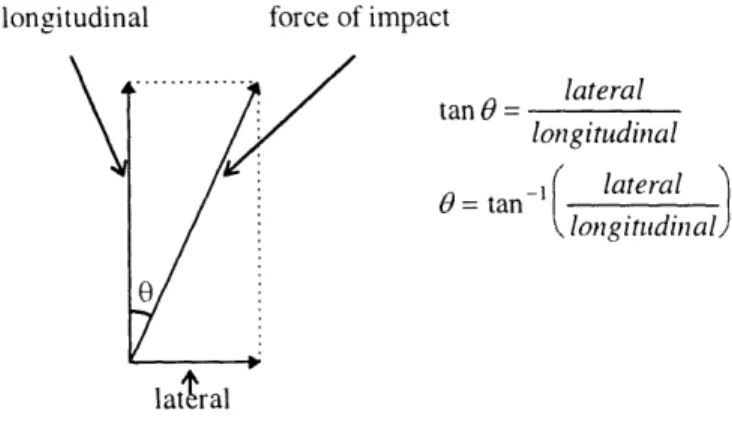
One method to establish the relationship is to analyze the angle of the collision. The algorithm can accurately determine the angle of the collision only if the relationship between the longitudinal and the lateral is valid (Figure 12). To test this hypothesis, the longitudinal and the lateral velocity signals of a 300 angle collision are used to derive the angle of the impact force.

longitudinal force of impact . tano= lateral longitudinal

O=tan -

lateral

Slongitudinal

lat'ral

Figure 12: Calculation of the angle of impact

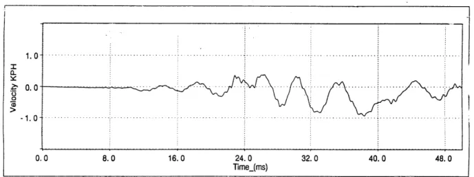
However, without the need to carry out any calculation, this method cannot accurately determine the angle of collision. The top graph is the lateral velocity of a frontal collision and the bottom graph is the lateral velocity of the 300 angle collision.

(41)

1.0-Lateral velocity of a 30 MPH frontal collision

Lateral velocity of a 30 MPH angle collision (barrier offset at 30 degrees)

Figure 18: Lateral Velocity -Frontal vs. Angle Collisions

The lateral velocity signal reveals a dip in the initial 15-20 milliseconds. Because of the change in the polarity of the velocity, the polarity of the angle of impact reverses. In addition, the calculated angle of impact is not accurate. At 15 millisecond into the collision, the longitudinal velocity is roughly 6 times larger than the lateral velocity, and the resolved angle is only approximately 14 degrees. The magnitude of the lateral velocity then begins to decrease which causes the angle to also decrease until the

h n.,,

(42)

sign of the angle is eventually reversed. At this time, the algorithm is required to reach the deployment decision. Because the calculated angle varies significantly up until the required time of deployment, the angle of the collision cannot be accurately determined by the required triggering time. Of the 10 high severity angle collisions analyzed, all shared the similar inconsistency.

Why did this method fail? Some speculations suggest that the energy transfer may not be consistent because of the structural components of the vehicle. By the time the impacting force has propagated through the vehicle to the accelerometer, the direction and the magnitude may have been dampened or altered. Another possible source causing the changes may be from the deformation. It is likely that the deformation of the main chassis also absorbs and alters the magnitude and the direction of the impacting force18

6.1.2. Longitudinal versus Vertical

Because the net displacement in the vertical direction is zero, it leads to the natural conclusion that the collision cannot have an impact vector which lies in the longitudinal-vertical plane. Therefore, instead of focusing on the direction of the impact, the analysis is based on the magnitude of the signals.

The plots of longitudinal and vertical velocity signals of frontal, angle, and pole collisions can be found in Appendix A. Plots 1. 4, and 7 are the longitudinal velocity signals of the frontal, angle, and pole collisions, respectively: plots 3, 6, and 9 are the vertical velocity signals of the frontal, angle, and pole

collisions, respectively. The velocity signals are chosen because of the intuition it provides and the ease to convert to either the acceleration or displacement signals.

The plots found in Appendix A consist of collisions of the same type at various speed. The focus of this analysis is only based on high speed collision, namely the 30-mph collisions. Consequently, the magnitude of the severity in all these collisions are the same. A quick look at the longitudinal velocities during the early part of the crashes when the discrimination against non-deploy events needs to be done reveals significant differences among the frontal, angle, and pole collisions. The longitudinal velocity of the frontal collision is clearly larger than those of the angle and the pole collisions in the first 20 to 50 milliseconds. The correlation method would suggest that the discrepancies may be compensated by the

(43)

vertical signals. However, a closer look at the vertical velocities of the respective collisions does not show that the differences in the longitudinal signals can be compensated. In the case of comparing the frontal to the angle collisions, the vertical velocity of the angle collision appears to be weaker than that of the frontal collision. Not only is the maximum velocity greater for the frontal collision, the area under the vertical velocity curve is also larger than that of the angle collision. Furthermore, the longitudinal

velocity of the pole collision is even weaker than that of the angle collision, and instead of compensating for this weakness, the vertical velocity is small compared to both the frontal and the angle collisions.

The conclusion of the simple analysis above reveals that for the collisions of the same degree of severity, the vertical signal does not compensate the differences in the longitudinal signals. Instead, the vertical signals are proportional to the magnitude of the longitudinal signals. Therefore, using the vertical

signals to compensate the longitudinal signals is not feasible.

6.1.3. Feasibility of the Algorithm

The analysis above shows very limited relationships between the longitudinal signals and both lateral and vertical signals. Although very specific correlation may exist between the variable, they are not global characterizations. For example, if a very specific, well-behaved relationship between the longitudinal and the lateral signals of the angle collision is discovered, the algorithm must first establish that the collision at hand is an angle collision before the correlation can be used. Consequently, the time required to establish the identity of the collision may be too long for the algorithm to be effective.

Without the predictable and reliable relationships between the variables, the correlation method is not feasible.

6.2. Rotated Axis Method

Rotated-axis method suggests that it may be possible to enhance the performance of the crash sensing algorithm if multiple accelerometers are placed at offset angles. If the method does suggest improvement in the performance, the question is what angle the accelerometers should be placed at.

(44)

6.2.1. Patents

There are several patents which describe crash detection methods using dual accelerometers placed at offset angle from the longitudinal axis or the direction of travel, one of which discusses how the crashes can be classified by using dual accelerometers placed at ±450 from the longitudinal axis'9. The

detection method relies on resolving the angle of the collision and deriving a threshold level based on the calculated angle of impact.

The analysis from the previous section concludes that the angle of collision cannot be accurately determined using longitudinal and lateral signals. Therefore, the question becomes: can the acceleration signals of the rotated-axis accelerometers provide a more accurate determination of the angle of impact? Following is the method used to determine the angle of impact described by the patent.

force of impact acceleration2 tan = aelera acceleraton 1 -= tn ' I rl 1 a = 450 -P acceleration 1 acceleration 2

Figure 14: Using Accelerometers placed at ±450 to Calculate the Angle of Collision

I acceeraton • '- " ",Lk a = 45°-fl "' I

~'l'll"

" ""'#l#; acceeraton

(45)

The algorithm calculates the angle of impact by finding the inverse tangent of the quotient between two raw acceleration signals. However, the validity of this approach is low because the raw acceleration signals are very noisy. When this approach was duplicated using the available raw crash data, the calculated angle varied inconsistently between 0 and 90 degrees.

6.2.2. Analysis

The results of the method described by the patent was not only difficult to duplicate, it did not contain additional information which was not available using longitudinal and lateral acceleration signals. The patented method relied on resolving the two acceleration signals to determine the angle and the magnitude of the impact force. Once the angle and the magnitude of the crash are known, the thresholds

for crash detection are adjusted accordingly. However, despite the fact that acceleration signals are noisy and the angle of impact cannot be accurately determined, there is no reason to believe that the results achieved by the offset accelerometers cannot be achieved by using the longitudinal-lateral pair of

accelerometers. Using the longitudinal-lateral pair of acceleration signals, the cosine law can also be used to determine the impact vector.

One benefit of the using a pair of accelerometers placed at ±0 degrees instead of the longitudinal-lateral pair is when the noise-to-signal ratio is large. To minimize the effects of this ratio, the magnitude of the original signal should be as large as possible. Therefore, placing the accelerometers in the direction of the impact may maximize the magnitude of the crash signal. However, the energy transfer must be consistent throughout the vehicle such that in an angle collision, the angle of impact can be recovered by resolving the signals of the accelerometers. In other words, it may be possible that due to the structural deformation or the inconsistent energy transfer that the angle seen by the accelerometers is not the same

angle as the angle of impact-o. In addition, to place the accelerometers at an offset angle to better detect the angle collisions inevitably sacrifices the effectiveness in detecting the full frontal collisions. If the accelerometers are placed at ±450 with respect to the longitudinal axis, a frontal collision would therefore be recognized only with approximately 70%c of the signal amplitude. Consequently, the threshold must

(46)

also be lowered by 70%. Assuming that the magnitude of the noise remains constant, the noise-to-threshold ratio becomes larger.

One can also argue that the rotated-axis method improves reliability of the algorithm"2. Because each of the two accelerometers placed at ±450 with respect to the longitudinal axis contains both

longitudinal and lateral information, the crash sensing unit can be functional even if only one accelerometer is present. However, the complexity increases if the crash sensing algorithm must be functional with both single and dual accelerometers. Furthermore, the robustness of the algorithm is seriously damaged if only one accelerometer remains, and inevitably, the crash sensing unit must be replaced immediately.

The rotated-axis method cannot better determine the angle of impact of a collision. However, it provides addition lateral information which is not available in the single-directional sensing strategy. One can further conclude that the while the rotated-axis method generates the lateral information which can be treated as an independent component and analyzed separately, the same information can be obtained using accelerometers placed along longitudinal and lateral axis of the vehicle. In conclusion, the rotates-axis method does not provide additional information which is not available using the independent threshold method with the longitudinal-lateral pair of accelerometers. The independent threshold method is discussed in the following section.

6.3. Independent Threshold Method

Because the above two methods are not feasible or practical, the focus of the thesis is on the independent threshold method discussed here. The results and the evaluation are based solely on this algorithmic approach.