Exploring the potential for energy conservation in French households through hybrid modelling

HAL Id: hal-00866425

https://hal.archives-ouvertes.fr/hal-00866425

HAL is a multi-disciplinary open access archive for the deposit and dissemination of sci-entific research documents, whether they are pub-lished or not. The documents may come from teaching and research institutions in France or abroad, or from public or private research centers.

L’archive ouverte pluridisciplinaire HAL, est destinée au dépôt et à la diffusion de documents scientifiques de niveau recherche, publiés ou non, émanant des établissements d’enseignement et de recherche français ou étrangers, des laboratoires publics ou privés.

Exploring the potential for energy conservation in

French households through hybrid modelling

Louis-Gaëtan Giraudet, Céline Guivarch, Philippe Quirion

To cite this version:

Louis-Gaëtan Giraudet, Céline Guivarch, Philippe Quirion. Exploring the potential for energy con-servation in French households through hybrid modelling. 2011. �hal-00866425�

C.I.R.E.D.

Centre International de Recherches sur l'Environnement et le Développement

UMR

8568

CNRS

/

EHESS

/

ENPC

/

ENGREF

/

CIRAD /

M

F

45 bis, avenue de la Belle Gabrielle

F-94736 Nogent sur Marne CEDEX

Tel : (33) 1 43 94 73 73 / Fax : (33) 1 43 94 73 70

www.centre-cired.fr

DOCUMENTS DE TRAVAIL / WORKING PAPERS

No 26-2011

Exploring the potential for energy conservation

in French households through hybrid modelling

Louis-Gaëtan Giraudet

Céline Guivarch

Philippe Quirion

Exploring the potential for energy conservation in French households through hybrid modelling

Abstract

Although the building sector is recognized as having major potential for energy conservation and carbon dioxide emissions mitigation, conventional bottom-up and top-down models are limited in their ability to capture the complex economic and technological dynamics of the sector. This paper

introduces a hybrid framework developed to assess future household energy demand in France. Res-IRF, a bottom-up module of energy consumption for space heating, has several distinctive features: (i) a clear separation between energy efficiency, i.e. investment in energy efficient technologies, and sufficiency, i.e. changes in the utilization of energy consuming durables which allows the rebound effect to be assessed; (ii) the inclusion of barriers to energy efficiency in the form of intangible costs, consumer heterogeneity parameters and the learning-by-doing process ; (iii) an endogenous

determination of retrofitting which represents trade-offs between retrofit quantity and quality. Subsequently, Res-IRF is linked to the IMACLIM-R computable general equilibrium model. This exercise shows that, compared to a 37% reduction in final energy demand achievable in business as

usual in existing dwellings, an additional reduction of 14% could be achieved if relevant barriers to

efficiency and sufficiency were overcome.

Keywords : Hybrid modeling, Residential heating, Barriers to energy efficiency, Rebound effect,

Endogenous retrofitting dynamics, Intangible costs.

Exploration du potentiel de maîtrise de l’énergie des ménages français par la modélisation hybride

Résumé

Le secteur du bâtiment est reconnu comme le principal gisement d’économies d’énergie et de réduction des émissions de dioxyde de carbone. Toutefois, les méthodes conventionnelles

d’évaluation bottom-up et top-down ne permettent pas de prendre en compte de façon satisfaisante les dynamiques économiques et technologiques complexes qui le caractérisent. Cet article présente un modèle hybride spécifiquement développé pour évaluer la demande d'énergie future des ménages français. Res-IRF, un module bottom-up de consommation de l'énergie pour le chauffage, est construit avec les caractéristiques suivantes : (i) une séparation nette entre les comportements d'efficacité énergétique, i.e. investissement dans les technologies efficaces, et de sobriété, i.e. variation de l’utilisation des équipements, qui permet d'évaluer l’effet rebond ; (ii) l'inclusion de barrières à l'efficacité énergétique sous la forme de coûts intangibles, de processus d'apprentissage et de paramètres d'hétérogénéité des ménages ; (iii) une détermination endogène du processus de rénovation, qui représente un arbitrage entre le nombre et la qualité des rénovations. Res-IRF est couplé au modèle d'équilibre général calculable IMACLIM-R, adapté à l’économie française. Les simulations prospectives montrent que, comparée à une réduction de 37 % de la demande d'énergie finale en business as usual, une réduction additionnelle de 14 % peut être atteinte si les barrières qui s’opposent à l'efficacité et la sobriété sont surmontées.

Mots-clés: modélisation hybride, chauffage résidentiel, barrières à l’efficacité énergétique, effet

1

Exploring the potential for energy

conservation in French households

through hybrid modelling

Louis-Gaëtan Giraudeta,b,*, Céline Guivarcha,b, Philippe Quirionc,b

Abstract

Although the building sector is recognized as having major potential for energy conservation and carbon dioxide emissions mitigation, conventional bottom-up and top-down models are limited in their ability to capture the complex economic and technological dynamics of the sector. This paper introduces a hybrid framework developed to assess future household energy demand in France. Res-IRF, a bottom-up module of energy consumption for space heating, has several distinctive features: (i) a clear separation between energy efficiency, i.e. investment in energy efficient technologies, and sufficiency, i.e. changes in the utilization of energy consuming durables which allows the rebound effect to be assessed; (ii) the inclusion of barriers to energy efficiency in the form of intangible costs, consumer heterogeneity parameters and the learning-by-doing process ; (iii) an endogenous determination of retrofitting which represents trade-offs between retrofit quantity and quality. Subsequently, Res-IRF is linked to the IMACLIM-R computable general equilibrium model. This exercise shows that, compared to a 37% reduction in final energy demand achievable in business as

usual in existing dwellings, an additional reduction of 14% could be achieved if relevant barriers to

efficiency and sufficiency were overcome.

Keywords

Hybrid modeling, Residential heating, Barriers to energy efficiency, Rebound effect, Endogenous retrofitting dynamics, Intangible costs

a

Université Paris-Est, Ecole des Ponts ParisTech. Marne-la-Vallée, France

b

Centre international de recherche sur l’environnement et le développement (CIRED). Nogent-sur-Marne, France

c

Centre national de la recherche scientifique (CNRS). Paris, France

* Corresponding author : CIRED, 45 bis avenue de la Belle Gabrielle, F-94736 Nogent sur Marne Cedex. Tel : +331.43.94.73.62. E-mail : giraudet@centre-cired.fr

2

1 Introduction

Until the last decade, the debate in energy-economy modelling was polarised between economists’ top-down and engineers’ bottom-up techniques. Since then, so-called “hybrid” models have been used, in some sectors, to combine the technological explicitness typically found in bottom-up models with the economic mechanisms typically found in top-down models (Hourcade et al., 2006). To date, hybrid models have focused on electricity generation and, to a lesser extent, on transportation, but rarely on the building sector1, in spite of its major potential for energy conservation and carbon dioxide emissions mitigation (Levine et al., 2007). Yet hybrid modelling represents a promising tool for addressing the complex economic and technological dynamics in this sector, which conventional bottom-up or top-down models fail to capture.

The first weakness, frequently pointed out in conventional modelling, is the emphasis placed on technology adoption rather than technology utilization (Ürge-Vorsatz et al., 2009; Moezzi et al., 2009; Kavgic et al., 2010). Energy conservation can be seen as the interplay between efficiency, i.e. investment in energy efficient technologies, and sufficiency, i.e. a decrease in the utilization of energy consuming durables (Herring, 2009; Alcott, 2008). The former has received more attention from forward-looking studies, but the latter must also be included to fully assess the potential for energy conservation. Furthermore, considering together efficiency and sufficiency allows the rebound effect to be addressed (Sorrell and Dimitropoulos, 2008; Sorrell et al., 2009), i.e. when energy efficiency improvements are followed by a less-than-proportional decrease (or even increase) in absolute energy consumption due to increased load or frequency of use of the equipment.

Although efficiency has been prioritized, conventional models have failed to satisfactorily address the “energy efficiency gap” (Jaffe and Stavins, 1994b; Sanstad and Howarth, 1994), i.e. the under-provision in energy efficient durables despite the social profitability of such investments. Purchase decisions are subject to a set of “barriers”, categorized either as market failures that blur cost-minimizing investment decisions, e.g. imperfect information, split incentives or liquidity constraints, or behavioural failures, such as bounded rationality and heuristic decision-making, that move investment decisions away from cost-minimization (Gillingham et al., 2009; Sorrell, 2004). Pure top-down models tend to ignore the gap, whereas pure engineering bottom-up models tend to overestimate it (Hourcade et al., 2006). Between the two, the problem is generally restated, rather than directly addressed, by using particularly high discount rates to represent the whole set of barriers (Jaffe and Stavins, 1994a,b; Mundaca, 2008).

The aim of this paper is to introduce a hybrid framework specifically developed to overcome these problems. It builds on the connection of Res-IRF, a bottom-up module of the French building stock, to the general equilibrium model IMACLIM-R (Crassous et al., 2006; Sassi et al., 2010) adapted to France. Res-IRF focuses on the consumption of electricity, natural gas and fuel oil for space heating2 which accounts for 20% of total French energy consumption (ADEME, 2008). It is designed with a

1 _{Hybrid models addressing residential buildings include CIMS in Canada (Jaccard and Dennis, 2006), Hybris in} Denmark (Jacobsen, 1998) and NEMO-ICARUS in the Netherlands (Koopmans and te Velde, 2001).

3

flexible simulation architecture which allows the incorporation of insights from both engineering and various economic fields. The overall modeling framework can be regarded as hybrid3 in two ways: (i) Res-IRF is a bottom-up model enriched with microeconomic mechanisms; (ii) its linkage to IMACLIM-R France ensures macroeconomic consistency.

This paper considers the questions: How can the major barriers to energy conservation be

represented in a hybrid model? What potential for energy conservation is hindered by such barriers?

Section 2 describes the simulation module and the grounds for modelling choices. Section 3 analyses a reference scenario to illustrate the basic phenomena addressed by Ref-IRF. Section 4 provides a sensitivity analysis that allows quantifying the potential for energy conservation in existing dwellings. Section 5 concludes.

2 The Residential module of IMACLIM-R France (Res-IRF)

Res-IRF models the evolution of building stock energy performance through new constructions, energy retrofits and fuel switches4. This section comments on the main equations of the model; the parameter settings are outlined in annex 1.

2.1 Determinants of the demand for space heating

At the most aggregate level, the final energy demand for space heating (Efin, in kWh/year) can be

decomposed as a product of total building stock (S, in m²), an “efficiency” term (Econv/S) in

kWh/m²/year) standing for specific energy consumption under conventional utilization, and a “sufficiency” term, or dimensionless service factor (Efin/Econv) representing the continuous short-term

adjustment of heating infrastructure utilization. This is summarized by the following identity:

fin conv fin conv

E

E

E

S

S

E



(S) is made up of “existing” buildings, i.e. those standing prior to the calibration year 2007, and “new” buildings, constructed from 2008 onwards. Both stocks are disaggregated into detached houses and collective dwellings, by energy carrier (electricity, natural gas, fuel oil) and by energy performance class. The heating infrastructure is not described explicitly, but implicit packages of measures on the building envelope (insulation, glazing) and the heating system are assumed to reach discrete levels of energy efficiency. The performance of the existing building stock ranges from class G, the least efficient (over 450 kWh/m²/year of primary energy for heating, cooling and hot water) to class A, the most efficient (below 50 kWh/m²/year of primary energy), as labelled by the French

3 _{Hourcade et al. (2006) define hybrid models as “those bottom-up or top-down energy-environment models} that have made at least one modification that shifts them substantially away from their conventional placement [along the three dimensions of technological explicitness, microeconomic realism and macroeconomic completeness+”.

4 _{Hence, it features a “putty-semi-putty” capital specification, stating that capital malleability is higher ex ante} than ex post (Koopmans and te Velde, 2001).

4

energy performance certificate (Marchal, 2008; MEEDDAT, 2008). The new building stock is split into three performance categories: the ‘BC05’ or building code 2005 level (from 250 to 120 kWh/m²/year of primary energy, depending on the local climate, for heating, cooling, hot water and ventilation), ‘LE’ or Low-Energy buildings (50 kWh/m²/year) and ‘ZE’ or Zero-Energy buildings for which primary energy consumption is lower than the renewable energy they can produce (MEEDDM, 2010). After denoting I={G,...,A} the set of efficiency classes in existing dwellings, J={BC05, LE, ZE} the set of construction categories, ρk a parameter representing the inverse efficiency of class k and Fk a variable

representing the service factor of class k, identity (1) can be restated as:

fin k k k k I J

E

S



F

 





This equation is very similar to those used for energy demand relations in conventional models (Jacobsen, 1998; Swan and Ugursal, 2009). The association of the last two terms follows a classical discrete-continuous approach (Hausman, 1979 ; Dubin and McFadden, 1984 ; Nesbakken, 2001). Section 2.2 concentrates on the retrofitting process that determines

 

 

determined in a very classical manner by population and income growth, is described in annex 3.

2.2 Retrofitting dynamics

Retrofits are modelled as transitions from an initial efficiency class i (iI) to any higher final class f ( f I f, i). Overall, energy efficiency improvements in existing dwellings come from variations in the quantity and/or the quality (i.e. the ambition) of retrofits; both derive from changes in the relative profitability of retrofitting options. Such variations are induced by energy prices and sustained by retrofitting cost decreases. The latter is consecutive to the self-reinforcing processes of information acceleration on the demand side and learning-by-doing on the supply side. Finally, this evolution is countervailed by the natural exhaustion of the potential for profitable retrofitting actions. The general dynamics is mediated by parameters reflecting consumer heterogeneity and some barriers to energy efficiency.

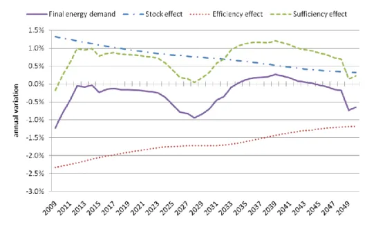
The equation system determining the retrofitting dynamics is mapped in figure 1 and developed hereafter. Note that without explicit temporal subscript, variables hold at the year considered.

5

Figure 1: The retrofitting dynamic system

The dashed box delineates stock Si(t+1). Above are classes f>i and below are classes k<i. Dotted

arrows indicate how input variables enter the system. Thin arrows refer to other deterministic relations. Thick arrows indicate physical flows of dwellings that quit or enter stock Si(t+1). Capital

letters refer to variables and small ones to main parameters.

2.2.1 Capital turn-over

Each year, the building stock Si is eroded by demolition of a fraction γi of class i dwellings. Following

Sartori et al. (2009), this process is assumed to affect the worst energy classes first. In addition, stock

Sigains some dwellings that are retrofitted from any lower class k (kI k, i) to class i, and loses

some dwellings retrofitted to any higher energy class f ( f I f, i):

, ,

(

1)

(1

) ( )

(

1)

(

1)

S t



S t

TRANS

t

TRANS

t

  





 





being chosen in proportion PRi,f :

,

(

1)

(1

) ( )

(

1)

(

1)

i f i i i i f

TRANS

t

  



S t X t



PR

t



(4)

2.2.2 Choice of a retrofitting option

The proportion PRi,fof class i dwellings that are retrofitted to higher classes f is inferred from the life

cycle cost of the transition compared to the life cycle costs of all other possible transitions to higher classes h (hI h, i): , , , i f i f i h h i

LCC

PR

LCC





6

Life cycle costs are the sum of transition costs CINVif, lifetime energy operating expenditures

CENERfborne in final class f and intangible costs ICif :

, , ,

i f i f f i f

LCC



CINV



CENER



IC

(6)

Equation 5 is inspired by the CIMS model (Rivers and Jaccard, 2005; Jaccard and Dennis, 2006). It incorporates a positive parameter ν, implying that the lower the life cycle cost of one transition compared to all others, the higher its proportion. Moreover, ν allows allocating a non-null market share to each option, hence overcoming the simplistic representation of a “mean householder” choosing exclusively the least life cycle cost option. In other words, ν reflects the heterogeneity of markets and preferences, provided that people might be randomly interested in some attributes of the technology other than energy efficiency. In Res-IRF, ν is set exogenously to 8 which allocates a 44% proportion to the least-cost transition departing from class G.

2.2.3 Transition costs and learning-by-doing

Numerous possible combinations of measures on the envelope and the heating system are abstracted into a limited number of average transition packages. However, information about implicit transition costs is less readily available than information about underpinning technology costs. To cope with lacking data, the matrix of initial transition costs CINVif(0), i.e. the sum of

equipment purchase and installation cost, is constructed with respect to the following principles: (i) retrofitting has marginally decreasing returns (BRE, 2005), i.e. the marginal cost of reaching the next more efficient class is increasing; (ii) some technical synergies make it more profitable to co-ordinate measures rather than to undertake them successively (Gustafsson, 2000), i.e. the cost for one direct transition (e.g. from i to f) is lower than for any combination of smaller successive transitions leading to an equivalent upgrade (e.g. from i to an intermediate class k to f); (iii) retrofitting a very inefficient dwelling is roughly as costly as destructing and reconstructing it, i.e. the cost of transition G to A is slightly below the cost of a new construction, which is around €1,200/m² (MEEDDM, 2010).

Final energy class (f)

F E D C B A Initial energy class (i) G 50 150 300 500 750 1,050 F 110 260 460 710 1,010 E 170 370 620 920 D 230 480 780 C 290 590 B 350

7

A variable share α of transition costs is subject to learning-by-doing, i.e. cost decrease with experience accumulated over time. This process is implemented as a classical power function (Wing, 2006; Gillingham et al., 2008), parameterized by a learning rate l, which controls for the cost decrease induced by a doubling of cumulative experience Kf :

log( ( ) (0)) log 2 ,

( )

(0)

(1

)(1

)

CINV

t

CINV





l











 











The same variable Kf applies to all transitions to final class f, whatever the initial class i, hence

assuming implicit spillovers among transitions leading to the same final class. Cumulative experience

Kf is approximated as the sum of past transitions to final class f :

,

(

1)

( )

(

1)

K t

K t

TRANS

t

 







Learning-by-doing is well established for energy supply technologies, but less for the more diverse end-use technologies (Laitner and Sanstad, 2004; Jakob and Madlener, 2004). Yet a recent review of empirical works tends to show that learning rates for end-use technologies are around 18+/-9%, which is close to those historically estimated for supply technologies (Weiss et al., 2010). Setting learning rate values in Res-IRF from these empirical estimates is challenging in two ways. First, the technological abstraction of energy class transitions raises the tricky issue of how to aggregate the learning rates of underpinning technologies (Ferioli et al., 2009). Second, empirical estimates are derived from technology purchase prices, hence abstracting from installation costs that might be high and less likely to decrease. Accordingly, Res-IRF assumes modest learning rates, as is further developed in annex 1.

2.2.4 Myopic expectation and heterogeneous discounting

Res-IRF incorporates “myopic expectation”, i.e. annual streams of energy operating expenditures borne in class f of inverse efficiency ρf are valuated at current energy prices P (assuming unchanged

energy carrier), projected over the lifetime n of the investment and discounted at rate r :

1 (1

)

( )

r

CENER P

P

r





 



 







This assumption, shared by most models of household energy demand5, is primarily driven by technical constraints. According to Jaffe and Stavins (1994a), myopic expectation has been used routinely for estimating discount rates in a context of under-determined observations6. Furthermore,

5 _{Note that the inverse calculation, i.e. weighting annual energy costs against the investment annuity, is} generally used. See for instance Dubin and McFadden (1984, p.350-1).

6 _{“The effects of [the energy price] and [the discount rate] are indistinguishable from each other. [...]. In} practice, we cannot measure either of these. So instead, what is typically done is to [...] assume that [the

8

the alternative assumption of perfect foresight is difficult to implement in recursive simulation models such as Res-IRF. It is a fortiori not realistic and theoretical grounds for using myopic expectations can be invoked, compatible with various market barriers or behavioural failures. Some authors see it as a reaction to uncertainty about the future energy prices (Hassett and Metcalf, 1993). Others refer to “folk quantification of energy” as Kempton and Montgomery (1982), who bring that feature under the heading of bounded rationality.

Private discount rate estimates for insulation and space heating investments typically reach 20-25% (Hausman, 1979; Dubin and McFadden, 1984; Train, 1985; Metcalf and Hassett, 1999; see Mundaca, 2008, Annex A.2, for the most up-to-date review). Such high values compared to conventional household investments have been interpreted as a manifestation of the energy efficiency gap (Sanstad and Howarth, 1994). As such, they are just “a restatement of the phenomena to be explained”, namely the multiple barriers to energy efficiency investments (Jaffe and Stavins, 1994b, p.807; Sorrell, 2004, p.31). Res-IRF leans on the discount rate to illustrate some of the barriers, but not all. Indeed, heterogeneous discount rates are used to account for the ‘landlord-tenant dilemma’. This refers to the split-incentives faced by the owner and the renter of a dwelling: the former is unable to recover energy efficiency investments whose benefits will accrue to the latter; the renter is neither able to recover investments whose paybacks are longer than his typical occupancy period. This phenomenon is confirmed by the observation that rented dwellings consume more energy than owner-occupied ones (Scott , 1997, for Ireland; Leth-Petersen and Togeby, 2001, for Denmark; Levinson and Niemann, 2004, in the U.S.; Rehdanz, 2007, for Germany).

Against this background, Res-IRF assumes that homeowners who face the dilemma (i.e. non-occupying ones) have higher profitability requirements for energy efficiency investments (i.e. higher discount rates) than those who do not (i.e. occupying homeowners)7. This discrepancy is further split with respect to the type of dwelling. Owners of detached houses are assumed to be more willing to undergo energy efficiency investments (i.e. have lower discount rates) than owners of collective dwellings, who may be discouraged by condominium rules or the imperfect appropriation of energy savings due to heat transfers with adjacent dwellings. Following these principles, numerical values shown in table 2 are set in Res-IRF so as to (i) assign a conventional private discount rate of 7% to agents that are the most likely to invest, i.e. occupying homeowners, and (ii) allow the average discount rate weighted by the share of each type of investor to match the ‘credit card’ value of 21% commonly estimated for energy efficiency investments. Such a method implies that only a fraction of the population might be responsive to policies (IEA, 2007).

energy price] is equal to the current price, and then estimate the discount rate *...+.” (Jaffe and Stavins, 1994a, p.50)

7 _{This tentative way of addressing the ‘landlord-tenant dilemma’ leaves aside some important issues. It} abstracts from the reimbursement of the investment via possible gains on the real estate value of the dwelling (Jaffe and Stavins, 1994a; Scott, 1997). Moreover, it does not take into account the “sufficiency” side of the dilemma, which arises in cases where energy bills are included in the rent, hence reducing the renters’ incentives to lower utilization (Levinson and Niemann, 2004). Those issues are a fruitful area for further research and modelling.

9

Detached house Collective dwelling

Owner-occupied 45% ; r = 7% 12% ; r = 10%

Rented 11% ; r = 35% 32% ; r = 40%

Table 2: Numbers (as % of the total stock) and discount rates (in %/year) in each type of dwelling

2.2.5 Intangible costs and information acceleration

Leaning solely on financial costs CINVi,f and CENERf to determine the proportion of transition PRi,f

(equations 5 and 6) would not necessarily allow reproducing the transitions observed in reality. Indeed, there is empirical evidence in France for a straight mismatch between the rankings of energy efficiency options according to their pure financial cost and their relative realisation (Laurent et al., 2009). Likewise, a French household survey showed that when people were asked about the main reason for which they had undergone energy efficiency actions, ‘alleviating fuel bill’ covers only 27% of the answers (TNS Sofres, 2006, p.33). Res-IRF copes with this difficulty by adding to financial costs some “intangibles costs”, as extensively used in the CIMS model (Rivers and Jaccard, 2005; Jaccard and Dennis, 2006), in order to reproduce the energy class transitions observed in 2008. The calibration of initial intangible costs is detailed in annex 4. Intangible costs appear as a convenient abstraction for the monetization of all the determinants of energy investment decisions that remain unexplained by direct financial costs. Interpreting them in the light of economic theory is more challenging, but they can be seen as partially expressing imperfect information, recognized as the major market failure that prevents energy efficiency investments (Ürge-Vorsatz et al., 2009).

In a dynamic perspective, there is compelling evidence from various fields of social science, such as behavioural economics, public policy evaluation or marketing (see Wilson and Dowlatabadi, 2007) that information about technology adoption spills over with cumulative experience8, thus inducing positive externalities that might justify public intervention (Jaffe and Stavins, 1994a, Jaffe et al., 2004). Following CIMS model (Mau et al., 2008; Axsen et al., 2009), this process is represented in Res-IRF as decreasing intangible costs ICi,f with cumulative capital stock Kf of final class f (as

introduced in equation 8). Hence, as intangible costs decrease, the proportion of energy class transitions become increasingly determined by sole financial costs (thus ameliorating the quality of retrofits). This process is bounded by a share β of fixed intangible costs, representing, for instance, the inconvenience due to indoor insulation works (Scott, 1997). The remaining share of variable intangible costs follows a logistic fit parameterized by c>0 and d>0, both expressed as a combination of β and the “information rate” u. Like the learning rate in the learning-by-doing process, parameter

u controls for the magnitude of intangible cost decrease induced by a doubling of the capital stock:

8 _{This process is labelled in many different ways, such as “learning-by-using” (Jaffe et al., 2004; Gillingham et}

al., 2009), “social contagion” (Mahapatra and Gustavsson, 2008), “social learning” (Darby, 2006a) or “the

neighbour effect” (Mau et al., 2008; Axsen et al., 2009). Among other factors, it builds on the fact that investments in energy efficiency have a socially distinctive, cumulative function (Maresca et al., 2009). Empirical quantification of the phenomenon is scarce, but tends to handle it as a logistic process (e.g. Darby, Axsen et al., Mau et al.).

10 , ,

1

( )

(0)

( )

1

exp

(0)

1

with

(1

)(1

) exp(1) and

1

IC

t

IC

K t

c

d

K

c

u

d

c



























_



_







_

_

_









_

_







 







2.2.6 Endogenous retrofitting rate

Upgrading the energy performance of an existing dwelling implies a binary decision about whether or

not to retrofit, inextricably linked to the discrete choice of an energy efficiency option (Cameron,

1985; Mahapatra and Gustavsson, 2008; Banfi et al., 2008). Modelling efforts tend to focus on the latter decision, holding the former exogenous (e.g. Siller et al., 2007). Res-IRF deals with this issue by computing endogenously the fraction Xi of the remaining stock (1-γi)Si that is upgraded annually (see

equation 3). For each initial energy class i, Xiis deduced from the “net present value of retrofitting”

NPVi (in euro per dwelling) by a sigmoid curve parameterized by a>0 and b >0:

,

1

(

)

1

exp(

)

X

f

NPV

a

bNPV









The net present value of retrofitting is the difference between energy operating expenditures borne in the current energy class CENERiand the life cycle cost of an average retrofitting project, i.e. the

sum of the life cycle costs LCCi,f of all possible transitions, weighted by their respective proportion

PRi,f : , , i i i f i f f i

NPV

CENER

PR LCC







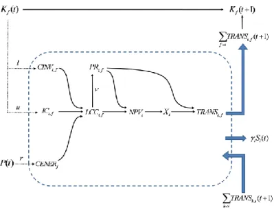
This specification makes the net present value, and thus the retrofitting rate, responsive to economic factors such as energy prices. The sigmoid curve implies that the more profitable the retrofitting (i.e. the higher the net present value), the larger the fraction of retrofitted dwellings. The curve used in figure 2 is calibrated by selecting the positive values of a and b that minimize the realisation of retrofitting projects with null net present value9, subject to the reproduction of total retrofits10

TRANS0 observed for year 0 (2007):

9 _{Since the sigmoid is monotonically increasing, this is a sufficient condition for minimizing the realisation of all} retrofitting projects with a negative net present value. Some unprofitable projects are undergone – in tiny numbers though –, which prevents discontinuities in the retrofitting process.

10 _{This refers exclusively to the significant retrofits that induce transitions by at least one energy class. The total} retrofitting activity is quite stable at 11% of the building stock per year in France, but dominated by basic

11 , , 0 0 0 ,

(0)

. .

(

)

. .

0,

0

Min f

s t

S f

NPV

TRANS

s t a

b





_







_

_





Figure 2: Share of retrofitted dwellings with respect to the net present value of retrofitting

2.3 Sufficiency and the rebound effect

Once new energy-consuming capital is embodied in new and existing buildings, one can observe systematic deviations between effective energy consumption Efinand the energy Econv that should be

consumed under the conventional assumptions set by performance labels (efficiency classes I and construction categories J), e.g. setting thermostat to 19°C. This gap stems from technical defects (Sanders and Phillipson, 2006) and more importantly from individual variations in the utilization of the heating infrastructure (Cayla et al., 2010). Such behavioural change is underpinned by economic and non-economic determinants (Ürge-Vorsatz et al., 2009). The former refers to rational responses to economic signals such as the price of the energy service (derived from the price of equipments and energy inputs), which gives rise to the direct rebound effect11 (Sorrell and Dimitropoulos, 1998). The latter refers to psychological, cultural or lifestyle determinants that are still poorly known but increasingly analysed (Maresca et al., 2009; Subrémon, 2010).

measures that do not yield energy efficiency gains, like wall painting. Overall, it is estimated that only 1% of the building stock has received measures leading to effective and significant energy savings in 2007 (OPEN, 2008).

11

At the microeconomic level, the direct rebound effect operates as follows: “Improved energy efficiency for a particular energy service will decrease the effective price of that service and should therefore lead to an increase in consumption of that service. This will tend to offset the reduction in energy consumption provided by the efficiency improvement” (Sorrell and Dimitropoulos, 2008, p.637). Note that this mechanism abstracts from income effects.

12

Ref-IRF focuses on the economic determinants of capital utilization or “sufficiency”. These are, at best, considered in bottom-up models through a price elasticity of the demand for energy service12. Shortcomings stem from holding elasticity constant, whereas such a relation is unlikely to be isoelastic (Haas and Schipper, 1998). In contrast, Res-IRF builds on a logistic relation that links the “service factor” or utilization variable F (which reflects the gap between effective and conventional energy consumption Efin/Econv) to the annual heating expenditure, as a proxy for the price of the

heating service. For any dwelling of class k (k I J ), the annual heating expenditure being the product of inverse efficiency parameter ρk and energy price input P, variable Fkis defined as follows:

0.7

( )

1.16 0.35

11

1 4 exp

2

F P

P



























_









_

_







This relation is empirically established for space heating in France by Allibe (2009), following an original specification of Haas et al. (1998). It states that the higher the efficiency of the dwelling (i.e. the lower ρk), the higher the service factor, thus inducing sufficiency relaxation. Conversely, the

higher the energy price, the lower the service factor, thus inducing sufficiency strengthening. Both efficiency and energy price effects are illustrated in figure 3 for the main efficiency classes and fuel types13. Along one single curve, investments that move a dwelling from a domain of low efficiency to a domain of a higher one (e.g. from class F to class C) increase the service factor, i.e. induce a rebound effect. Similarly, switching from a certain energy carrier to one fuelled by a cheaper energy (e.g. from oil to gas) within the same efficiency domain implies a vertical shift from a sharp curve to a gentler one, determining a higher service factor. More generally, any decrease in energy price stretches the curve (i.e. lowers the steepness at one point), thus raising the service factor, even though the fuel and efficiency of the energy carrier remain unchanged. The opposite occurs if energy price increases.

12 _{In top-down models, behavioural changes are generally merged together with efficiency improvements into} price and income elasticities of the demand for energy.

13 _{For the purpose of illustration, figure 3 expresses the service factor as a function of efficiency, which takes} continuous values on the x-axis, parameterized by the 2008 prices of the three main fuels. In Res-IRF, however, the efficiency parameter takes discrete values, as specified in equation 14, and the service factor fits a step curve.

13

Figure 3: Sufficiency curve (adapted from Allibe, 2009)

2.4 IMACLIM-R macroeconomic feedback

Overall, the household energy demand system encapsulated in Res-IRF is determined by three input variables: the energy price P, which determines efficiency and sufficiency behaviours (see equations 9 and 14), population L and disposable income Y, which both determine the growth of the total building stock (see annex 3). In a broader perspective, Res-IRF is recursively connected to the computable general equilibrium model IMACLIM-R (Crassous et al., 2006; Sassi et al., 2010), adapted to France as a small open economy. Within this hybrid framework, energy prices and disposable income are endogenous variables: according to figure 4, disposable income and energy prices are solved at year (t) in the static equilibrium module of IMACLIM-R, then sent as inputs to Res-IRF, which in turn generates new demands for investment and energy that are ultimately used to compute income and energy prices in the static equilibrium at year (t+1).

Therefore, the retroaction of Res-IRF over the general equilibrium affects only energy markets and household consumption. Note that disposable income increases the total building stock, but it has no direct effect on efficiency and sufficiency behaviours in Res-IRF. Population growth is an exogenous variable for both IMACLIM-R France and Res-IRF.

14

Figure 4: Recursive connection of Res-IRF to IMACLIM-R France

3 Business as usual scenario

Res-IRF is run to provide a reference or business as usual scenario, assuming constant climate and no change in the current regulation. In particular, forthcoming regulation that will set building codes at the ‘Low-energy’ level in 2013 and probably at the ‘Zero-energy’ level in 2020 (MEEDDM, 2010), is ignored. The following section comments on the basic phenomena exhibited by this business as usual run. Present results are labelled in final energy, which is the primary output of the model.

3.1 Input data

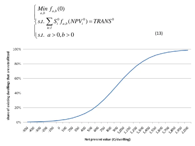
The linked hybrid model is run with two exogenous inputs: growth of the French population based on INSEE (2006), and crude oil importation price based on the American Energy Outlook 2008 (U.S. EIA, 2008)14. Domestic energy retail prices and disposable income are determined endogenously from these inputs in the static equilibrium module of IMACLIM-R. As far as Ref-IRF is concerned, population increases regularly by 13% and total income approximately doubles over the 2008-2050 period. The price index of energy consumed for space heating rises up to 18%, with fluctuations of a few percentage points (pp) due to contrasting trends for different fuel prices: the price of electricity decreases slightly, the price of natural gas increases slightly and the price of fuel oil increases markedly (figure 5).

14 _{This scenario is close to the reference scenario used during the Energy Modeling Forum 25, to which Res-IRF} participated (see Giraudet et al., 2010).

15

Figure 5: Reference energy prices

3.2 Evolution of the primary drivers of energy consumption

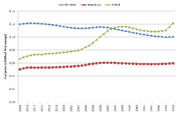
According to the business as usual scenario, energy consumption for space heating decreases by 93 TWh in existing dwellings and increases by 69 TWh in new dwellings in 2050, compared to the 254 TWh consumed in 2008. Overall, final energy consumption decreases by 10% over the 2008-2050 period, yielding an average annual growth rate of -0.3%. This evolution can be decomposed with respect to the three “primary drivers” introduced in identity 1, namely the total building stock, aggregate energy efficiency and aggregate sufficiency15. As pictured in figure 6, energy savings accruing from energy efficiency gains (conventional specific consumption decreases by an average of 1.7% per annum) are almost entirely cancelled by the rise in the building stock (by an average annual rate of 0.7%) and the fluctuating relaxation in sufficiency (the service factor increases by an average annual rate of 0.7%). Whereas the building stock and efficiency gains follow a regular trend over the long term, sufficiency adjusts to short-term energy price fluctuations. Let us examine in more detail the evolution of each of these drivers in new and existing dwellings.

15 _{Identity 1 is thus differentiated annually as δ}

16

Figure 6: Decomposition of the primary drivers of the final energy demand for space heating

Total building stock increases by 31% in quantity and by 37% in surface area over the 2008-2050 period. This projection is in line with other estimates of French building stock (Traisnel, 2001; Jacquot, 2007). Dwellings in existence in 2007 represent 62% of the total surface area in 2050 (figure 7) so retrofitting is of key importance. Note that the assumed destruction of dwellings in the lowest efficiency classes is crucial: running the model under a “no destruction” scenario (i.e. all parameters

γi equal 0) implies a net decrease in total energy consumption of 5% in 2050 compared to 2008,

instead of 10% in the business as usual scenario.

17

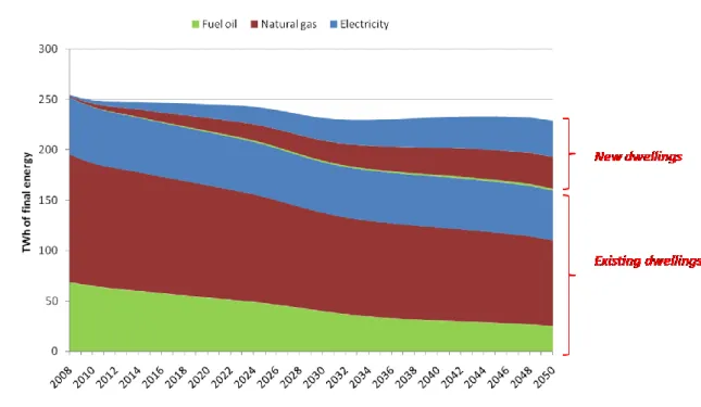
Energy efficiency gains arise from substituting efficient dwellings for inefficient ones and from fuel switching. The relative shares of energy performance categories in the cumulative stock of new buildings appear quite stable (figure 7) as construction decisions are influenced more by construction costs than by energy price variations (as reported in table 6, annex 3). The existing building stock shows the progressive disappearance of low efficiency classes G to D, together with a phased-in increase of high classes C to A (figure 8). This results from changes in the quality of retrofitting transitions, as well as in their quantity (figure 12, see below for explanations), both induced by energy price variations. As regards fuel switching, figure 9 suggests that the relative share of electricity in the consumption of existing dwellings increases16. Albeit less distinguishable, this observation holds also for new dwellings. When total building stock in 2050 is compared to 2008, the shares of electricity and natural gas in final energy consumption gain 15 pp and 1 pp, respectively, whereas fuel oil loses 15 pp. In other words, there is a general switch from fuel oil to electricity.

Figure 8: Numbers and efficiency of existing dwellings by efficiency class

16 _{Note that conventional energy consumption labeled in primary energy must be converted into final energy.} In France, the usual coefficients of primary energy units per unit of final energy are 2.58 for electricity and 1 for natural gas and fuel oil (MEEDDAT, 2008). Hence, electricity heated dwellings have de facto a lower final energy consumption than dwellings of the same efficiency class that are heated by other fuels.

18

Figure 9: Evolution of energy consumption by fuel type, in new and existing dwellings

Sufficiency relaxation is established by the rise in the total service factor, calculated, following identity 1, as the ratio of total final consumption over total conventional consumption. Figure 10 shows that this aggregate trend combines contrasting trends in new and existing dwellings; one should bear in mind that efficiency gains and increasing energy prices may have opposite effects on the service factor, as introduced in section 2.3. In existing dwellings the former prevails over the latter to yield a net augmentation in the service factor. The reverse situation occurs in new buildings where efficiency gains are insufficient to counteract the energy price increase, thus lowering the related service factor17. As a result, the service factor increases faster in the total stock than in the existing one. Indeed, as new buildings penetrate the total stock, the total factor becomes increasingly weighted by the related factor, which is declining but still higher than in existing dwellings.

17 _{Not only are the efficiency gains low, but larger gains would yield a less than proportional increase in the} service factor, as it saturates in the high efficiency domain of new construction categories (cf. figure 3).

19

Figure 10: Sufficiency effect

3.3 Reliability of the model

The reliability of the model is assessed by examining how closely it reproduces some variables of the initial situation that do not enter the calibration process, as well as how its dynamics compares to past tendencies.

Usual values Model outcomes

Annual energy expenditures for space heating

€21.2 billion in 2006, i.e. €342/inhabitant for all energy, including wood (Besson, 2008)

€18 billion in 2008, i.e.

€282/inhabitant for electricity, natural gas and fuel oil only

Total retrofitting expenditures €11.6 billion in 2006 for a total retrofitting

rate, regardless of efficiency, of 11% of the stock (Girault, 2008)

€4.8 billion in 2008 for 1% of the stock subject to the most aggressive retrofits

Average cost of the aggressive retrofits addressed by the model

€12,000 to €30,000 per dwelling, mean value of €20,000 (OPEN, 2008)

€20,000 per dwelling for transitions by at least one energy class

Direct rebound effect for space heating

Best guess ranges from 10 to 30% (Sorrell

et al., 2009)

9% in 2020 and 35% in 2050

Price elasticity of the energy demand

Long run estimates range from 0.26 to -1.89 for residential uses (Gillingham et al., 2009, table 1). They reach -0.2 in the short run in France (Besson, 2008).

-0.45 for space heating in the long run (for a 23% uniform increase in energy prices)

Trends in specific demand (m²) of final energy for space heating

-3.3% in 2005 and -2% p.a. over the 1973-2005 period (ADEME, 2008)

-2.5% in 2008 and -1% p.a. over the 2008-2040 period

20

The first three rows of table 3 show that cost estimates are fairly well reproduced by the model. The rebound effect, approximated by the growth rate of the aggregate service factor18, tends to increase but remains in the range of best guess estimates reviewed by Sorrell et al. (2009) for space heating. According to equations 9 and 14, energy prices influence both sufficiency and efficiency decisions. Following EMF13 (1996) and Boonekamp (2007), the price sensitivity of the model is assessed by changes in energy consumption due to changes in energy prices. Figure 10 compares the outcomes of two exogenous energy price scenarios: one with constant prices and one with prices increasing by 0.5% p.a. (note the limited range of values on the y-axis). The 23% price differential induces a -10% energy consumption differential in 2050 which yields a long run price elasticity of energy demand for space heating of -0.45. Again, this is in line with the usual estimates, as reviewed by Gillingham et al. (2009).

Figure 11: Sensitivity to alternative energy price scenarios

On the whole, this first run brings confidence in the model. The last row of table 3 shows that the

business as usual decrease in specific energy demand is slower than past trends. If the reliability of

the model is accepted19, this may owe more to the advanced exhaustion of the potential for aggressive retrofits, or to autonomous energy efficiency improvement measures that do not count towards an upgrade of energy class.

18 _{That is, Δ(E}

fin/Econv)/(Efin/Econv) ≈ (ΔEfin/Efin)/( ΔEconv/Econv). This can be seen as an elasticity of the energy demand to an efficiency term, which is the genuine way of defining the rebound effect (Sorrell and Dimitropoulos, 2008).

19 _{Comparing past trends to those projected by the model over the same period would have been a relevant} way to address this issue (e.g. Boonekamp, 2007). However, this cannot be achieved, since the 2007 data used to calibrate the building stock by energy performance category are the oldest available.

21

4 The potential for energy conservation in existing dwellings

This section looks at the potential for energy conservation as different barrier parameters are varied. It concentrates on the priority issue of retrofitting, the endogenous treatment of which is a distinctive feature of Res-IRF (see section 2.2.6). As depicted in figure 1, determination of the quantity of retrofits (variable Xi) is linked to determination of their quality (variable PRi,f). More

generally, this process stands at the end of the determining chain, hence it is affected by all the barriers incorporated in the model.

4.1 Determinants of technological change

The effective retrofit numbers, pictured in figure 12, follow a flat but slightly bell-shaped curve. To reveal the underlying mechanism, this curve is flanked by two dashed curves stemming from alternative scenarios: one excluding intangible costs (but assuming unchanged calibration parameters) and one assuming constant intangible costs. Both curves are unambiguously decreasing, as they are subject to the exhaustion of profitable retrofit potential. The early increase in the effective retrofitting numbers is due to information acceleration, as comparison with the frozen intangibles alternative suggests. This process enables the reference case to narrow in the long run the “absent intangibles” alternative, whereby retrofitting decisions are determined by sole financial costs: while reference retrofitting numbers reach 58% of the potential uncovered by the “absent intangibles” alternative, this ratio grows to reach 91% in 2050. Overall, the bell-shaped curve is the consequence of the countervailing effects of information acceleration, which prevails in the short and medium term, and the exhaustion of potential, which prevails in the long term.

Figure 12: Annual retrofits, in reference and in alternative scenarios

In addition to information acceleration, other factors, such as learning-by-doing and the increase in energy price, influence the general process of technological change. The price indexes of the underlying variables, namely intangible costs IC, transition costs CINV and energy prices for heating uses P, are portrayed in figure 13. The power-shaped decrease in transition costs and the logistic-shaped decrease in intangible costs appear clearly.

22

Figure 13: Evolution of retrofitting variables

The quantitative impact of each of these variables on retrofitting numbers can be assessed by freezing them, one after the other, i.e. setting parameters u and l to zero and using a constant energy price scenario. The influence of energy prices on technological change turns out to be negligible compared to other factors, as figure 14 suggests20. This may be due to the relative stability of energy price input and its regular effect on retrofitting numbers. In contrast, learning-by-doing and information acceleration are self-reinforcing processes whose magnitude inexorably increases over time. Admittedly, this is inherent in the modelling choices made in Res-IRF regarding the characterization of the processes and the parameterization of the business as usual scenario. In particular, the overwhelming effect of information acceleration relies on a vigorous logistic process, parameterized at a high information rate (see annex 1).

20 _{Figure 14 illustrates one scenario combination among six possibilities, depending on which variables are} frozen first and second. All combinations have been tested and they yield close results.

23

Figure 14: Change in annual retrofits due to freezing retrofitting variables

4.2 Sensitivity to investment parameters

The previous sensitivity analysis dealt with parameters that determine the dynamics of the model. The discount rate and the heterogeneity of preferences also determine the dynamics, but in addition, they are used to calibrate initial intangible costs (see annex 4) and retrofitting parameters (see section 2.2.6). Therefore, to illustrate their dynamic impact, alternative values are incorporated for 2010, which do not alter the calibration process. This should be interpreted as massive and durable change in investment behaviour in 2010, which is unrealistic but serves the purpose of quantifying the potential for energy conservation. For each parameter, a high and a low value is tested.

Parameter Alternative values Meaning

ν (Nu) 0 The heterogeneity is maximal and all options have the same proportion.

For instance, the proportion of any of the six possible transitions from class G is around 17%.

100 The heterogeneity is minimal and only the least cost option is chosen. For instance, the least cost transition from class G is allocated a 98%

proportion

r (DR) 7% for all decision-makers All decision-makers have a conventional private discount rate, as assumed by McKinsey&Company (2009): the landlord-tenant dilemma, as

incorporated in the model, is ignored

21% for all decision makers All decision-makers have a discount rate equal to the average one: the landlord-tenant dilemma is present but it affects indistinctively all decision-makers

24

As illustrated by figure 16, retrofitting numbers decrease with ν = 0 and r = 21% and increase with ν = 100 and r = 7%, compared to the intermediate reference scenario parameterized by ν = 8 (i.e. the least cost option gets 44%) and the heterogeneous discount rates outlined in table 2. If ν = 100, the proportion of costly transitions is lower than in the reference case (equation 5). This lowers the weighted average of transition costs, hence the net present value of retrofitting increases (equation 12), as does the retrofitting rate (equation 11). Similarly, if r = 7% for all decision-makers, the relative weight of energy operating expenditure in life cycle costs increases (equations 9 and 6), which favours the highest efficiency options compared to less efficient ones. Again, this increases the net present value of retrofitting and thus its rate. In contrast, the opposite effect occurs for alternatives ν = 0 and r = 21%.

Figure 15: Change in annual retrofits due to parameter variation

The clear impact of parameter ν on the quantity of retrofits is more ambiguous when dealing with their quality (figure 16). Compared to the ν = 100 case, the ν = 0 case emphasizes the tail distributions, e.g. the lowest efficiency class (G) but also the highest (A) in existing dwellings in 2050. Things are clearer with parameter r, as there are relatively fewer inefficient dwellings (classes G to D) and relatively more efficient ones (C to A) in the 7% case compared to the 21% case.

25

Figure 16: Change in 2050 energy class repartition due to parameter variation

Figure 17 provides conventional energy consumption (Econv) directly related to the efficiency of

existing dwellings for alternative scenarios, as percentage changes of the reference scenario. Unsurprisingly, cases that lower the retrofitting rate (ν = 0 and r = 21%) raise conventional consumption, and other cases (ν = 100, r = 7% and their combination) have the opposite effect. The picture is reversed when one considers the changes in the service factor compared to the reference scenario (figure 18), as the rebound effect retroacts over energy efficiency gains. Note that in terms of conventional energy consumption, the ability of the ν = 0 case to foster very efficient choices compensates for its dramatically depressing effect on the retrofitting rate, as its proximity to the r = 21% case suggests (figure 17) and despite a large discrepancy in the retrofitting numbers (figure 15). Hence, the trade-off between the quantity and quality of retrofits is a non-trivial issue. Note, also, that the discount rate disaggregation by decision-maker occupancy status matters, since the uniform

r = 21% case yields lower energy efficiency gains than the business as usual case in which heterogeneous discount rates have the same average value. Lastly, between the ν = 100 and r = 7% cases, the latter has a stronger impact on efficiency, which suggests that the landlord-tenant dilemma (as represented in the model) is the most significant barrier.

26

Figure 17: Change in conventional energy demand of existing dwellings due to parameter variation

Figure 18: Change in the aggregate service factor of existing dwellings due to parameter variation

4.3 Potential energy savings due to efficiency and sufficiency

By comparing the r = 7% case with the business as usual projection, the potential for energy savings accruing from both sufficiency relaxation and efficiency gains can be quantified. The potential for efficiency has been more thoroughly investigated than the potential for sufficiency (BC Hydro, 2007; Moezzi et al., 2009). From the seminal energy efficiency classification proporsed by Jaffe and Stavins (1994b, figure 1) and EMF13 (1996, figure 7 and p.24), the present assessment can be characterized as a techno-economic one, since the efficiency potential is inferred from parameter variations within a range compatible with general economic conditions. It does not quantify the maximum technical potential, as it ignores the emergence of new technologies, and fails to assume the general use of the best available technologies. This could be done by constraining transition choices to the sole most profitable option, i.e. for any initial class i, final class f = A is the only chosen option. However, this would disrupt the endogenous determination of the retrofitting rate.

27

Figure 19: Techno-economic potential for energy conservation in existing dwellings

Figure 19 shows that, compared to reference savings of 37% in existing dwellings, 10 pp could be gained if the rebound effect was totally cancelled. This could be achieved by energy taxation or information tools. In particular, giving households feedback about their energy saving has proven to be very effective, especially when peer comparison is provided (Abrahamse et al., 2005; Ek and Söderholm, 2010; Darby, 2006b; Ayres et al., 2009). Abstracting from the rebound effect, another 4 pp reduction in final consumption could be achieved through efficiency improvements. In comparison, the 13rd session of the Energy Modeling Forum reported estimates of the techno-economic potential ranging from 3 to 25%; this was established by comparing four models subject to variations in private discount rates (EMF13, 1996, figure 9). This potential could be tapped by a wide range of policies, such as information, incentives (tax and subsidy) and regulations. On the whole, 14 pp reduction could be gained or, put another way, the potential for reference savings could be enhanced by 38%, including 27% of sufficiency relaxation and 11% of efficiency improvements. In methodological terms, this is much less than the purely technical potential assessed by Baudry and Osso (2007, figure 1), according to whom tens of TWh of final energy could be saved annually in the French residential sector. In terms of policy-making, this is far from the target recently set by the French Government of reducing energy consumption in existing buildings by 38% between 2008 and 202021.

5 Conclusion

This paper exposes and evaluates the representation of household energy demand in the IMACLIM-R hybrid framework adapted to France. Res-IRF, a bottom-up module of household energy

21 _{Loi n° 2009-967 du 3 août 2009 de programmation relative à la mise en œuvre du Grenelle de}