Inverse modeling of annual atmospheric CO 2 sources and sinks: 1. Method and control inversion

HAL Id: hal-02923856

https://hal.archives-ouvertes.fr/hal-02923856

Submitted on 25 Jan 2021

HAL is a multi-disciplinary open access

archive for the deposit and dissemination of

sci-entific research documents, whether they are

pub-lished or not. The documents may come from

teaching and research institutions in France or

abroad, or from public or private research centers.

L’archive ouverte pluridisciplinaire HAL, est

destinée au dépôt et à la diffusion de documents

scientifiques de niveau recherche, publiés ou non,

émanant des établissements d’enseignement et de

recherche français ou étrangers, des laboratoires

publics ou privés.

Inverse modeling of annual atmospheric CO 2 sources

and sinks: 1. Method and control inversion

P. Bousquet, P. Ciais, P. Peylin, M. Ramonet, P. Monfray

To cite this version:

P. Bousquet, P. Ciais, P. Peylin, M. Ramonet, P. Monfray. Inverse modeling of annual atmospheric

CO 2 sources and sinks: 1. Method and control inversion. Journal of Geophysical Research:

At-mospheres, American Geophysical Union, 1999, 104 (D21), pp.26161-26178. �10.1029/1999JD900342�.

�hal-02923856�

JOURNAL OF GEOPHYSICAL RESEARCH, VOL. 104, NO. D21, PAGES 26,161-26,178, NOVEMBER 20, 1999

Inverse modeling of annual atmospheric C02 sources and sinks

1. Method

and control inversion

P. Bousquet,

• P. Ciais, P. Peylin, M. Ramonet,

and P. Monfray

Laboratoire des Sciences du Climat et de l'Environnement, Gif sur Yvette, France

Abstract. A primary goal of developing

the CO2 atmospheric

measurement

network is to better

characterize

the sources

and sinks of atmospheric

CO2. Atmospheric

transport

models can be

used to interpret

atmospheric

measurements

in terms of surface

fluxes using inverse

methodology.

In this paper we present

a three-dimensional

(3-D) inversion

of CO2

measurements

in order to infer annual sources

and sinks of CO2 at a continental

scale (continents

and ocean

basins)

for a climatological

year representing

the 1985-1995 period. Solving this

inverse

problem

requires

(1) a data space

representing

monthly CO2 measurements,

here at

77 sites

(surface,

ships,

planes),

(2) a flux space

describing

a priori fluxes between

carbon

reservoirs,

and (3) a 3-D transport

model linking the flux space

to the data space. Knowledge

of

these three elements,

together

with their associated

errors,

allows one to reduce the uncertainties

of the CO2 sources

and sinks.

In the 1985-1995 period, for our control

inversion,

the global

continental

sink is found

to be 2.7+ 1.5 Gt C yr i for an optimized

deforestation

source

of

1.4+0.6

Gt C yr 1 , yielding

a net land uptake

of 1.3+

1.6 Gt C yr 1 (fossil

fuel removed).

The

continental

partition

of this budget

is (in units

of Gt C yrl): Arctic

+0.2+0.3,

North America

-0.5+0.6, Europe -0.3+0.8, north Asia -1.5+0.7, tropics

(except

Asia) +0.3+0.9, tropical Asia

+0.8+0.4, and Southern

Hemisphere

-0.1 +0.3. The inferred

partition

for the controversial

Northern Hemisphere

CO2 sink reveals that a major sink is located

over the north Asia

continent.

For oceans

we find a net global

sink of 1.5+0.5

Gt C yr 1 with the following

partition

(in units

of Gt C yr•): North Pacific

-0.3-½0.2,

North Atlantic

-0.8+0.3, equator

+0.6+0.2,

1. Introduction

CO 2 is the second

most important

greenhouse

gas in the

Earth's atmosphere, after water vapor. Its concentration has increased by 30% over the past 200 years in response to industrialization and to land use changes [Intergovernmental Panel on Climate Change (IPCC), 1995]. The industrial source is known with a relatively good level of accuracy [Andres et al., 1993] while the land use induced source is more difficult to estimate [Houghton, 1997]. From the observed CO2 growth rate in the atmosphere, which is documented at many observing sites around the world [Conway et al., 1994], we know that on average, only about half of the human-induced emissions end up being stored in the atmosphere [IPCC, 1995]. The other half is currently reabsorbed by natural resevoirs, oceans, and land biosphere.

If we are to make reliable predictions of future CO2 levels, we need not only to make projections of the human-induced source but also to estimate the response of the oceans and of the land ecosystems to rising CO 2. To do so, it is of primary importance to establish a precise diagnostic of today's carbon budget. This requires not only estimation of global CO2 uptake partitioning

I Also at Universitfi de Versailles Saint Quentin en Yvelines, Versailles, France

Copyright 1999 by the American Geophysical Union. Paper number 1999JD900342.

0148-0227/99/1999JD900342509.00

between oceans and continents, but also its space and time distribution. Furthermore, large positive and negative anomalies of the CO 2 growth rate, correlated or lag correlated with the climate variability, indicate that we need long time series of observations to remove year-to-year variability from the long- term sources and sinks activity [Conway et al., 1994 ; Keeling et al., 1996a].

Direct atmospheric observations can be used to infer large- scale patterns of the CO 2 surface fluxes. Small, but accurately measured, gradients in CO 2 concentration between different points on the globe relate to the sources distribution and to the atmospheric transport [Keeling et al., 1989; Tans et al., 1990]. In this study we use the monthly mean CO 2 measurements made over the past 15 years at 77 sites worldwide with: the Global Atmosphere Watch (GAW) from World Meteorological Organization (WMO), the Climate Monitoring and Diagnostic Laboratory (CMDL) from National Oceanic and Atmospheric Administration (NOAA/USA), the Laboratoire des Sciences du Climat et de l'Environnement (LSCE) from Institut Pierre Simon Laplace (IPSL/France), the CSIRO Division of Atmospheric Reasearch (DAR/Australia), the Atmospheric Environment Service (AES/Canada), and Japan networks. These data are aggregated into the GLOBALVIEW database [Cooperative Atmospheric Data Integration Project: Carbon Dioxide, 1997; Masarie and Tans, 1995] which is a comprehensive database of CO 2 concentrations at more than 70 sites, smoothed, interpolated, and extrapolated on a weekly time step over the 1980-1997 period. They are used together with a global model of the atmospheric transport to deduce the CO2 sources and sinks annual magnitude over large areas at the surface of Earth. We use a Bayeasian inverse procedure in order to determine the annual

26,162 BOUSQUET ET AL.: METHOD OF INVERSE MODELING OF CO 2

magnitude of sources and sinks that gives model CO2 in best agreement with the entire data set of atmospheric measurements [Tarantola, 1987; Enting et al., 1993].

We consider several spatial scales in this paper. The spatial scale used for inverse calculation is the regional scale (1000-3000 km). Optimized fluxes are then aggregated at the scale of large ocean basins and continental areas (3000-10 000 km). This spatial scale will be hereinafter referred to as the continental and ocean basins scale. Optimized fluxes are also analyzed for three major latitude bands (15øN-90øN, tropics, 15øS-90øS) and at global scale. We optimize annual mean CO 2 sources and sinks, but we use montly a priori flux estimates and monthly atmospheric observations. Furthermore, we only consider one climatological year of atmospheric observations, that is, the average of the 1985-1995 period.

Several inverse calculations have been performed since the early 1990s, mostly relating meridional gradients in CO2 (and isotopes) to the latitudinal distribution of the fluxes [Bousquet et al., 1996; Ciais et al. , 1995b; Enting and Mansbridge, 1991 ]. The inverse method presented here, based on the ideas of Enting et al. [1993] and Tarantola [1987], uses gradients among stations both in latitude and longitude to infer fluxes over different regions of the globe. It has the advantage of estimating the errors on the inferred sources and thus providing some degree of confidence on the results. It has the disadvantage of depending to a certain extent, on some prior knowledge of the problem, such as prior estimates and uncertainties of the sources strength or patterns in their geographical distribution. Thus, we need to verify carefully that the inferred fluxes and their numerical stability are mostly constrained by the atmospheric observations through the atmospheric transport, and not by a priori information. In the following, we describe the method that is used to infer

the

CO2

budget

(section

2). Also,

measurements

of 813C

in CO2

can be used to separate ocean uptake from land uptake within a given band of latitude [Ciais et al., 1995a]. This arises from the

fact

that

13

C fractionations

during

photosynthetic

carbon

uptake

and

air-sea

exchange

processes

are

different.

However,

no 813C

data are included in our control inversion. The specific

methodology

to include

813C

data

as additional

constraints

into

the inversion is fully described by Bousquet et al. (this issue, the appendix). We then detail the components that are necessary for the inverse procedure: the model of atmospheric transport, the atmopheric data, and the "prior" flux scenario (section 3). We discuss the results for the inferred annual source strengths of our control inversion (hereinafter noted So) at global scale in section 4 and at continental and ocean basins scale in section 5. Special attention is given to the existence of CO,_ gradients between marine sites and sites under a more continental influence and to how they relate to the partitioning of the CO 2 fluxes between

ocean and land.

2. Method

2.1. Cost Function

Bayesian time-independent inversion is a technique that is used to optimize surface fluxes of atmospheric trace gases against a set of atmospheric data, given a priori knowledge of surface fluxes with standard deviations [Enting et al., 1995, 1993; Hein et al., 1997]. This technique and the statistics related to it are fully described by Tarantola and Vallette [1982], Tarantola [1987], and Enting et al. [1993]. Briefly, we subdivide the surface fluxes into individual sources, each corresponding to a region and/or a specific type of emission (e.g., fossil fuel

combustion and photosynthesis). Each individual source has a given spatial pattern, intra-annual variations, and an overall

source

strength

mj (with

standard

deviation)

in gigatons

of carbon

per

year

(Gt C yr-1).

Annual

source

strengths

mj are

the

parameters we optimize in order to match the modeled CO2 concentrations with the observed ones. Monthly averaged observations of atmospheric CO2 at 70 monitoring sites were extracted from GLOBALVIEW-CO 2 extended database [Cooperative Atmospheric Data Integration Project: Carbon Dioxide, 1997; Masarie and Tans, 1995] for the period 1985- 1995, which is our reference period. The seven other sites come from aircraft mesaurements over Japan and Tasmania at different altitudes. All data are used to build a climatological database of CO 2 concentrations (represented by a vector dobs). Control inversion S O is thus a steady state experiment performed only with CO2 data. For each regional source we normalize the flux to

1 Gt C yr

-1 (normalized

source

base

function).

Then we

determine

a vector

mp containing

a priori knowledge

of annual

source strengths for all sources and all regions (see section 3). Source base functions are prescribed to an atmospheric transport model (named g) which produces the normalized model responses at all monitoring sites for each regional flux component d-g(m). This step is called the direct problem. The inverse problem, that is, deducing optimized sources and sinks from atmospheric measurements, is overconstrained as the dimension of d is greater than the dimension of m. For the standard inversion, we use a vector d of 77x12=924 elements and a vector m of 46 individual sources to describe CO2 fluxes. Finally, the error due to the atmospheric transport model is not considered mathematically in this paper but will be considered as part of the sensivity study [Bousquet et al., this issue]. Assuming that all uncertainties are Gaussian and uncorrelated spatially and temporally, solving the inverse problem to infer optimized sources and sinks means to minimize the cost function S(m) given by Tarantola [ 1987]:

1

{[g(m)

-dobs]

t Cc/-l[g(m)

-dobs]

S(m)

= •

+(m-mp)

tCm-l(m-mp)}

(1)

here Cd is the diagonal covariance matrix for atmospheric data and Cm is the diagonal covariance matrix for a priori fluxes. The expression of g(m) depends on the tracer studied and on the

model used.

2.2. Solution of the Inverse Problem

Atmospheric transport of an inert tracer like CO2 is a linear operator. It means that CO 2 concentration at a given point of the

atmosphere

( Zco,) can

be expressed

as a linear

combination

of

the modeled

resfionses,

•;/, of the normalized

source

base

functions,

F•, as

/v.,

ZCO,

= Ztn/•:/ with

- Pj

(2)

J=l

where

N s is the number

of source

base

functions,

m

s represents

the annual source strength of the jth source. In a matrix form we can write vector d of model outputs as

d=Gm (3)

where

G ij is the contribution

of source

j to the concentration

at

BOUSQUET

ET AL.: METHOD

OF INVERSE

MODELING

OF CO2

26,163

corresponding

to a global

CO 2 "offset"

which is optimized

at the

same time as the source strengths. This global "offset" represents the average CO2 concentration in the atmosphere in the absence of any sources and sinks. G has additional rows which insure global mass conservation and allow specific constraints on a group of individual sources (see section 3).

S(m)

=

•[(G

m-

dobs)t

Ca-l(G

m-rob

s)

+(m-my)

t Cm-l(m-

my)

]

(4)

From Tarantola [1987] we obtain the maximum likelihood vector m which corresponds to the optimized annual sources and sinks as

/ •=mp

+(GtC•G+C•n

! GtC•(dobs

-G m

e) (5)

\m/

and the a posteriori covariance matrixes C'rn and C' d for fluxes and atmospheric data, respectively:

' (6)

= c;c;.c;'

(7)

The

matrix

₍

G

tC•G+ • -•

_{C•n) is}

_inverted

_using

_either

_singular

value decomposition (SVD) or Choleski decomposition

techniques

(Interactive

Data Language

(IDL) numerical

package,

adapted from Press, et al. [1987]).

3. Required Components

of the Inversion

As we have seen in section 2, continental synthesis inversion requires three sets of information: a set of atmospheric observations to be fitted, a set of source base functions, and a set of calculated model responses, the latter being computed from a global model of atmospheric transport.

3.1. Atmospheric Data

We use a subset of the GLOBALVIEW-CO2 database [Cooperative Atmospheric Data Integration Project.' Carbon Dioxide, 1997; Masarie and Tans, 1995], plus vertical profiles at a few selected locations. GLOBALVIEW-CO 2 is a data set of CO2 concentrations where the time series of individual discrete flasks or continuous record is smoothed in the time domain. Gaps in the data are filled using an extension scheme as described by Masarie and Tans [1995] and Thoning et al. [1989]. Thus

GLOBALVIEW-CO

2 provides smoothed continuous

CO 2

records on a weekly time step at more than 80 monitoring sites between 1980 and 1995. As many new measurement sites

appeared

between

1980 and 1985,

we discard

data for this period

to focus on the 1985-1995 period, which is our reference period in this paper. This choice is to limit the influence of changes in the number of sites of the network on the solution of the

inversion.

It is important to note that GLOBALVIEW-CO2 employs data from different networks, although NOAA CMDL data are by far the most extensive. Thus possible calibration offsets or errors between networks may translate into CO 2 differences between stations. Nevertheless, the data included in GLOBALVIEW-CO 2 are part of the WMO GAW program, and numerous intercomparisons between the different groups have shown that

the CO 2 offsets among the main contributing networks do not exceed 0.5 ppmv.

Two time series of aircraft measurements are also used in

addition to the GLOBALVIEW-CO 2 data. Above Sendai (Japan, 140øE, 38øN), data from 1982 to 1994 are grouped into altitude bands: 0-2 km, 2-4 km, 4-8 km, and 8 km-tropopause [Tanaka et al., 1987]. Above Cape Grim (Tasmania, 140øE, 40øS), we have grouped the 1974-1991 measurements in two levels: 3 km and 6 km [Pearman and Beardsmore, 1984; Monfray et al., 1996; Pak et al., 1997]. Aircraft measurements are smoothed within the time domain using exactly the same pro,cedure as for surface data

[Thoning

et al., 1989]. However,

aircraft

data are not

extrapolated beyond the measured time domain. The map of all measurement sites is plotted on Figure 1: most of the sites are located in the Northern Hemisphere (57 of 77), and most stations are located in the marine boundary layer. For each site we calculate 12 monthly values that are averages representing the 1985-1995 period. We also compute 12 monthly standard deviations for all sites. The procedure to calculate these monthly averages is detailed in Appendix A.

3.2. A Priori Flux Scenario

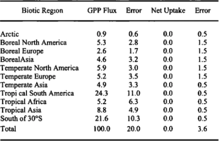
3.2.1. Fluxes. For each type of source involved in the CO2 budget we establish a global map of a priori fluxes on a monthly basis. The sources which are considered in this paper are listed and briefly summarized in Table 1. They correspond to fossil fuel emissions (FOS), land use changes (DEF), gross primary production over lands (GPP), total respiration over lands (RES), land net uptake (BIO_UPT), and net ocean fluxes (OCE). Each source is further subdivided into several components corresponding to different regions (source regions) which

determines the source base functions. Note that for land areas the number of source base functions is 3 times the number of source

regions because we have three spatial and temporal patterns representing the continental exchanges (GPP, RES, and BIO_UPT). We choose 3xl 1 regions to account for continental fluxes, eight regions to account for ocean fluxes (see Figure 2). Moreover, three tropical regions are used for land use changes (tropical America, tropical Africa, and tropical Asia), and one global region is used for fossil fuel emissions. These geographical patterns determine 37 source base functions for continental processes and eight source base functions for oceanic ones. For further details on the a priori scenario, please refer to Appendix B. One should notice that for land uptake (BIO_UPT) we use the spatial pattern from Friedlingstein et al. [1995].

However,

we set the a priori

value

of BIO_UPT

to 0.0 Gt C yr l

for each

region

with large

standard

deviations

of 1.5 Gt C yr 1 for

nontropical

regions

and 0.5 Gt C yr 1 for tropical regions.

3.2.2. Errors. For each source base function a standard deviation associated to the annual flux is determined either as a

percentage of the flux (gross fluxes) or as an arbitrary large value. For gross fluxes (GPP and RES) we set the a priori

standard

deviation

rs

j proportional

the flux itself

(20%). Then

we compute

the

error

rs

j,/, associated

to each

region

k according

nb_comp

2= 2

rs./ Z rs.i,k

(8)

k=l

For atmospheric

growth

rate,

fossil

fuel emissions

and land

use

change

we take

the

IPCC [1995]

estimates

of O'j (Table

1). For

ocean

and land uptake,

which are the most

uncertain

net fluxes,

26,164 BOUSQUET ET AL.: METHOD OF INVERSE MODELING OF CO 2

la.i

100øE 140øE 180 ø 140øW 100øW 60øW 20"W 20øE 60øE

90øN

'

'

'

'

' A•-[ ...

MBC

•••_.•..•

ZEP

"' CBA

NWR •

AZR ••

n=c

•-''

SHU

50ON

i

/

100øE 140øE 180 ø 140øW 100øW 60øW 20"W 20øE 60øE 100øE LONGITUDE

Figure

1. Atmospheric

network

used

for the inverse

calculation

S

0. Dots

represent

ground

measurements

made

by

different

research

groups

around

the

world. Lines

represent

ship

data.

Small

planes

indicates

vertical

profiles

used

Iceland;

CBA,

Cold

Bay;

WES,

Westerland;

MHT,

Mace

Head;

SHM,

Shemya

Island;

CSJ,

Cape

S

t James;

OPW,

Olympic

Peninsula;

SCH, Schauinsland;

CMO, Cape

Meares;

CIM, Monte Cimone;

SBL, Sable

Island;

NWR,

Niwot Ridge;

UTA, Utah;

RYO, Ryori;

AZR, Terceira

Island;

TAP, Tae-ahn

Peninsula;

QPC, Qinghai

Province;

KSN, Korean

station;

BMW, Bermuda

West; IZO, Tenerife;

MID, Sand

Island;

KEY, Key Biscayne;

KUM, Cape

Kumukahi;

MLO, Mauna

Loa;

AVI, S

t Croix;

GMI, Guam

Island;

RPB,

Ragged

Point;

CHR, Christmas

Island;

SEY, Seychelles;

ASC, Ascension

Island;

SMO, American

Samoa;

AMS, Amsterdan

Island;

CGO, Cape

Grim;

BHD, Baring

Head;

CRZ, Crozet

Island;

MAQ, Maquarie;

PSA, Palmer

Station;

MAW, Mawson;

SYO, Syowa;

HBA, Halley Bay; SPO, South

Pole;

P01 to P16, Pacific

cruises;

C01 to C07, China Sea cruises;

S02 to S06,

Aircraft measurements above Japan; CG4 and CG6, Aircraft measurements above Tasmania. we assign arbitrary large regional errors so that global errors are

of ñ3.0 Gt C yr ] and ñ3.6 Gt C yr • respectively

. Large errors

limit the bias introduced by the use of a priori flux values on the

result of the inversion.

3.3. Atmospheric Transport

The calculations of the modeled concentrations produced by source base functions are performed with the TM2 model

[Heimann,

1995] using 9 sigma vertical levels at a 7.5øx7.5

ø

horizontal resolution [Ramonet, 1994]. Analyzed meteorological data for the year 1990 [European Center for Medium-Range Weather Forecast (ECMWF), 1994] are used both for horizontal and vertical transport (convection and vertical diffusion). The

time step of the meteorological

fields is 12 hours,

whereas

the

model time step is 3 hours. Advection is calculated using the Russel and Lerner [1981] slope scheme. In each grid box and at Table 1. Global Processes, Annual Fluxes and Errors Involved in Atmospheric CO2 Cycle

Process Flux and Errors Seasonality References

Atmospheric increase 3.1 + 0.1 - Conway et al. [1994] Anthropic perturbation 7.5 + 1.1 - IPCC [ 1995] Fossil fuels 5.9 + 0.3 yes Andres et al. [ 1997]

Rotty [ 1987] Deforestation 1.6 + 1.0 yes Houghton [ 1997] Biotic fluxes - 1.8+ 1.6 - IPCC, [ 1995] GPP - 100 + 20 yes Denning et al. [ 1996],

Sellers et al. [ 1996a,b, 1986] Total respiration 100 + 20 yes Denning et al. [ 1996] biotic uptake - 1.8+ 1.6 yes Friedlingstein et al. [ 1995] Oceanic fluxes -2.0 + 0.8 - IPCC [ 1995]

oceanic uptake plus seaonality - 1.2 + 0.8 yes Takahashi et al. [ 1997]

•3OUSQUET

ET AL.:

METHOD

OF INVERSE

MODELING

OF CO2

-3O

-180 -120 -60 0 60 120 180

Longitude

Figure 2. Oceanic (o 1 to o 8) and continental (b 1 to b 11) regions used by the control inversion So: b 1, Arctic (north of 65øN); b2, Boreal North America; b3, Boreal Europe; b4, Boreal Asia; bS, Temperate North America; b6, Temperate Europe; b7, temperate Asia; b8, tropical South America; b9, tropical Africa; b 10, tropical Asia; b l 1, southern nontropical hemisphere; and o 1, north of 65øN; o 2, North Pacific; o 3, far North Atlantic; o 4, North Atlantic; o 5, equatorial oceans, o 6, subantarctic and subtropical oceans; o 7, austral ocean (south of 50øS).

26,165

each time step this scheme calculates the concentrations as well as the gradient of concentration in the three physical directions (longitude/latitude/altitude). Turbulent vertical transport is calculated by stability-dependent vertical diffusion using the parametrisation of Louis [ 1979]. Convection is represented using Tiedtke's [1989] scheme, which is based on humidity convergence in the low atmosphere. As explained by Heirharm [1995], there is no explicit horizontal diffusion in

this version of the model.

The TM2 model is part of the range of models in the TRANSCOM intercomparison experiment (Special project of the IGBP Global Analysis, Interpretation, and Modelling (GAIM) Task Force, http://gaim.sr.unh.edu/Projects/TRANSCOM/) that do not present a strong "rectifier" effect of concentrations above continents [Law et al., 1996; Denning et al., 1997a]. It has the advantage of fast computational performances which allows the

use of many source base functions. The TRANSCOM I

experiment

revealed

that some models

could produce

large

positive CO2 zonal mean profiles (south to north) when prescribed with a purely seasonal biotic source (no annual net flux). Such an effect is caused by both the accumulation of respired CO 2 during winter over Northern Hemisphere continents and the dilution of the uptake imposed by photosynthesis during

,, ,,

summer. This so called rectifier effect of concentrations is documented by Denning et al. [1995]. It i•ntroduces large uncertainties associated to vertical transport especially over continents [Denning et al., 1997a]. The exact intensity of this effect still remains to be quantified. For instance, recent tests have shown that the Colorado State University (CSU) model probably greatly overestimates this effect [Denning et al.,

1997b]. The TM2 model does not produce a significant rectifier effect above continents due to its coarse vertical resolution near

the surface (0.4, 1.2, and 3.6 km for the center of the three lowest grid boxes, re,.spectively). At the opposite, the TM3 model introduces a rectifier effect of almost 2 ppmv in the biospheric TRANSCOM I experiment [Law et al., 1996]. The TM3 model is

a new version of TM2 model with a 4øx5 ø horizontal resolution

and 19 vertical levels. It was developed by M. Helmann at Max

Planck Institute. Using both TM2 and TM3, Bousquet et al. (this issue, section 4) analyze the influence of atmospheric transport

on the results of the inversion.

Each source base fu..nction consists of 12 monthly flux fields (with spatial patterns). Each base function has been run for 4 years in the atmospheric transport model to achieve steady state [Helmann et al., 1989]. Only 1 year of atmospheric forcing has been used repeatedly during the 4 years of simulation (ECMWF, year 1990). The last year of si..mulation is used to calculate monthly modeled CO2 concentrations at each site. Instead of

taking the average

CO2 concentration

in the grid box, we have

sampled the model outputs of the fourth year of simulation at the exact position of the monitoring sites. The concentration at the

location

of the monitoring

sites is taken precisely

using the

concentrations slopes given by the advection scheme. Moreover, in order to account (partly) for data selection we have extracted

the concentrations of the closest oceanic model box for two coastal monitoring sites, Bermuda (BMW) and Cape Grim (CGO). No other mode,1 output selection has bee.n pe,rformed.

3.4. Additional Constraints

Additional independent constraints are introduced as additional rows to the G ma.trix. These constraints are of three kinds. First, we use the global trends which are determined with

excellent

precision

from

atmospheric

network,

1.4

+0.1 Gt C yr l

and

ocean

uptakes:

B!O_UPT

with -1.8 •:1.5

Gt C yr I and

OCE

with -2.0 +0.8 Gt C yr •. These constraints

correspond

to

independent information that we can use to improve global constraints on fluxes [IPCC, 1995]. Variances associated with these constraints are smaller than the sum of .regional variances as

26,166

BOUSQUET

ET AL.: METHOD OF INVERSE MODELING OF CO 2

4. Optimized Global and Hemispheric Net Fluxes

The optimized time series at eight monitoring sites are shown on Figure 3 together with the apriori time series and observations. The fit of monthly means is improved by the inverse procedure and is satisfying for most sites. However, the inversion performs better for nontropical sites. There are only a few sites where the fit to CO2 signal is poorly reproduced (BAL, SHM, CIM, TAP, C07, UUM, P11) either in seasonal cycle or annual mean. On Figure 3 station C07 (China Sea boat) shows the worse fit to the observations that we obtain. Atmospheric

tracer transport is difficult to reproduce in the tropics because a large part of the tracer is injected higher in altitude by convective mixing and vertical diffusion depending on the position of the Intertropical Convergence Zone (ITCZ). Especially, part of the CO2 emitted over the Northern Hemisphere and traveling south is brought aloft at the ITCZ and diluted higher up. The vertical processes involved depend greatly on the parametrization used [Law et al., 1996; Mahowald et al., 1995]. Also we know that some continental sites where CO2 concentrations can depend strongly on local effects are not well represented (some months) by the coarse resolution of the transport model used (e.g., BAL or TAP). Thus, even if the fit is correct, there is a risk that our

365

..• 360

a- 355

350

345

ALT laf'82.40 Ion'-62.50

'•\ I I/ • '

•\\ l/.

!

TAP laf:56.70 Ion'126.10

_'_

c• 352

KUM laf'19.50 Ion'-154.80

J F M A M J J A S 0 N D months 357 356

355

COO laf:-40.70 Ion'144.70

J F M A M J J A S 0 N D months 354 353 352 351 35O 349

SPO laf:-90.00 Ion'-180.00

ß i i i i i I i i i i

J F M A M J J A S 0 N D months

Figure 3. Modeled

and

observed

CO2 concentrations

for 8 of the 77 monitoring

sites

used

in control

inversion

So.

Dots stand

for atmospheric

data

(one climatological

year of observations

averaging

the 1985-1995

period).

Dashed

line is for the a priori modeled

concentrations.

Solid line is for the optimized

model

concentrations.

BOUSQUET ET AL.' METHOD OF INVERSE MODELING OF CO2 26,167 360 558 .556

,354

Latitude

Gradient

Model A PosterJori

---Model

A Priori

ß Observations

!•, ;,

'.•i•_'

I!!11b•.•t

• •' '

350

f , ,

Figure 4. North-to-south gradient. Modeled and observed CO2 annual concentrations for the 77 monitoring sites used in the control inversion S O . Dots stand for atmospheric data (one climatological year of observations averaging the 1985-1995 period. Dashed line is for the a priori modeled concentrations. Solid line is for the optimized model concentrations.

inverse method converts model bias in term of changes in the

flux estimates.

Figure 4 presents north to south annual concentrations at monitoring sites. The inversion reduces zonal north-to-south annual gradient and matches rather well annual concentrations at most of the sites. One can notice a systematic offset of the

concentrations at CGO station that will be discussed in section

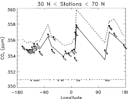
5.1. Figure 5 plots the longitudinal gradient of concentration for

sea level stations located within 35øN-65øN latitude band. This

represents 24 stations: seven in North Pacific Ocean, five in north America, five in North Atlantic Ocean, three in Europe, and four in Asia. One should note that large CO2 gradients between continental and marine sites are globally reproduced by the source adjustment in this latitude band. The two deeps of the Pacific and Atlantic Oceans are very well matched. The inverse procedure reproduces the high level of CO2 concentrations found over continents (KSN and TAP) except for the Baltic Sea site (BAL). On the west part of the North Atlantic, optimized concentration is averaged between Bermuda island (BMW) and Sable island (SBL) and does not completely reach the high CO2 level observed at SBL. The two sites of Monte Cimone (CIM) and Niwot Ridge (NWR) are not completely resolved by the inverse procedure. This result can be explained by the location of these sites at 2165 m and 3475 m respectively above sea level. For such sites at high altitude the coarse resolution of the model on the vertical direction makes it difficult to represent them properly.

4.2. Global and Latitudinal Totals

Net CO2 fluxes inferred by control inversion So at the global scale and at the hemispheric scale for three latitudinal bands are given in Table 2. Please note that (1) fossil fuel emissions have been removed from all continental fluxes presented in the

following

and

(2) some

+0.1

Gt C yr-1

discrepancies

occur

in our

360 358 356 o 354 352 - 350 -180 30 N < Stations < 70 N

' '

,'.',

',

',

Longitude

Figure 5. West-to-east gradient. Modeled and observed CO 2 annual concentrations for monitoring sites located between 30øN and 70øN. Dots stand for annual means of atmospheric data (one climatological year of observations averaging the 1985-1995 period. Dashed line is for the a priori modeled concentrations. Solid line is for the optimized model concentrations.

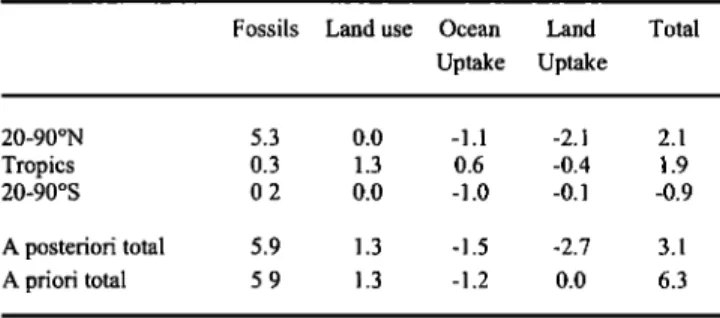
26,168 BOUSQUET ET AL.' METHOD OF INVERSE MODELING OF CO 2 Table 2. Global Results of the Standard Inversion So

Fossils Land use Ocean Land

Uptake Uptake Total 20-90øN 5.3 0.0 -1.1 -2.1 2.1 Tropics 0.3 1.3 0.6 -0.4 1.9 20-90øS 0.2 0.0 -1.0 -0.1 -0.9 A posteriori total 5.9 1.3 -1.5 -2.7 3.1 A priori total 5.9 1.3 -1.2 0.0 6.3

In Gt C yr-1

tables due to round off errors. At a global scale we obtain a

global

biospheric

sink

of 2.7+1.5

Gt C yr

-1 (1.4

Gt C yr

-1 for

total land uptake with deforestation added) and an ocean sink of

1.5+0.5

Gt C yr-

1 for

the

1985-1995

period.

Note

that

the

global

calculated flux partition between oceans and continents remains within error bars of the IPCC budget (the biospheric sink is

higher

than

IPCC

by 0.9 Gt C yr-1 and

the

ocean

sink

is smaller

by 0.5 Gt C yr-1). One

should

note,

however,

that

the IPCC

budget is set for the 1980-1989 period and not for 1985-1995

decade as in this work. The rather small ocean sink is consistent

with

the range

of 1.5-2.2

Gt C yr-1 of the

recent

ocean

model

intercomparisons conduced in the ocean Carbon-Cycle model IntercomparisonProject (OCMIP, IGBP/GAIM project, http://www.ipsl.jussieu.fr/OCMIP/, Orr et al., [ 1996]).

We find that 80% of the biospheric sink is located at the mid

to high

latitudes

of the Northern

Hemisphere

(2.1 Gt C yr-1),

against 15% in the tropics and only 5% in the Southern Hemisphere. Considering the net biospheric flux (BIO_UPT+DEF), we find that the tropical biosphere is a net

source

of 1.0

Gt

C yr

-1.

The

ocean

sink

is equally

[•artitioned

between the Northern Hemisphere (-1.1 Gt C yr -•) and the

Southern

Hemisphere

(-1.0

Gt C yr-1),

with

an

equatorial

source

of 0.6

Gt C yr

-1. If we take

into

account

all the components

(including fossil fuels), one can see that mid and high latitudes of

the

Northern

Hemisphere

are

a net

source

of 2.1 Gt C yr-1 and

tropics

are

a net source

of 1.7

Gt C yr-1 whereas

the Southern

Hemisphere

has

a net sink

of 0.9 Gt C yr

-1. In the following,

fossil fuel emissions are always removed from land flux values. Concerning the reduction of a posteriori flux uncertainties, Table 3 shows that ocean flux uncertainties are globally more reduced than continental flux uncertainties (see last column of Table 3). This result can be explained by the fact that we use only eight source base functions to represent the ocean in the inversion and also because the atmospheric network contains mainly measurement sites representative of the marine boundary layer which therefore constrain better the fluxes over oceanic regions.

4.3. Comparison With Other Studies

Previous studies have estimated the CO 2 surface fluxes for the 1980s and the 1990s [Bousquet et al., 1996; Ciais et al., 1995b; Enting and Mansbridge, 1991; Enting et al., 1995; Keeling et al., 1989; Raynet et al., 1997; Tans et al., 1990]. These studies cover different time periods and use mainly three types of constraints to infer net fluxes. Table 4 presents their results as well as constraints and covered periods. First, Keeling et al. [1989] take

historical

CO2 and

•513

C atmospheric

data

to constrain

a box

model based on the work by Oeschger et al. [1975]. Second,

Tans et al. [1990] have used two different constraints: North-to- south zonal mean CO2 gradient is the primary constraint and air- sea ApCO 2 data are the secondary constraint. Third, with the development of three-dimensional transport models at the beginning of the 1990s, concentration differences between monitoring sites have been widely used by several authors to

constrain

CO2 fluxes

[Enting

et al., 1995;

Kaminski

et al.,

1997;

Raynet

et al., 1997].

All these works cover different periods of time. For the 1980s, differences between the scenarios of Keeling et al. [1989] and

Tans

et al. [1990]

have

been

already

analyzed

[Tans

et al.,

1995].

Primary

constraints

are not the same,

but above

all,

ApCO2 data used by Tans et al. [1990] are not compatible with a strong ocean uptake. For 1992-1993, Ciais et al. [1995b] find a strong sink in the continental biosphere of the mid-Northern

Hemisphere

latitudes,

using

both

CO

2 and

•513C

atmospheric

data

the

3-D model

contribute

to both

a 0.5 Gt C yr-1

reduction

of the

equatorial source and of the global mid-latitude sink (ocean plus continents). However, the main sources and sinks regions inferred by Ciais et al. for early 1990s are confirmed by the work of Bousquet et al. 1996].

On average for the 1980s and the 1990s, the work of Raynet et al. [1997], based on the work ofEnting et al. [1995], is the most comparable work to our control inversion S O . The main differences between the two approaches are the transport model

Table 3. Regional Results of the Standard Inversion So

A Posteriori A Priori Error

Continents -1,3 + 1,6 1.6' + 4,0 60 20øN-90øN -2,2 + 1,2 0,0 + 3,7 68 Arctic 0,2 + 0,3 0,0 + 0,5 50 North America -0,5 + 0,6 0,0 + 2,0 70 Europe -0,3 + 0,8 0,0 + 2,0 60 Asia -1,5 + 0,7 0,0 + 2,0 65 Tropics* 1,0 + 1,0 1.6' + 1,5 33 South America 0,1 + 0,7 0,6 + 0,9 22 Africa 0,2 + 0,6 0,4 + 0,9 33 Asia 0,8 + 0,4 0,6 + 0,9 56 20øS-90øS -0,1 + 0,3 0,0 + 0,9 68 Oceans -1,5 + 0,5 -1,2 + 3,0 85 20øN-90øN -1,1 + 0,3 -1,0 + 0,9 61 North Pacific -0,3 + 0,2 -0,4 + 1,0 84 North Ptlantic -0,8 + 0,3 -0,6 + 1,4 79 Tropics* 0,6 + 0,2 0,8 + 1,5 90 20øS-90øS -1,0 + 0,3 -1,1 + 2,1 87 20-50øS oceans -0,9 + 0,3 -0,8 + 1,5 83 Austral ocean -0,1 + 0,1 -0,3 + 1,5 93

In Gt C yr

-1 .

* Land use and land uptake have been added in the tropics for both a priori fluxes and a posteriori fluxes. A priori land uptake is chosen to be

0.0+4.0Gt

C yr

-1 in order

not to introduce

a bias

in the optimized

solution.

A priori

deforestation

is 1.6+0.8

Gt C yr

-1 . Error

represents

the

BOUSQUET ET AL.: METHOD OF INVERSE MODELING OF CO2 26,169 Table 4. Comparison of S o With Other Flux Estimates

Global Tropics Nontropics Fossil Accu. Years Major Constraint

Keeling et al. [ 1989] -2.8 1.4+ -4.2 Oceans -2.3 1.1 -3.4 Continents -0.5 0.3 -0.8

Tans

et al. [ 1990]

-2.3

1.8

+

-3.9

Bousquet

et al. [ 1996]

-4.3

1.0

#

-5.3

Inversion

S

O

-2.7

1.6

+

-4.3

In Gt C yr

-1

. Accu.

stands

for

atmospheric

accumulation.

+ Tropical

band

is 16øN-16øS.

# Tropical

band

is 20øN-20øS.

C02 and 813C historical data

latidudinal CO 2 gradient

latitudinal

CO

2 and

•513C

gradients

latidudinal CO 2 gradient

CO

2, 813C,

and

O2/N

2 gradients

between monitoring sites

CO 2 gradients between monitoring sites

used for direct calculations and the number of observational constraints. Rayner et al. only use 12 CO2 atmospheric sites (with constants errors) that have a continuous period of record between 1980 and 1995. Thus their inverse problem is underconstrained and does not fully take into account CO2 gradients between oceans and continents. They also include as

additional

constraints

•513C

atmospheric

data

for Cape

Grim

[Francey et al., 1995] and the O2/N 2 global trend in the atmosphere which fixes the value of the ocean uptake. Considering the results detailed in Table 4, one can notice that the ratio between the net tropical source and the net extratropical sink is close between the two studies (30-35%), but this work finds a larger contrast between tropical and nontropical land ecosystems. However, there are major discrepancies for ocean/continent partition. The global ocean sink inferred by

Rayner

et al. in the

extratropical

regions

(-3.3

Gt C yr-1)

is 5

times as large as the continental sink, whereas they are of the same order of magnitude in our control inversion So. These differences could be explained by the lack of continental influenced sites in the study of Rayner et al. compared with S 0. These stations, such as Baltic (BAL), Niwot Ridge (NWR), or Ryori (RYO), for instance, strongly determine continent versus ocean CO2 contrast and contribute to the inference of a major continental sink over the continents of the Northern Hemisphere in S 0. Note that the a priori constraints for global land vs. ocean uptakes are large enough not to nudge the solution.

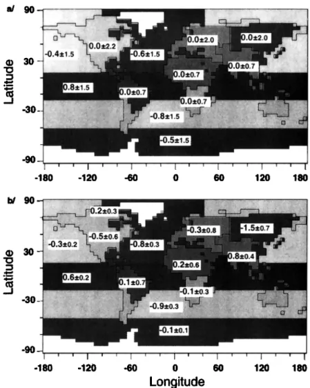
5. Optimized Regional Sources and Sinks

One main advantage of 3-D inversion is that it allows for

estimations of the annual fluxes and errors at continental and

ocean basin scales. However, before presenting regional results, it is important to check the a posteriori spatial correlation between the regions used for inverse calculation.

5.1. A Posteriori Spatial Correlations

The a posteriori coavariance matrix C'm can be converted in spatial correlation between the source regions used for the calculation. A significant a posteriori correlation between two sources means that atmospheric measurements cannot separate the two fluxes. In other words, two regions presenting a significative correlation have to be summed in the results because we only infer information about the sum of their fluxes. The sign of the correlation, even if not significative also gives important indications. We use 45 unknowns (regional annual fluxes), but 11 are linked, as the sum of GPP and RES is constrained to be zero annualy. Thus the level of meaning for the 45-11-2=32 degrees of freedom of our problem is 0.45 (P=0.01). A posteriori correlation between regions are presented in Table 5.

The only sgnificative correlations occur between DEF and BIO_UPT over tropical Asia (-0.58). This means that we cannot separate these two processes in this region. The sign implies that if DEF flux increases, the BIO UPT flux decreases. For the purpose presentation, we choose to add deforestation source and net land uptake not only in tropical Asia but also in other tropical regions. One can observe some negative insignificant correlations between boreal and temperate regions of the Northern Hemisphere (-0.44 in north Asia). For North America, Europe, and north Asia, results will be presented as the sum of boreal and temperate fluxes.

One can also notice the anticorrelation between seasonal cycle and net uptake over Europe and North America (B6/U6 and B2/U2), which means that somehow a large seasonal cycle induces a large uptake over these two regions. For ocean regions we choose to keep three regions in the Southern Hemisphere and to group the two Pacific regions and the two Atlantic regions together. In conclusion, inferred net fluxes and errors are presented in the following over eight continental and five oceanic regions (Figure 6 and Table 3).

26,170 BOUSQUET ET AL.' METHOD OF INVERSE MODELING OF CO2 ! 0 • • 0 o • i i i • o o i

o