HAL Id: hal-00711212
https://hal-pjse.archives-ouvertes.fr/hal-00711212v2
Preprint submitted on 13 Aug 2012HAL is a multi-disciplinary open access
archive for the deposit and dissemination of sci-entific research documents, whether they are pub-lished or not. The documents may come from teaching and research institutions in France or abroad, or from public or private research centers.
L’archive ouverte pluridisciplinaire HAL, est destinée au dépôt et à la diffusion de documents scientifiques de niveau recherche, publiés ou non, émanant des établissements d’enseignement et de recherche français ou étrangers, des laboratoires publics ou privés.
Economic Comparison and Group Identity: Lessons
from India
Xavier Fontaine, Katsunori Yamada
To cite this version:
Xavier Fontaine, Katsunori Yamada. Economic Comparison and Group Identity: Lessons from India. 2012. �hal-00711212v2�
Economic Comparison and Group Identity: Lessons
from India
∗
Xavier Fontaine
†Katsunori Yamada
‡July 16, 2012
Abstract
The caste issue dominates a large part of India’s social and political life. Caste shapes one’s identity. Furthermore, strong tensions exist between castes. Using subjective well-being data, we assess the role economic comparisons play in this society. We focus on both within and between-castes comparisons. Within-caste comparisons appear to reduce well-being. Comparisons between rival castes are found to decrease well-being three times more. We link these results to two models in which economic comparison triggers the actual caste-based behaviours (castes’ political demands, discrimination).
keywords: Subjective Well-being ; Relative Utility ; Comparison ; Identity ; Caste ; India ; Discrimination ; Panel Data
∗We are grateful to Shinsuke Ikeda, Fumio Ohtake, and Yoshiro Tsutsui for allowing us to use the
“Survey on Preferences toward, and Satisfaction with, Life" of Osaka University. We are also grateful to the CEPREMAP and the India Research Group for providing us the Indian National Sample Survey data. We would like to thank Alpaslan Akay, Andrew Clark, Rakesh Gupta, Clément Imbert, Claudia Senik, Zahra Siddique and Pankaj Verma for their helpful comments. Any remaining error is the sole responsibility of the authors.
†Paris School of Economics. Corresponding author: [email protected] ‡Osaka University, ISER
India is a rare example of a large country endowed with a clear social stratifica-tion. Identity depends deeply on the caste one receives at birth. Caste belonging largely defines one’s position in society and economy.
Strong antagonisms oppose castes. These antagonisms often take the form of discrimination toward low castes, but also translate sometimes into violence. Deprived castes have been claiming, and still claim for quotas in education and in the labour market to compensate for their situation.
The idea one’s utility depends on others’ consumption may explain part of this dynamic. Improvements in the rival castes’ living conditions may decrease one’s utility. Under some conditions, this may lead castes to discriminate against each other. The other way around, some types of relative feelings toward people from the same caste may lead to claims for caste-specific policies (positive discrimination). This paper uses subjective well-being data to quantify the strength of these within and between-castes comparisons. These results are then connected to mod-els explaining caste-based behaviours (political claims, discrimination) on the basis of economic comparison.
We make a joint use of two data sets. The first one is an urban panel survey containing an happiness question. The second one is a large, representative In-dian population survey. This second data set makes it possible to compute the expenditure level in the groups respondents are likely to compare to.
Our main empirical results are threefold. Within-caste comparison appears to affect well-being negatively. Indians also compare to people from the rival castes. Between-castes comparison actually decreases well-being three times more than within-caste comparison. These results are shown to be consistent with the actual based discriminations, and to a weaker extent with the claims for caste-targeting policies.
1
Conceptual Framework
1.1
A Conflictual Caste Society
1Although 3 000 years-old, the caste system continues to play a central role in India. This system divides Indians into four classes (varna) and thousands of small com-munities (jati). This clustering strongly frames social and economic behaviours. Caste, indeed, influences deeply one’s role and position in society (occupation, marriage, to whom one can interact with. . . ).
1
This section substantially draws on Susan Bayly’s 2001 general survey of the recent history of the Indian caste society.
India’s caste structure is actually highly conflictual, and generates massive inequalities. This caste system is indeed not only a clustering: it is a social order-ing. Caste determines the level of pureness of an individual. Impure occupations (cleaning, undertaking . . . ) are reserved to low castes. For an orthodox Hindu from the highest castes, interacting with low-caste members may even soil purity. As a matter of fact, Indians still mostly marry inside their own jati (Munshi and Rosenzweig (2006)).
These social inequalities translates into economic inequalities. The first Indian Constitution (1950) groups the different jati into four broader categories, depend-ing on the level of deprivation and social stigma they face. This typology simplifies the study of caste inequalities, and will be used throughout this paper. First, the Scheduled Castes (“untouchables”, or Dalits) and the Scheduled Tribes (the trib-als), are considered as “impure”. Above them are the Other Backward Castes. Even though the castes composing this latter category are mostly considered as “pure”, they are still below the rest of the population in the caste hierarchy, and suffer from the caste system. Eventually, the rest of the population is categorised as the Other.
In spite of large reservations for the deprived castes in education and adminis-tration since the 50s (Bayly (2001), chapter 7), between-castes economic dispari-ties remain dramatic. In terms of per capita household expenditure, Indians from higher castes consume on average 63 % and 46 % more than, respectively, Sched-uled Tribes and SchedSched-uled Castes 2
, and 27 % more than the Other Backward Castes3
.
This system does not only generate massive inequalities: it is also (and conse-quently) conflictual. A large literature documents the discriminations low-castes’ members suffer from. On the labour market, the persistency of these discrimina-tions has been assessed using both non-experimental (e.g. Banerjee and Knight (1985)) and experimental methods (testing methods: Banerjee et al. (2009), Sid-dique (2011)). Low castes also face discriminations on the housing market4
. The other way around, deprived castes very actively struggle to extend the reservation policies they benefit from, sometimes even asking for quotas in the private sector5
. Symptomatic of these tensions are the violent conflicts – or “caste wars” – arising in rural India on a regular basis 6
. Symptomatic also is the preponderant role of
2
Authors’ computation based on the 2009-10 round of the National Sample Survey, with a sample size of 570 000 individuals.
3
Even in the historically very egalitarian, anti-caste state of Kerala, Deshpande (2000) find caste disparities to drive overall inequalities.
4 Bayly (2001), pp. 359-362 5 Bayly (2001), chapter 7. 6 Bayly (2001), chapter 9, pp. 342-358.
these tensions in India’s political life from Independence onwards7
.
1.2
Theory and Prediction
We consider the following relative utility function:
Ui = βyln(yi) + βcln(ycastei) + βrln(yrivali)
Where yi stands for i’s expenditure ; ycastei represents the i’s caste expenditure
level – typically the average or median. Eventually, yrivali is the expenditure level
in the rival castes. This logarithmic-type of specification is widely used to model relative utility8
.
Between-castes rivalries mostly oppose low castes to higher castes (see section 1.1). Rival castes are thus defined the following way9
:
• (“high”) Other Castes are the rivals of Scheduled Castes, Scheduled Tribes and Other Backward Castes
• Scheduled Castes, Scheduled Tribes and Other Backward Castes are the rivals to the Other Castes
Our first interest lays in the sign of both βcand βr. The sign of βcis hard to predict.
The theories of envy and conspicuous (Veblen (1899), Duesenberry (1949)) posit that an increase in others’ expenditure makes one feel deprived, thus decreasing his well-being. In this case, βc<0 may be negative.
The other way around, well-being may actually increase with caste expendi-ture10
. This may happen when one uses others’ consumption to predict her own future level of expenditure. The higher the level of expenditure in the caste, the higher the expected level of own expenditure. Because her expectations are imr-poving, the individual feels better off (Hirschman and Rothschild (1973) ; see Card et al. (2010) for a formalisation). When this informational effect overwhelms envy, βc >0, but these two effects may also balance each other (βc = 0).
Within-caste insurance mechanisms may also partly compensate the negative feelings triggered by envy ; not forgetting altruism (or fellowship feelings) toward people from the same caste11
.
7
Cf. the rise of the anti-reservation party BJP in the 80s and 90s (Bayly (2001), pp.296-300).
8
See Clark et al. (2008) for a development of the model and a literature review.
9
To some extent, however, some Indians from the Other Backward Castes have considered the Scheduled Tribes as a threat. See Bayly (2001), chapter 9, p.347. Due to the limited size of our sample, this paper sticks to the main picture.
10
We draw here from the rich set of explanations developed in Kingdon and Knight (2007).
11
Envy has often been found to dominate the informational effect in developed countries (Clark et al. (2008) ; Card et al. (2010)). In developing countries, the evidences are mixed (Clark and Senik (2011)).
The impact of rival castes’ expenditure is also hard to predict. The literature often assumes comparison to occur among similar people. In India, however, caste rivalry appears to be important (section 1.1), which suggests that βr <0. Some
signal effect may however also exist. Because occupation is partly determined by caste belonging, castes are complementary rather than substitute, which suggests a positive correlation between rival castes’ expenditure. Improvements in the eco-nomic conditions of one caste may thus act as the a signal for the rival castes as well. In this case, we could also have βr= 0 or βr>0. However, there is obviously
no between-castes informal insurance mechanisms, nor should any “between-rival-castes” fellowship feelings be expected. All in all, we thus consider all the following possibilities:
βc <0 and / or βr <0
βc = 0 and / or βr = 0
βc >0 and / or βr >0
We are also interested in testing the relative magnitudes of the estimated co-efficients. Different relative strengths of βy, βc and βr have different implications
term of behaviour. In annexe 5.1, we develop two simple models. In the first one, each caste struggle to increase the living conditions of its members whenever βy + βc > 0. The intuition is simple: when one’s caste obtains new rights (new
quotas, for instance), it makes him feel envious (when βc<0). At the same time,
this person will also benefit from these new rights. When envy does not overwhelm these personal benefits, this individual has an incentive to fight for his caste. The bigger βy+ βc, the bigger this incentive. We thus test for:
βy+ βc >0 or βy+ βc <0
The difference between the within and between-castes comparison coefficients is also important, as it may explain discrimination (annex 5.1’s second model). When an entrepreneur has to choose between hiring someone from her caste, and hiring someone equally skilled from a rival caste, she will prefer the member from her caste whenever choosing the worker from the rival caste brings less well-being (βr < βc). We thus also test for:
βc > βr or βc < βr
1.3
Previous Findings
A few papers have shown relative concerns to play an important role in India, by studying for instance wedding expenditures (Bloch et al. (2004)) and more widely conspicuous consumption (Khamis et al. (2010)). One paper has specifically assessed the role of caste-based relative concerns in India. Building on hypothetical
choice experiment, Carlsson et al. (2009) bring some insight on this issue. They asked respondents to choose between several hypothetical societies for their children. Each of these societies is characterised by child’s income, grand-child’s caste average income, and society’s average income. From the choices made by the respondents, the authors derive respondents’ preferences.
They find caste’s average income to reduce utility, bringing evidences of nega-tive within-caste comparison. Keeping own and caste’s income constant, society’s average income also affects well-being negatively. The coefficient associated to so-ciety’s income appear to be bigger that the coefficient associated to own caste’s income, making the case that Indians compare even more to the rest of the society (including rival castes) than to people from their own caste.
A few other papers document between-group comparison in other countries. Kingdon and Knight (2007) study income comparison in South Africa, bring-ing evidences of between-races comparison. Jiang et al. (2011) and Akay et al. (2012) focus on the relation between rural-to-urban migrants and urban “natives” in China. All these three papers point out that, whereas within-group comparison affects well-being negatively, between-groups comparison makes people better off. A plausible interpretation for this phenomenon is that the level of income in the other group acts as a strong signal about one’s future income.
2
Empirical Strategy
Estimations are conveyed using two databases jointly. The SPSL is a 3-years micro panel survey incorporating an happiness question, together with socio-demographic and economic information about respondents. In this database, however, we do not have enough data to compute accurate estimates of the median expenditure level in the reference group. These computations are thus achieved using an high-quality, large and representative household survey, the Indian National Sample Survey (NSS).
2.1
Empirical Specification
Our analysis builds on the three following equations:
SWBit = ai+ βXit+ βyln(yit) +βcln(ycasteit) +εit
SWBit = ai+ βXit+ βyln(yit) +βrln(yrivalit) +εit
SWBit = ai+ βXit+ βyln(yit) +βcln(ycasteit) +βrln(yrivalit) +εit
where ln(yit) stands for the natural logarithm of i’s monthly household real
ex-penditure at year t ; Xit stands for a set of socio-demographic characteristics.
The individual-specific intercept ai accounts for the existence of an idiosyncratic
well-being trait.
One could first think about defining ln(ycasteit) (resp. ln(yrivalit)) as the
me-dian 12
household expenditure level in i′s caste (resp. rival castes) at year t.
Remark, however, that the two databases we use distinguish only four castes, leading for instance to only four different values each year for ln(within)it. So scarce variations does not allow to identify any significant effect.
Instead, we focus on the way one compares to people similar to him, both in his caste and in the rival castes. We define “people similar to the respondent” as people sharing her age category, educational level and location, following Ferrer-i-Carbonell’s definition of the reference group (2005).
The variable ln(ycasteit) (resp. ln(yrivalit)) thus is the logarithm of the median
real household expenditure level for those in i’s caste (resp. rival castes) who share i’s level of education, age, and location.
ycasteit = median expenditureit(cityi; educationit; age groupit; own castei)
yrivalit = median expenditureit(cityi; educationit; age groupit; ; rival castesi )
Education is defined along seven categories, from “illiterate” to “graduate and above” (see table 1 for the details). Three age groups are considered, each con-taining 1/3 of the adult population in the cities we study. The happiness survey’s respondents live in six cities: Bangalore, Chennai, Delhi, Hyderabad, Kolkata, Mumbai. In the next subsection, we describe in more detail the data we use for these computations.
2.2
Databases
13We convey our analysis using two databases jointly. The first one is the “Survey on Preferences toward, and Satisfaction with, Life” (hereby SPSL), collected by the Global Center of Excellence program of Osaka University. This survey is a three-years panel collected in six of the ten biggest Indian cities (Delhi, Mumbai, Banga-lore, Chennai, Kolkata, and Hyderabad) in January 2009, 2010 and 2011, covering 1.857, 1.280, and 1.037 respondents respectively. Along with socio-demographic questions, the questionnaire contains the following happiness question:
Overall, how happy would you say you are currently ? Using a scale from 0 -10 where “-10” is “very happy” and “0” is “very unhappy”, how would you rate you current level of happiness ?
12
The use of the median, instead of the average, is motivated by its smaller sensitivity to outliers. See for instance Clark et al. (2009).
13
Given the sample size, computing the median expenditure level in the refer-ence groups requires to use an additional database. We thus make use of the NSSO "Employment and Unemployment survey", a large, representative Indian household survey. The last two waves of this survey have been collected from July 2007 to June 2008, and from July 2009 to June 2010 respectively (with respective sample sizes of about 750.000 and 460.000).
When interviewing an household, the NSS measures the average monthly house-hold expenditure during the previous year. We thus match the January 2008 – June 2008, July 2009 – December 2009, and January 2010 – June 2010 monthly household expenditure information from the NSS with the 2009, 2010, and 2011 waves of the SPSL respectively. In the six cities we study, the sample sizes of these NSS subsets are 9.712, 6.731 and 6.561 respectively. All our computations are conveyed using the weights provided in the NSS. The average number of NSS observations used to compute the median household expenditure level in each reference group for each year can be found under each regression table. When performing the regressions described in the previous sub-section, this number is 31 for the within-caste comparison variable and 25 for the between-castes one.
2.3
Treating the caste variable
The caste variable requires a special attention for two reasons. First, no informa-tion on caste has been collected during the first wave of the SPSL. We thus have to extrapolate this information from the next two waves of data.
Second, a sizeable part of the sample changed their caste between January 2010 and January 2011 (38% of observations actually belong to movers). These changes are surprising, as they do not occur for other variables such as education or gender. We hypothesise these changes to be due to the announcement (May 2010) of the first Caste Census since 1931. Low caste members indeed suffer from a strong stigma. But at the same time, they benefit from caste-targetting policies (mostly quotas in administration and education). For that reason, one may be willing to manipulate her caste identity (from low caste to higher caste or vice-versa), especially when government is known to be collecting this information. Some respondents may have confused the SPSL with this Caste Census, consequently deciding to manipulate their caste identity14
.
For that reason, we define respondents’ castes as they declared it during the wave previous to the announcement of the Caste Census (i.e. the second wave). As a robustness check, we drop all the respondents who changed their caste in the
14
A small literature exists on the manipulation of caste identity to obtain some caste advantages ; see Cassan (2011)
course of the survey (see section 3.3). We obtain the same results as we do with the whole sample, which comforts our strategy.
3
Findings
In a preliminary section (3.1), we discuss the coefficients obtained from a simple happiness regression ; we also study the general impact of comparison when caste is not used to define reference groups. We then study within and between-castes comparison (3.2). Several robustness checks are conveyed to assess the validity of these results (3.3).
3.1
General results
3.1.1 Baseline Regression
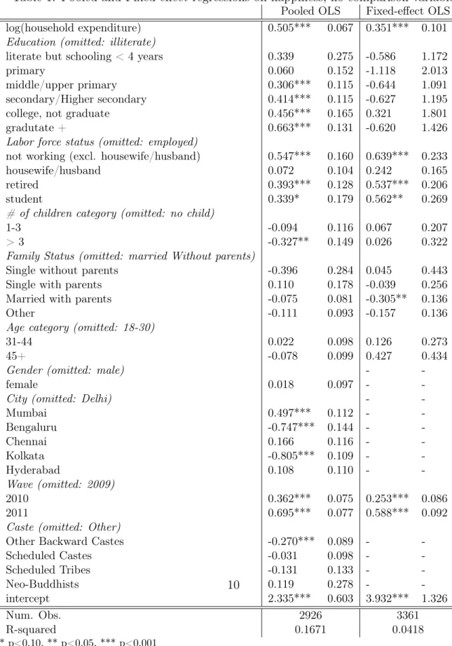
Table 1 displays the results obtained when no comparison variable is included in the regression, both with pooled OLS and fixed-effect OLS. For the sake of conciseness, a general comment on the coefficients is left to the annexe.
The impact of caste deserves some comments. As can be expected, belonging to one of the Other Backward Castes instead of belonging to an higher caste (control group) decreases happiness. However, neither being from a Scheduled Caste, nor being from a Scheduled Tribe has a significant negative impact. This result appears quite puzzling. Interestingly, it is however quite similar to what Linssen et al. (2011) obtain. They find that belonging to a Scheduled Caste/Tribe or to an Other Backward Caste has no significant impact on well-being, as compared to belonging to an higher caste. Still, caste influences expenditure or education which, in turns, affect happiness ; but once we control for those variables affected by caste membership, caste does not appear to affect well-being as much as one could have expected.
3.1.2 General Comparison
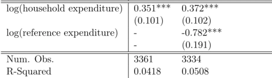
In a first stage, we study the impact of comparison without distinguishing between own and rival castes. The reference group is thus defined accordingly to respon-dents’ age category × education × city. For comparability purpose, we reproduce Table 2’s first column the results obtained when no comparison variable is added to the regression.
The second column displays the impact of own and reference group’s household expenditure. The average number of observations used to calculate reference group expenditures is 65.
Table 1: Pooled and Fixed-effect regressions on happiness, no comparison variable
Pooled OLS Fixed-effect OLS
log(household expenditure) 0.505*** 0.067 0.351*** 0.101
Education (omitted: illiterate)
literate but schooling < 4 years 0.339 0.275 -0.586 1.172
primary 0.060 0.152 -1.118 2.013
middle/upper primary 0.306*** 0.115 -0.644 1.091
secondary/Higher secondary 0.414*** 0.115 -0.627 1.195
college, not graduate 0.456*** 0.165 0.321 1.801
gradutate + 0.663*** 0.131 -0.620 1.426
Labor force status (omitted: employed)
not working (excl. housewife/husband) 0.547*** 0.160 0.639*** 0.233
housewife/husband 0.072 0.104 0.242 0.165
retired 0.393*** 0.128 0.537*** 0.206
student 0.339* 0.179 0.562** 0.269
# of children category (omitted: no child)
1-3 -0.094 0.116 0.067 0.207
> 3 -0.327** 0.149 0.026 0.322
Family Status (omitted: married Without parents)
Single without parents -0.396 0.284 0.045 0.443
Single with parents 0.110 0.178 -0.039 0.256
Married with parents -0.075 0.081 -0.305** 0.136
Other -0.111 0.093 -0.157 0.136
Age category (omitted: 18-30)
31-44 0.022 0.098 0.126 0.273
45+ -0.078 0.099 0.427 0.434
Gender (omitted: male) -
-female 0.018 0.097 -
-City (omitted: Delhi) -
-Mumbai 0.497*** 0.112 - -Bengaluru -0.747*** 0.144 - -Chennai 0.166 0.116 - -Kolkata -0.805*** 0.109 - -Hyderabad 0.108 0.110 - -Wave (omitted: 2009) 2010 0.362*** 0.075 0.253*** 0.086 2011 0.695*** 0.077 0.588*** 0.092
Caste (omitted: Other)
Other Backward Castes -0.270*** 0.089 -
-Scheduled Castes -0.031 0.098 - -Scheduled Tribes -0.131 0.133 - -Neo-Buddhists 0.119 0.278 - -intercept 2.335*** 0.603 3.932*** 1.326 Num. Obs. 2926 3361 R-squared 0.1671 0.0418 * p<0.10, ** p<0.05, *** p<0.001 Standard errors in parenthesis.
Table 2: Fixed-effect OLS regression on happiness, comparison to similar others
Baseline General comparison log(household expenditure) 0.351*** 0.372*** (0.101) (0.102) log(reference expenditure) - -0.782*** - (0.191) Num. Obs. 3361 3334 R-Squared 0.0418 0.0508
* p<0.10, ** p<0.05, *** p<0.001. Standard errors in parenthesis. All controls included. Average number of observations used to compute the reference expenditure level in each cell: 65.
Others’ expenditures appear to reduce happiness sharply, with a significance level of 1%. This result is consistent with what has been found, for instance, in China (Knight and Gunatilaka (2011)), but contrasts with what has been observed in former communists countries during the transition period (Senik 2004, 2008)15
. Remarkably, comparison appears to affect well-being markedly more than house-hold expenditure. Despite the sizeable standard deviation associated to those co-efficients, the difference between their absolute values is almost significant at a 5% level (p-value associated to the two-sided test: .052)16
.
3.2
Within- and Between-Castes Comparisons
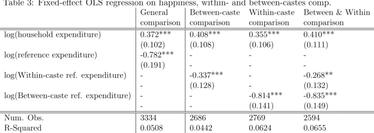
Respondents are likely to compare differently to people from their caste and to people from rival castes. We thus distinguish between within-caste comparisons and between-castes comparisons (see section 2.1). Table 3’s first column replicates the general comparison result we obtained in the previous sub-section. In the second and the third columns, we add the within- and between-castes comparison variables separately. In the fourth column, both of them are included in the same regression.
The fourth column is based on the most complete specification. We thus use it as the baseline for our analysis. The coefficients obtained when putting both the within- and the between-castes variables are however consistent with those obtained in separated regressions (columns 2 & 3).
15
See Clark and Senik (2011) for a general review on the importance of relative deprivation feelings in developing countries.
16
These two coefficients are, in absolute terms, pretty much closer when the regression is performed in pooled OLS (own expenditure: .51 (se: .076), reference expenditure: -.52 (se: .22)). Cf. annexe.
Table 3: Fixed-effect OLS regression on happiness, within- and between-castes comp.
General Between-caste Within-caste Between & Within comparison comparison comparison comparison
log(household expenditure) 0.372*** 0.408*** 0.355*** 0.410***
(0.102) (0.108) (0.106) (0.111)
log(reference expenditure) -0.782*** - -
-(0.191) - -
-log(Within-caste ref. expenditure) - -0.337*** - -0.268**
- (0.128) - (0.132)
log(Between-caste ref. expenditure) - - -0.814*** -0.835***
- - (0.141) (0.149)
Num. Obs. 3334 2686 2769 2594
R-Squared 0.0508 0.0442 0.0624 0.0655
* p<0.10, ** p<0.05, *** p<0.001. Standard errors in parenthesis. Other controls: education, labor force status, number of children, family status, age category, wave. Average number of observations used to compute within and between-castes reference expenditure respectively in each cell for each year: 31 and 25.
Because India is a rapidly changing country, we could expect Indians to use others’ expenditure to predict their own future consumption. The “informational effect”, as describe in section 1.2, could thus be strong enough to compensate for envy. The same way, caste membership defines identity so sharply that we could expect strong caste fellowship feelings, that could overwhelm jealousy. Comparison to similar others within the caste however affects well-being negatively (βc < 0,
5%-level significance). Envy thus appears to be stronger than fellowship feelings and informational effects. This makes the case for marked within-caste relative concerns in India.
In this case where βc < 0, one may not be in favour of policies increasing
consumption in his caste. These policies indeed increase his fellows’ consumption, and consequently his feeling of deprivation. As argued in annex 5.1’s first model, a person will support new policies targeting his caste only if his own benefits exceed the negative impact of envy (βo > βc).In absolute term, within-caste comparisons
have a smaller impact as compared to own expenditure. This result is however only suggestive, as the difference between βo and βc is not significant.
Between-castes comparison appears to have a large, negative, 1%-significant impact on well-being (βr < 0). This result reveals that rival castes’ economic
success enters negatively the well-being function.
Strong between-groups comparisons may have important behavioural implica-tions. This is especially true when between-group comparisons exceed within-caste
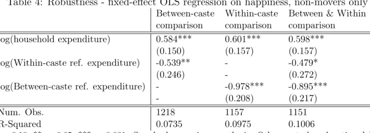
Table 4: Robustness - fixed-effect OLS regression on happiness, non-movers only
Between-caste Within-caste Between & Within comparison comparison comparison
log(household expenditure) 0.584*** 0.601*** 0.598***
(0.150) (0.157) (0.157)
log(Within-caste ref. expenditure) -0.539** - -0.479*
(0.246) - (0.272)
log(Between-caste ref. expenditure) - -0.978*** -0.895***
- (0.208) (0.217)
Num. Obs. 1218 1157 1151
R-Squared 0.0735 0.0975 0.1006
* p<0.10, ** p<0.05, *** p<0.001. Standard errors in parenthesis. Other controls: education, labor force status, number of children, family status, age category, wave. Average number of observations used to compute within and between-castes reference expenditure respectively in each cell: 38 and 14.
comparisons in magnitude (βr> βc). In this latter case, discriminatory behaviours
may appear, since increasing the consumption of someone from a rival caste de-creases well-being, as compared to increasing a fellow’s consumption (see annex 5.1’ second model). More generally, βr > βc would reveal a real between-caste
acrimony.
Between-castes comparisons actually appears to reduce well-being remarkably more than within-caste comparisons (the difference between the two coefficients being significant at a 1% level in a two-sided test). Between-castes comparison even appears to have a stronger absolute impact than own expenditure (5% level)17
.
3.3
Robustness Checks
The validity of the previous results is tested along two lines. Because some respon-dents changed their castes in the course of the survey (cf. section 2.3), we have to check they are not driving the results. In annex, we also made it clear that there is an oversampling of Scheduled Tribes. In a second regression, we run again our analysis without this sub-sample.
We first only keep the respondents we can characterise as non-movers ; that is, those people we observe until the last wave, and who do not change their caste. Table 4 displays the results obtained with this sub-sample. These figures appear to be perfectly similar to what we have previously found.
17
In pooled cross-sections, the between-caste coefficient βr is again much bigger than within-caste
one, βc. Nevertheless, between-caste comparison does not appear to have a larger absolute impact than
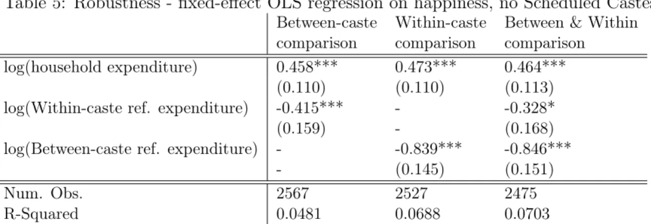
Table 5: Robustness - fixed-effect OLS regression on happiness, no Scheduled Castes
Between-caste Within-caste Between & Within comparison comparison comparison
log(household expenditure) 0.458*** 0.473*** 0.464***
(0.110) (0.110) (0.113)
log(Within-caste ref. expenditure) -0.415*** - -0.328*
(0.159) - (0.168)
log(Between-caste ref. expenditure) - -0.839*** -0.846***
- (0.145) (0.151)
Num. Obs. 2567 2527 2475
R-Squared 0.0481 0.0688 0.0703
* p<0.10, ** p<0.05, *** p<0.001. Standard errors in parenthesis. Other controls: education, labor force status, number of children, family status, age category, wave. Average number of observations used to compute within and between-castes reference expenditure respectively in each cell: 32 and 23.
We then run the analysis again without the Scheduled Tribes. As can be seen in table 5, our results appear to be also robust to their exclusion.
4
Concluding Comments
Relative concerns matter in India. The use of an Indian panel data set reveals that others’ expenditure decreases well-being. This result contrasts with what has been observed in former communists countries during the transition period, but goes in the same direction as those collected in some other developing countries. The pattern we observe is especially consistent with another large, rapidly growing country: China.
Importantly, Indians does not only compare to people from their caste: low castes and high castes appear to compare to each other. Between-castes compar-isons actually appear to decrease well-being about three times more than within-caste comparisons does.
This comparison pattern may have important behavioural implication. A con-tribution of the present paper is to connect these empirical results on group com-parisons with two models of group-based behaviour. We find our results to be consistent with a simple “taste for discrimination” model. The coefficients we ob-tain are also consistent with model explaining groups’ demands for policies, but only to a suggestive extent.
Subjective well-being data appear to be a valuable tool for the study of between-groups relations. Our results suggest for instance that a real acrimony exists
between high and low castes. This type of preferences is hard to capture us-ing the revealed preference approach. The discrimination literature, for instance, has difficulties to distinguish between taste for discrimination and statistical dis-crimination. The subjective well-being approach thus complements the revealed preference approach, by studying more directly the utility function.
Going beyond this “low / high castes” comparison scheme would provide a richer picture of this caste interplay. There could well be some rivalry among low-castes as well, limiting the probability for low castes to act together. Due to the limited size of the happiness sample this paper uses, such a more detailed investigation has to be conveyed in future work.
References
Akay, A., O. Bargain, and K. F. Zimmermann (2012). Relative concerns of rural-to-urban migrants in china. Journal of Economic Behavior & Organization. Banerjee, A., M. Bertrand, S. Datta, and S. Mullainathan (2009, March). Labor
market discrimination in delhi: Evidence from a field experiment. Journal of Comparative Economics 37 (1), 14–27.
Banerjee, B. and J. B. Knight (1985, April). Caste discrimination in the indian urban labour market. Journal of Development Economics 17 (3), 277–307. Bayly, S. (2001). Caste, Society and Politics in India from the Eighteenth Century
to the Modern Age. The New Cambridge History of India. Cambridge University Press.
Bloch, F., V. Rao, and S. Desai (2004). Wedding celebrations as conspicuous consumption: Signaling social status in rural india. Journal of Human Re-sources 39 (3).
Card, D., A. Mas, E. Moretti, and E. Saez (2010, September). Inequality at work: The effect of peer salaries on job satisfaction. NBER Working Papers 16396, National Bureau of Economic Research, Inc.
Carlsson, F., G. Gupta, and O. Johansson-Stenman (2009, January). Keeping up with the vaishyas? caste and relative standing in india. Oxford Economic Papers 61 (1), 52–73.
Cassan, G. (2011). Caste identity manipulation and land ownership in colonial punjab. Working Paper .
Clark, A. E., P. Frijters, and M. A. Shields (2008, March). Relative income, hap-piness, and utility: An explanation for the easterlin paradox and other puzzles. Journal of Economic Literature 46 (1), 95–144.
Clark, A. E., N. Kristensen, and N. Westergård-Nielsen (2009, 04-05). Economic satisfaction and income rank in small neighbourhoods. Journal of the European Economic Association 7 (2-3), 519–527.
Clark, A. E. and C. Senik (2011, February). Will gdp growth increase happiness in developing countries? IZA discussion paper .
Deshpande, A. (2000, May). Does caste still define disparity? a look at inequality in kerala, india. American Economic Review 90 (2), 322–325.
Duesenberry, J. S. (1949). Income, Savings and the Theory of Consumer Behavior. Harvard University Press.
Ferrer-i-Carbonell, A. (2005, June). Income and well-being: an empirical analysis of the comparison income effect. Journal of Public Economics 89 (5-6), 997– 1019.
Hirschman, A. O. and M. Rothschild (1973, November). The changing tolerance for income inequality in the course of economic development; with a mathematical appendix. The Quarterly Journal of Economics 87 (4), 544–66.
Imbert, C. and J. Papp (2011). Government hiring and labor market equilibrium: Evidence from india’s employment guarantee. Working Paper .
Jiang, S., M. Lu, and H. Sato (2011). Identity, inequality, and happiness: Evidence from urban china. World Development.
Khamis, M., N. Prakash, and Z. Siddique (2010, December). Consumption and social identity: Evidence from india. IZA Discussion Papers 5406, Institute for the Study of Labor (IZA).
Kingdon, G. G. and J. Knight (2007, September). Community, comparisons and subjective well-being in a divided society. Journal of Economic Behavior & Organization 64 (1), 69–90.
Knight, J. and R. Gunatilaka (2011). Does economic growth raise happiness in china? Oxford Development Studies 39 (1), 1–24.
Linssen, R., L. van Kempen, and G. Kraaykamp (2011). Subjective well-being in rural india: The curse of conspicuous consumption. Social Indicators Re-search 101, 57–72. 10.1007/s11205-010-9635-2.
Munshi, K. and M. Rosenzweig (2006, September). Traditional institutions meet the modern world: Caste, gender, and schooling choice in a globalizing economy. American Economic Review 96 (4), 1225–1252.
Senik, C. (2004, August). When information dominates comparison: Learning from russian subjective panel data. Journal of Public Economics 88 (9-10), 2099–2123.
Senik, C. (2008, 08). Ambition and jealousy: Income interactions in the ’old’ europe versus the ’new’ europe and the united states. Economica 75 (299), 495– 513.
Siddique, Z. (2011). Evidence on caste-based discrimination. Labour Economics. Veblen, T. (1899). The Theory of the Leisure Class. London: Macmillan, George
Allen and Unwin.
5
Annexes
5.1
Castes’ Political Claims and Discrimination
We provide two models explaining castes’ political claims and discrimination on the basis of relative utility. These models show as simply as possible how much caste-related decisions may depend on the structure of the relative utility function – that is, on the relative magnitudes of the coefficients of βy, βc and βr.
5.1.1 Model 1: Castes’ Political Claims
Demands for positive discrimination constitute a major political fact in India. In a relative utility framework, however, this type of group dynamics does not always emerge. Consider a policy that increases homogeneously consumption in a given caste ; consider a member i of this caste. On the one hand, i benefits from this policy, as it directly increases her consumption. On the other hand, this policy also increases the rest of the castes’ consumption, which will increase i’s feeling of relative deprivation (envy). When this latter phenomenon is too strong, the overall effect of this policy on i’s well-being is negative. A caste will thus demand for a new policy only when this policy’s net impact is positive for a large enough share of its members.
In this model, the members of a given caste vote to decide whether or not they demand for a new policy. The majority rule applies. The policy has a uniform impact on the consumption (it increases consumption by a same amount for all). Utility is:
Ui = βyln(yi) + βcln(ycastei) + βrln(yrivali)
Consistently with the rest of this article, ycastei is the median expenditure level in
i’s caste (or alternatively in the subgroup of the caste i compares to). We denote this median mc.
A policy increasing both this mc and yi by the same amount increases i’s
well-being whenever ∂βyln(yi) ∂yi + ∂βcln(mc) ∂mc >0 ⇔ βyy1 i + βc 1 mc >0
Assume this relation to be true for the median voter (yi = mc). If βy >0 (resp.
βy < 0, resp. βy = 0), then this relation is obviously also true for all those for
whom yi < mc (resp. yi > mc, resp. everyone). That is, if the median voter votes
Thus, the majority votes for this policy whenever βym1c + βcm1c >0
⇔ βy+ βc >0
When βy+ βc >0, demands for caste-based policies may thus appear. The more
positive βy+βcis, the bigger the share of the population in favour of the considered
policy.
5.1.2 Model 2: Taste for Discrimination
Relative utility may also explain discrimination. Discrimination appears whenever someone prefers to hire / buy something to / work with someone from his caste than to do the same with someone from a rival caste, ceteris paribus.
In this model, agent i may choose to interact with someone and get a reward Π, or not to interact at all and get no reward. We write D = 1 if agent i decides to interact, and D = 0 else.
When D = 1, individual i has to choose between two persons. They both have the same characteristics, but one belongs to i’s caste, while the other comes from a rival caste. The person with whom i decides to interact with gets a reward w. Dc = 1 if i choose to interact with the member of his caste, Dc = 0 else. Agent i’s
utility thus is:
Ui= D [Π + Dcβcln(w) + (1 − Dc) βrln(w)]
D = 1 whenever Π + βcln(w) > 0 or Π + βrln(w) > 0. Obviously, i prefers to
interact with the member of his own caste when βcln(w) > βrln(w)
⇔ βc> βr
in which case Dc = 1.
5.2
Data
We provide here a longer description of the two data sets used throughout this article, and compare the basic statistics obtained in the two datasets.
5.2.1 SPSL database
The Global Center of Excellence program of Osaka University has gathered infor-mation on individual’s happiness, monthly expenditure levels, castes, educational attainments, and so forth in its “Survey on Preferences toward, and Satisfaction with, Life." These panel data have been collected via in-person surveys, covering six of the ten biggest Indian cities ; Delhi, Mumbai, Bangalore, Chennai, Kolkata, and Hyderabad. The survey has been conducted in January 2009, 2010 and 2011, covering 1 857, 1 283, and 1 000 respondents respectively. The number of obser-vations usable for regressions will be smaller due to missing information in survey answers, or due to inconsistent answers across the waves.
The data has been collected accordingly to the following design. Each city has been divided into four areas. From each area, we picked up 15 residential sections randomly. Native investigators have been sent to survey five subjects in each residential sections in face-to-face interview. Investigators were free to chose to which door to knock, but they were required to meet two rules: (i) they could not examine a subject living next to the other subjects, (ii) in the collected data set the distributions of gender and age category should be as designed. Regarding the surveys in 2010 and 2011, interviewers went back to the subjects’ places if they had not moved
5.2.2 NSSO Employment and Unemployment survey
The NSSO "Employment and Unemployment survey" is a large, nation-wide and representative survey driven by the NSSO (National Sample Survey Office). This survey is part of a larger survey program, the National Sample Survey, initiated by the Indian government in 1950. This Employment and Unemployment survey takes place roughly every two years.
For the purpose of the present study, we make use of two successive Employment and Unemployment surveys, respectively conducted through the 64th and 66th round of the National Sample Survey. The first took place from July 2007 to June 2008, and the second from July 2009 to June 2010. They collected information on about 570.000 individuals (125.000 households) and 460.000 individuals (100.000) respectively. Even though this is not formally implemented through quarterly stratification, the sampling is designed to be representative at the quarterly level in areas as big as the cities we have at hand (Imbert and Papp (2011)).
Remark that the 64th and 66th rounds of the NSS both contained also a “Con-sumer Expenditure survey”. Both the Employment and Unemployment survey and the Consumer Expenditure survey are representative, but the Consumer Expendi-ture survey also contains detail about each item the household may have consumed. As a counterpart, the size of the sample is considerably smaller (240.000 individuals in 2007-2008 ; 140.000 individuals in 2008-2009) .For that reason, and as detailed data about consumption are not required, we preferred to use the Employment and Unemployment survey.
5.2.3 Comparative statistics – NSS and SPSL
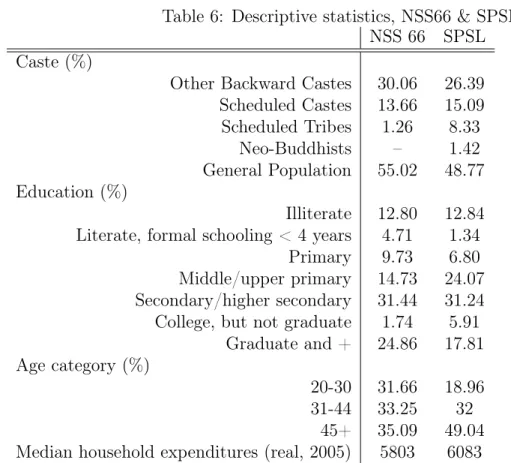
Table 6 compares the ODB and NSS samples with respect to the main population characteristics we are interested in18
.
The median level of household expenditure is quite similar in both samples. The caste distribution in the SPSL appears to be partly imbalanced, with the share of the Scheduled Tribes as a source of concern: they represent 8.33% of the SPSL, and 1.26% of the NSS. The distribution of education is not equal in both samples, but there is no clear shift of general education between them. The sample from the SPSL also appears to be older.
To recover the parameters from the utility function, a perfect representativeness of the sample answering the happiness question is not necessary. The sample used should however resemble the general population reasonably enough to avoid getting a result fallaciously driven by an over-represented sub-population. This is the worry we could have about the Scheduled Tribes, who are clearly over-represented in our sample. For that reason, we test the robustness of our result to the exclusion of these respondents in section 3.3.
18
We restrict the NSS sample to individuals matching the SPSL restrictions: only people older than 20, and living in one of the 6 cities studied in the ODB. For the sake of simplicity, we compare the ODB with the last wave of the NSS.
In the ODB, the sampling procedure is designed to be random at the city level. The number of individuals drawn in each city is however the same by design. To enforce comparability with the NSS, we thus weight each observation accordingly to the share of its city among the 6 cities the respondents live in.
Table 6: Descriptive statistics, NSS66 & SPSL NSS 66 SPSL Caste (%)
Other Backward Castes 30.06 26.39 Scheduled Castes 13.66 15.09 Scheduled Tribes 1.26 8.33 Neo-Buddhists – 1.42 General Population 55.02 48.77 Education (%) Illiterate 12.80 12.84 Literate, formal schooling < 4 years 4.71 1.34
Primary 9.73 6.80 Middle/upper primary 14.73 24.07 Secondary/higher secondary 31.44 31.24 College, but not graduate 1.74 5.91
Graduate and + 24.86 17.81 Age category (%)
20-30 31.66 18.96 31-44 33.25 32
45+ 35.09 49.04 Median household expenditures (real, 2005) 5803 6083
5.3
Commenting the usual set of regressors
This subsection comments at length the coefficients obtained in table 1.We will mostly comment the pooled OLS results here, since socio-demographic character-istics hardly vary during a 3-years time span.
As expected, log real household expenditure has a positive and very significant impact. As compared to being illiterate, education improves monotonically well-being.
The case of the labour force status is of interest. Everything being kept equal (household expenditure included), any situation appears to be better than work-ing, except being “housewife or househusband” (97.6% of people belonging to this category being actually women). The difficult working condition in developing countries certainly drive much of this result. Astonishing however is the impact of “not working”: it appears to be widely preferable not to work (without being housewife/husband) than to be a worker. On this topic, it must however be em-phasised that this status is not equivalent to the fact of being unemployed, that not working but looking for an occupation. In the Hindi version questionnaire, for instance, this answer literally relates to the fact of not working. Since women are over-represented in this category (70%, while they represent only 52% of the sample), we hypothesised that most of these people are women at the head of the household, with another women doing the housekeeping tasks for her (daughter, daughter-in-law, . . . ) ; they thus can declare not to be working, instead of declar-ing they are housewives. When runndeclar-ing this regression separately for men and women, it indeed appears that whereas being "not working" has a significant and positive impact for women, it has a negative insignificant impact for men.
Having between one and three children does not affect happiness, as compared to having no child. Having more than three children, however, significantly de-creases happiness. This pattern is pretty similar to the pattern observed in devel-oped countries. The rest of the family status variables surprisingly does not seem to have any significant impact. Age and gender also appear to have no significant impact. On the contrary, both the living place and the year have strong effects on well-being.
5.4
Replicating the analysis in pooled OLS
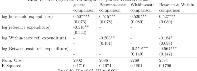
Table 7: OLS regression on happiness, pooled cross-sections
general Between-caste Within-caste Between & Within comparison comparison comparison comparison
log(household expenditure) 0.507*** 0.515*** 0.520*** 0.527***
(0.076) (0.078) (0.080) (0.080)
log(reference expenditure) -0.516** - -
-(0.222) - -
-log(Within-caste ref. expenditure) - -0.203** - -0.184*
- (0.101) - (0.098)
log(Between-caste ref. expenditure) - - -0.559*** -0.564***
- - (0.149) (0.147)
Num. Obs. 2902 2686 2769 2594
R-Squared 0.1710 0.1674 0.1801 0.1796
* p<0.10, ** p<0.05, *** p<0.001
Standard errors in parenthesis. All controls included. OLS standard errors are clustered by (age category × education × city × caste).