HAL Id: hal-01904580
https://hal.archives-ouvertes.fr/hal-01904580
Submitted on 7 Nov 2018
HAL is a multi-disciplinary open access archive for the deposit and dissemination of sci-entific research documents, whether they are pub-lished or not. The documents may come from teaching and research institutions in France or abroad, or from public or private research centers.
L’archive ouverte pluridisciplinaire HAL, est destinée au dépôt et à la diffusion de documents scientifiques de niveau recherche, publiés ou non, émanant des établissements d’enseignement et de recherche français ou étrangers, des laboratoires publics ou privés.
Can SOC modelling be improved by accounting for
pedogenesis?
Peter Finke, Emmanuel Opolot, Jérôme Balesdent, Asmeret Asefaw Berhe,
Pascal Boeckx, Sophie Cornu, Jennifer Harden, Christine Hatté, Elizabeth
Williams, Sebastian Doetterl
To cite this version:
Peter Finke, Emmanuel Opolot, Jérôme Balesdent, Asmeret Asefaw Berhe, Pascal Boeckx, et al.. Can SOC modelling be improved by accounting for pedogenesis?. Geoderma, Elsevier, In press, 338, pp.513-524. �10.1016/j.geoderma.2018.10.018�. �hal-01904580�
1 Title
1
Can SOC modelling be improved by accounting for pedogenesis and weathering in a 2 chronosequence? 3 4 Authors 5
Peter Finke1,*, Emmanuel Opolot1,2, Jerôme Balesdent3, Asmeret Asefaw Berhe4, Pascal Boeckx5,
6
Sophie Cornu3, Jennifer Harden6, Christine Hatté3, Elizabeth Williams4, Sebastian Doettrl7
7 8
Abstract 9
Recent research results suggest that soil organic carbon mineralization and stabilization depend to a 10
substantial degree on the soil geochemistry and the degree of weathering. We hypothesized that 11
this dependence can be translated to decay rate modifiers in a model context, and used data from 12
the Merced chronosequence (CA, U.S.A., 100 yr - 3 Myr), representing a weathering sequence, to 13
test, on a 1000 year time scale, a simple soil organic carbon (SOC) model based on the RothC26.3 14
model concepts. Four information levels were identified: (1) known decay rates per model SOC pool 15
at individual chronosequence locations, obtained by calibrating the model to measured SOC-16
fractions and measured fresh OC-inputs; (2) average decay rates per SOC-pool, corrected per 17
location with rate modifiers based on geochemical proxies; (3) uncorrected average decay rates per 18
SOC-pool; (4) uncorrected average decay rates per SOC-pool and averaged OC-inputs. A lumped root 19
mean square error (RMSE) statistic was calculated per information level. We found that using local 20
measurements of fresh OC-input led to a decrease in RMSE of near 15% relative to information level 21
(4). Applying geochemical rate modifiers led to a further reduction of 20%. Thus, we conclude that 22
1 Department of Soil Management, Ghent University, B-9000 Ghent Belgium; 2 Department of Agricultural
Production, College of Agricultural and Environmental Sciences, Makerere University, Kampala, Uganda; 3
Aix-Marseille Univ, CNRS, INRA, IRD, Coll de France, CEREGE, 13545 Aix-en-Provence, France; 4 University of
California, CA 95343 Merced U.S.A. 5 Department of Applied Analytical and Physical Chemistry, Ghent
University, B-9000 Ghent Belgium; 6 U.S. Geological Survey, CA 94025 Menlo Park U.S.A. 7 Institut für
2
there is a benefit of including geochemical rate modifiers in this SOC-model. We repeated this 23
analysis for a five-pool and a four-pool SOC model that either included or excluded an inert organic 24
matter pool. In terms of the lumped RMSE both models performed similarly, but by comparing 25
measured and simulated percentage Modern Carbon (pMC) for bulk SOC we concluded that 26
measured pMC was best approximated using a four-pool SOC model (without an Inert Organic 27
Matter pool), and that it is likely that a five-pool model including a very slowly decaying pool would 28
further improve model performance. 29
30
Keywords: Soil Organic Carbon; Modelling; Pedogenesis; Weathering; Chronosequence 31
32
1. INTRODUCTION 33
Most earth system models (e.g., Goosse et al., 2010; Kaplan et al., 2011) consider both the input of 34
plant litter in the soil and the decay of Soil Organic Carbon (SOC) as functions of climate, vegetation 35
and land use. It was found (Doetterl et al. 2015; Lawrence et al. 2015; Mathieu et al., 2015) that, 36
under similar vegetation, soil organic carbon mineralization and stabilization is mostly dependent on 37
the soil geochemistry and the degree of weathering (i.e., reactive surface area, texture, Total 38
Reserve of Bases, Si, Fe and Al contents, etc.). However, it is not known how these soil age related 39
attributes quantitatively relate to the age structure (age per type of SOC) of soil organic matter. 40
According to these studies, climate is just one of the drivers. Climate, vegetation as well as 41
geochemical soil composition, resulting from parent material as well as climatic history, may 42
interactively affect the soil microbiological community composition, which are the actual SOC 43
decomposers (e.g. Doetterl et al., 2018). For these experimental findings to be applicable, the effects 44
of mineral weathering and resulting geochemical composition and clay mineralogy on SOC 45
decomposition need to be translated into a model context. This necessarily involves the 46
identification of influential geochemical variables and linking these to model parameters. This study 47
is an attempt to do so in a chronosequence with known gradients in weathering. 48
3
Working hypothesis is that decomposition rates of SOC-pools are different along a chronosequence 49
because of different degrees of weathering of primary minerals and formation of secondary mineral 50
products along this chronosequence, and that these differences can be partly explained by 51
quantitative expressions of weathering and soil geochemistry, and partly by site-specific C-input to 52
the soil. 53
We test this hypothesis on soils from a chronosequence of soils developed on alluvial sediments 54
near Merced, California (Harden 1982, 1987) and use the SoilGen implementation (Finke and 55
Hutson, 2008) of the RothC-concept (Jenkinson and Coleman, 1994; Coleman and Jenkinson, 2005). 56
Essentially, RothC dynamically re-allocates organic matter over different pools having unique 57
decomposition rates (c.f. section 2.2). The implementation in SoilGen follows the RothC-concept, 58
but is discretized over soil depth. RothC was developed to describe SOC-evolution in agricultural 59
field trials covering ca. 150 years and in young parent materials, thus the development domain 60
(time, vegetation and parent materials) is not the same as the application domain in this study. As 61
the temporal range of this chronosequence is far greater than the range for which RothC-pools were 62
defined, the Inert Organic Matter (IOM) pool used in the RothC-model may not be truly “inert”. 63
Radiocarbon studies (Sanderman et al., 2016) have shown that measured ages of soil carbon do not 64
support the presence of truly “inert” organic matter. More generally, the mere existence of Inert 65
Organic Matter has been questioned by the biogeochemistry community (Schmidt et al., 2011). To 66
allow evaluation of the usefulness of IOM as a model pool, we use two versions of this model: with 67
and without IOM. On the Merced chronosequence, SOC-pools have been measured by Doettrl et al. 68
(2018) and mapped onto the pools of C identified in RothC: Resistant Plant Material (RPM), 69
Decomposable Plant Material (DPM), Biomass (BIO), Humus (HUM) and Inert Organic Matter (IOM); 70
described below. 71
The working hypothesis is tested in a four-step approach: 72
1) we apply parameter estimation onto the SOC-model, containing RPM, DPM, BIO, HUM and 73
IOM-pools, at 5 sites of varying age along the chronosequence to obtain site-specific rate 74
4
coefficients. The SOC-model is run for 1000 years on each site to obtain independence of the 75
result on initial pool values; 76
2) we correlate these rates to soil characteristics at these sites to find good candidate 77
(“influencing”) soil properties to be used as rate-modifiers; 78
3) we predict the rate-modifiers with linear regression from the measured soil characteristics 79
at the sites. Linear regression may not capture all possible relationships, but as the data set 80
is small, exploring non-linear methods was not feasible. The predicted rate-modifiers are 81
applied to SoilGen and by comparing simulated to measured pools in extra 1000-year runs, 82
with all other inputs equal to step 1, we evaluate how well the measured DPM, RPM, BIO 83
and HUM pools can be reproduced. This tells us how well rate modifiers perform when local 84
measurements of soil variables are available; 85
4) we evaluate the effect of having site-specific (and likely soil-dependent) organic matter C-86
inputs to simulation quality. 87
As an independent check, we compare measured and calculated radiocarbon (percentage modern 88
carbon) of the calibrated SOC-model for bulk SOC, using the site-specific rate modifiers. This is done 89
for longer time periods (several millenniums) to include the potential effect of old SOC on pMC for 90
those sites in older parts of the chronosequence. 91
92
2. MATERIALS AND METHODS 93
2.1. Merced Chronosequence data summary 94
Soil data were partly collected in 2013, partly taken from previous studies (Harden, 1982, 1987) on a 95
chronosequence of five terrace levels near Merced, California (Table 1) with BSk-climate according 96
to the Köppen-Geiger classification, with average annual temperature of 16.3 °C and 315 mm annual 97
rainfall. The chronosequence spans 0.1 to 3000 ka, where age constraints and associated 98
uncertainties were obtained by stratigraphic correlation, fossils of Hemphillian fauna, 14C, U-series
99
and K-Ar dating and the occurrence of the Gilbert-Gauss magnetic reversal (Marchand and Allwardt, 100
5
1981; Harden, 1987: p. A8). Parent materials are felsic, magmatic and metamorphic alluvial 101
sediments with fine sandy and silty texture, which were field described and analyzed for basic soil 102
properties (texture, color, structure, consistence) allowing calculation of the profile development 103
index (Harden, 1982; Supplementary Information: Table S1). Only the oldest site has substantial 104
amounts of quartz-rich pebbles. Age differences correspond to different weathering intensities, as 105
shown by element ratios, pedogenic iron contents and type of clay minerals (Harden, 1987; Doetterl 106
et al., 2018; Supplementary Information: Table S2). Over the chosen simulation time of 1000 years, 107
we consider the sites to be geomorphologically stable: The sites are on level terrain and surface 108
runoff and water erosion are negligible. Wind erosion is also negligible due to the vegetation cover. 109
Perched water tables of short duration may occur at site PM24II. Over longer time spans this 110
geomorphological stability may not be the case, however. Data used for simulation of soil formation 111
in general and the evolution of soil organic carbon (SOC) are: 112
(i) for model initialization: depth patterns of texture fractions, bulk density, (clay) mineralogy, 113
Cation Exchange Capacity (CEC), root density distribution; 114
(ii) for model calibration and verification: depth patterns of SOC and its fractions (see below) 115
and percentage Modern Carbon (pMC). The pMC is defined as 𝑝𝑀𝐶 = 100 ∗𝐴𝑆𝑁
𝐴𝑂𝑁 , where ASN
116
is the specific activity (decay counts per minute) of the sample normalized to 13C, and A
ON
117
is the specific activity of the oxalic acid standard normalized to 13C;
118
(iii) to satisfy model boundary conditions: evolution of precipitation, potential evaporation, 119
temperature, litter-C input, bioturbation. 120
Data from categories (i) and (ii) are taken from Harden (1987) and Doetterl et al. (2018). In category 121
(iii), weather data were taken from http://www.usclimatedata.com for Merced and the year 2010 122
(precipitation, daily minimum and maximum temperature) and the daily potential evaporation was 123
calculated using the Hargreaves equation (Hargreaves and Samani, 1985). Average rain water 124
composition for 2010 was taken from the National Atmospheric Deposition Program 125
(http://nadp.sws.uiuc.edu/) for Yosemite National Park-Hodgdon Meadow (site CA99). For the 126
6
simulation period (1000 years), we assumed a constant climate, constant vegetation type and 127
constant litter-C input. This model spin-up period and the stable model boundary inputs have the 128
function to obtain independency of the size of the SOC-pools at the end of the simulation from the 129
(unknown) initial situation. 130
To obtain C-input, first the aboveground net primary production (ANPP) was estimated using the 131
Normalized Difference Vegetation Index from 2010-2015 derived from the MOD13Q1 Modis (TERRA) 132
vegetation index from NASA. Carbon biomass was then derived from reference values from 133
literature for grassland in the study region (Berhe, 2012). The ANPP-C was used to estimate the 134
belowground litter production by a standard value for grassland (86% of litter production 135
belowground) as in Kononova (1975). This root litter production was then distributed over the root 136
profile using the root density fractions per depth interval, while the aboveground litter production 137
contributes to the ectorganic layer. 138
Bioturbation, the soil mixing activity by soil meso- and macrofauna or treefalls, is of importance 139
because of the associated vertical transport of soil matter. It was shown to be an important factor in 140
soil horizonation in both field- and simulation studies (e.g. Phillips, 2007; Finke, 2012). Bioturbation 141
also creates macro-pores, which influence CO2-transport (Singer et al., 2001). No bioturbation data is
142
available for the study area. However, Wilkinson et al. (2009) reported values between 10 -50 143
Mg ha-1 y-1 and Gobat (2004) reported values in the range of 13 to 75 Mg ha-1 y-1 for Kansas (Tallgrass
144
Prairie, temperature between 6-19 °C). We decided to take 30 Mg ha-1 y-1 of bioturbation for all
145
chronosequence soils, equally distributed over the root zone compartments and assumed 146
bioturbation independent of soil fertility levels as major bioturbators in the area are mammals 147
(ground squirrels and pocket gophers) that do not consume soil materials. 148
At the sites, from a mass perspective, dust input is minor over the simulation period of 1000 years. 149
There are some indications (Aciego et al., 2017) that Phosphorus (P) inputs by dust may be 150
important. P-input would affect plant biomass production, but as litter production was a simulation 151
input based on measured ANPP, this fertilization effect by P was implicitly taken into account. 152
7 153
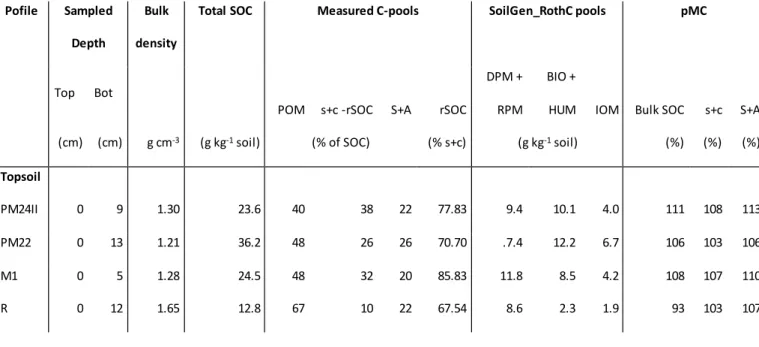
Table 1- General data for Merced chronosequence (Harden, 1982, 1987), WRB2014 classification by the authors. 154 Site name and code WGS84 N / WGS84 W Altitude (m) Sampled depths (cm) topsoil / subsoil Age and uncertainty range (ky) WRB, 2014 USDA, 1975 (great group) Vegetation Post Modesto PM24II 37.62072 / -120.61555 57 0-9 / 19-30 0.1 [0-1] Eutric Gleyic Fluvisols Typic Xerorthents Grassland with scattered oak (Quercus lobata) Post Modesto PM22 37.48854 / -120.52946 56 0-13 / 13-35 3 [1-8.3] Eutric Cambisols Modesto M1 37.52861 / -120.40640 90 0-5 / 22-53 35 [20-70] Haplic Luvisols Typic Haploxeralfs Riverbank R 37.52449 / -120.45434 94 0-12 / 12-39 300 [250-570] Chromic Luvisols China Hat CH 37.46767 / -120.36948 224 2-12 / 12-30 3000 [730-4000] Rhodic Luvisols Typic Palexeralfs 155
SOC fractions were measured in the bulk soil in topsoil and subsoil with the purpose to comply with 156
the four conceptual fractions proposed by Stewart et al. (2008): (i) free particulate organic matter 157
[POM], considered as unprotected; (ii) microaggregate-associated [S+A] SOC, considered as 158
physically protected; (iii) silt- and clay-associated [s+c] SOC, considered as mineral associated, 159
geochemically protected and (iv) nonhydrolyzable [rSOC] SOC equivalent to biochemically protected. 160
The chronosequence soils do not contain carbonates. Physical separation (sieving) techniques 161
(Doetterl et al., 2015) resulted in estimates of particulate organic matter (POM; >250 μm), C 162
associated to stable microaggregates (S+A; 53-250 μm) and C associated to non-aggregated clay and 163
silt (s+c; <53 μm). Additionally, a <63 μm fraction was ultrasonically dispersed (energy level of 22 164
J/mL) from a separate bulk sample and the dispersed solution was then wet sieved over a 63 μm 165
sieve. The suspension < 63 μm was filtered through a 0.45 μm nylon mesh and material >0.45 μm 166
was dried at 40 °C and weighted. This fraction was hydrolyzed with 25mL 6N HCl at room 167
8
temperature for 24 h. The hydrolysis residue after washing was used as estimate of resistant organic 168
carbon (rSOC). The amount of Dissolved Organic Carbon (DOC) was considered negligible under the 169
semi-arid climate at Merced and was not measured. The measured SOC fractions were converted to 170
the C-pools (DPM+RPM), (BIO+HUM) and IOM using the protocol of Zimmermann et al. (2007), c.f. 171
Figure 1. Percentage Modern Carbon (pMC) was measured for topsoil and subsoil in bulk SOC and in 172
the fractions from the physical fractionation. The water used during the fractionation might contain 173
some dissolved organic matter. This would be measured as part of the smallest fraction (s+c; Figure 174
1). DPM/RPM and BIO/HUM ratios for temperate grassland under equilibrium conditions 175
(Zimmerman et al., 2007: table 1: DPM/RPM=0.1271 and BIO/HUM=0.0259) were used to split the 176
pools (DPM+RPM) and (BIO+HUM) obtained from measurements into the RothC-pools. 177
For a more comprehensive description of the collected data we refer to Harden (1987) and Doetterl 178
et al. (2018); for a data summary see Supplementary Information: Table S3. 179
9 181
Figure 1- Analyzed SOC fractions (Stewart et al., 2008; Doetterl et al., 2015) and conversion to four-pool and five-pool 182
RothC-models. indicates distribution over RothC-pools according to Zimmerman et al. (2007) for temperate grassland. 183
RothC-pools are DPM=Decomposable Plant Material; RPM=Resistant Plant Material; BIO=Biomass; HUM=Humus and 184
IOM=Inert Organic Matter. Analytical SOC-fractions are POM=particulate organic Matter; (S+A)= C associated to stable 185
microaggregates (53-250 μm); (s+c)= C associated to non-aggregated clay and silt (<53 μm); and rSOC= resistant organic 186
carbon measured after cold acid hydrolysis (<63 μm). 187
188
2.2. Soil model 189
The effect of mineralogy, climate and vegetation on the depth distribution of SOC over time was 190
simulated with the SoilGen2.15 model (Finke and Hutson, 2008; Opolot and Finke, 2015). 191
SoilGen2.15 simulates flows of water, heat, solutes and CO2 in unconsolidated geomaterials by
192
numerically solving partial differential equations (the Richards equation, heat flow equation, 193
advection-dispersion equation and CO2-diffusion equation respectively), where the column is
194
vertically discretized in equal compartments of five cm thickness in this study. Additionally, transport 195
of solid matter occurs in the form of clay migration (a leaching process) and as a consequence of 196
10
bioturbation (a mixing process). Besides the flow of matter, for each soil compartment various sink 197
and source terms are calculated: (i) Soil texture is modified by physical weathering driven by 198
temperature fluctuations; (ii) soil mineralogical composition is modified by chemical weathering of 199
15 predefined and two user-defined silicate minerals; (iii) equilibriums of calcite and gypsum control 200
the precipitation or dissolution of these salts; (iv) amounts of SOC in the pools RPM, DPM, BIO and 201
HUM are dynamically calculated (see below). These combined processesmimic soil formation (Figure 202
2). The time step for water flow calculations is less than one hour (depending on the rainfall 203
dynamics), for heat flow and physical weathering it is one hour, for solute transport and dissolution 204
chemistry it is less than one day (depending on water flow dynamics) and for the SOC-cycle and 205
chemical weathering it is one day. Bioturbation is calculated for annual time steps. These time steps 206
are matching the dynamics of the individual processes, so that highly dynamic processes (e.g. water 207
flow) as well as relatively slow processes (e.g. weathering of minerals) are simulated efficiently. 208
Several studies confronted outputs of the SoilGen model in multi-millennium simulations to 209
measurements: Finke (2012), Sauer et al. (2012), Yu et al. (2013) Zwertvaegher et al. (2013), Finke et 210
al. (2015) and Keyvanshokouhi et al. (2016) quantified model accuracy at more than 100 locations 211
for SOC, texture, Cation Exchange Capacity, Calcite content, Base Saturation and pH, and concluded 212
fair to good performance. Keyvanshokouhi et al. (2016) concluded that the SoilGen model is suitable 213
for global change effect studies on soils. 214
11 216
Figure 2- Simplified process flowchart of SoilGen model. Copied from Minasny et al. (2015). P=precipitation, 217
PE=evaporation, T=temperature, CDE=convection diffusion equation, CEC=cation exchange capacity , h--K relations 218
describe the relations between soil water pressure head, soil water content and hydraulic conductivity. 219
For the SOC-cycle, the concepts and pools of the RothC26.3 model (Jenkinson and Coleman, 1994; 220
Coleman and Jenkinson, 2005) are implemented for each one of the vertical compartments (in this 221
case, of five cm thickness) and using daily timesteps: 222
Litter arrives at the soil surface as leaf litter or in belowground compartments as root litter. 223
SoilGen uses the simulated root mass density depth pattern (an exponential function declining 224
with depth) to distribute the total root litter over the compartments. The total amount of root 225
and leaf litter is user input per vegetation type. 226
12
All incoming litter is divided by a fixed DPM/RPM ratio (0.67; Jenkinson and Coleman, 1994) into 227
Resistant Plant Material (RPM) and Decomposable Plant Material (DPM) pools. Both these pools 228
decay with rates kRPM and kDPM
229
The resulting decay products from RPM and DPM are split over the Humus (HUM), Biomass (BIO) 230
and mineralized (CO2) pools using the clay content and a fixed BIO/HUM ratio (46/54; Jenkinson
231
and Coleman, 1994). 232
HUM and BIO decay with rates kHUM and kBIO into HUM, BIO and CO2. This cycling of SOC mimics a
233
food web. 234
All rates are modified by factors calculated using temperature and moisture deficit in each soil 235
compartment, as in Jenkinson and Coleman (1994). Both temperature and moisture content are 236
simulated at sub-daily timesteps. The moisture deficit is distributed over the root 237
compartments, using the air-filled porosity per compartment as a proxy for the relative water 238
stress. We assume no other depth dependencies of rates besides those related to differences in 239
temperature and moisture deficit, even though there are indications that these do exist (see 240
Mathieu et al., 2015, but also see Solly et al., 2015 with a contrasting conclusion for Beech forest 241
soils). To mimic effect of the rhizosphere on abundance of micro-organisms, no SOC-decay is 242
assumed to occur below the root zone. SOC-pools may be redistributed over depth as a 243
consequence of bioturbation. 244
The Inert Organic Matter pool (IOM) accounts for stable (non-decaying) organic matter, present 245
at the start of the simulation period and inert during the period covered by the simulation. 246
All SOC-pools in SoilGen contain C, but also the cations and anions taken up by the vegetation via the 247
transpiration stream migrate through the pools, thus finally not only CO2 but also these ions are
248
released (in the soil solution). Parallel to the C-cycle, a 14C cycle is simulated. Litter inputs use the
249
Δ14C of the atmosphere at the year of input t (Hua et al., 2013; Reimer et al., 2013) to construct an
250
extra 14C-related input pool of new litter by LitterC
t * (1+ Δ14Ct/1000), where LitterCt is the litter-C
251
input in year t. The 14C follows the same pathway as C, thus the 14C pools degrade as the SOC-pools,
13
but additionally radioactive decay takes place, which results in dynamic pools representing 253
radiocarbon coined as RPMx, DPMx, BIOx, HUMx and the static pool IOMx. This allows the 254
calculation of Δ14C of total SOC by:
255
∆ 𝐶14 = (RMPx+DPMx+BIOx+HUMx+IOMx
RPM+DPM+BIO+HUM+IOM -1) ∗ 1000 (eq.1)
256
in any subsequent year. For comparison to measurements, pMC is calculated by: 257
𝑝𝑀𝐶 = 100 ∗ ((∆ 𝐶14 /1000) + 1) ∗ 𝑒((𝑦−1950)/(5730/𝐿𝑁(2))) (eq.2), 258
where y is the year of sampling. 259
We apply two variants of this SOC-model (Figure 1): (i) the full five-pool model and (ii) a four-pool 260
model in which IOM is absent and all SOC is subject to decay. The major unknowns that are used in 261
the SOC-module are the decay rates for the four pools. 262
263
2.3. Research Layout and parameter fitting protocol 264
The available data permit calculation of the size of the individual SOC-pools at the five 265
chronosequence sites. The litter-C input and various geochemical properties are also measured at 266
these sites (Doettrl et al., 2018). This data-rich environment permits an analysis of SOC-decay by 267
site-specific model parametrization and calibration, but does not correspond to more common 268
situations where no individual SOC-pools can be obtained from measurements. We therefore 269
consider various information levels, from data-rich to relatively data-poor, to evaluate the quality 270
lost by decreasing data-richness. Figure 3 summarizes the corresponding research layout. 271
At the highest information level (info level 1), a site-specific calibration of the decay rate factors 272
for RPM, DPM, HUM and BIO is performed, using the local profile data to parametrize SoilGen 273
including local estimates of the SOC-input by plant litter. The calibration protocol follows a 274
downstream scheme, which means that the pathway of SOC-decay via RPM and DPM to HUM 275
and BIO determines the calibration order of the decay rate factors. Additionally, rate speeds are 276
considered (slower rates are calibrated first). This results in the calibration sequence 277
kRPM-kDPM-kHUM-kBIO. For each rate, eight equidistant values are taken in a range reported in
14
previous calibration studies (e.g. Yu et al., 2013). The value of the best performing rate factor 279
was obtained by (i) selecting the two consecutive simulated rates with one positive and one 280
negative deviation between measurements and simulations, and (ii) interpolating between these 281
rates to find the rate with an error of near zero. This approach assumes a monotonously 282
decreasing or increasing relation between model error and rate value, which was checked to be 283
true by graphical analysis of the simulations for five sites, eight different values for all four rate 284
coefficients for both the four- and five-pool models, thus for 320 cases. A still better match 285
between simulated and measured pools could have been obtained by an iterative approach to 286
search the optimal parameter value (e.g. by a bisection procedure with a convergence criterion), 287
but this would have added little precision to this study (c.f. Fig. 4) and would have greatly 288
increased computation time. The quality of a calibration run for each pool was expressed via the 289
(absolute) difference between the measured and simulated SOC-pools (Mg ha-1 cm-1 soil) over
290
the same depth intervals combined over topsoil and subsoil. As an example, if measurements 291
apply to 0-9 cm for topsoil and to 19-30 cm for subsoil, values for the same depth intervals were 292
taken from the simulations. SOC is expressed per cm soil to allow comparisons between soils 293
that had unequal sampling layer thickness. 294
The rates obtained by calibration were correlated to geochemical and mineralogical data from 295
the same profiles, to test if these data provide proxies for physico-chemical protection of SOC. 296
We used profile-averages for these proxy-data to avoid weighting for unequal layer thicknesses 297
and because one of the proxies was at the profile-scale. Strong and significant correlations 298
indicate candidate proxies for a next step where rate modifiers are calculated by linear 299
regression. The rate modifiers are applied onto each pool to calculate the loss from that pool by 300
loss=Y*(1-e-x1*x2* k̅̅̅ *tp ) (eq.3),
301
where Y is the size of a pool (RPM, DPM, BIO, HUM) at the start of the (daily) time step for the C-302
cycle sub-model (Mg ha-1 y-1), 𝑘
𝑝
̅̅̅ is the average rate constant (y-1) obtained from the calibrations
303
for pool p; x1 is a (dynamic) rate modifier for the combined effect of moisture, soil cover and 304
15
temperature, fluctuating over time and depth; x2 is an additional rate modifier representing the 305
physico-chemical protection; t is the period of decay (1/365 year). The rate modifier x2 gradually 306
changes over time because of weathering processes affecting geochemical soil properties. The 307
value of x2 is calculated for each site i by: 308
𝑥2𝑖 =𝛽0+ 𝛽1∗𝐺𝑖
𝑘̅ , (eq.4),
309
where βo and β1 are regression coefficients, Gi is the value of the geochemical proxy at i and 𝑘̅ is
310
the average of the calibrated rate constants (y-1) over all locations. In long-term simulations, G
i
311
would be time-dependent to reflect the effect of geochemical weathering processes. In 312
addition, local estimates of the SOC-input by plant litter are input to SoilGen. These simulations 313
applying the rate modifier (one per site) correspond to a second, lower information level (info 314
level 2) where no site-specific rate constants are known but the mineralogy and geochemistry is 315
known and can be used to modify rates. 316
A next lower information level (info level 3) corresponds to the usage of averaged rate constants 317
in combination with local estimates of the SOC-input by plant litter. We distinguished two 318
variants: the literature value for the rate constants (Coleman & Jenkinson, 2005, c.f. Table 2) and 319
the average of the calibrated rate constants. The former is expected to perform worse than the 320
latter as the averages of calibrated constants would give unbiased (average of zero) simulation 321
errors in the study area, but the default rates would likely yield biased (non-zero) simulation 322
errors. 323
The lowest information level (info level 4) corresponds to the usage of average rate constants 324
and of the same SOC-litter inputs at all sites, assuming net primary production does not depend 325
on soil but only on climate. Again, we distinguished two variants: the rates from literature and 326
the averaged rates from calibration. 327
The effects of the information levels on the quality of SOC-simulations over all pools at an individual 328
site is calculated by the site Root Mean Square Error: 329
16 𝑅𝑀𝑆𝐸 = √1 4∑ (𝑆𝑝− 𝑂𝑝) 2 4 𝑝=1 , (eq.5), 330
where Sp and Op are simulated and observed SOC-amounts (Mg ha-1 cm-1 soil) in pool p. We do not
331
consider the difference between measured and simulated IOM because both are either zero (four-332
pool model) or equal (five-pool model) since IOM does not decay (Figure 1). 333
All model simulations covered 1000 years to obtain a stable distribution of SOC over the pools and to 334
avoid an effect of the (unknown) initial SOC-content on final SOC-pools. We compared 100 and 335
1000-year simulations for the young soil PM24II (0.1 ka) and found a minor effect of simulation 336
duration on pool sizes. The SOC-content at the start of the simulations reflected the measured rSOC. 337
In the five-pool model, rSOC was set equal to the IOM-pool, in the four-pool model it was set equal 338
to the initial HUM pool. 339
An over-all index of simulation quality over the five sites is calculated by: 340 𝑅𝑀𝑆𝐸̃ = √1 5∑ (𝑅𝑀𝑆𝐸𝑖) 2 5 𝑖=1 (eq.6) 341
We acknowledge that other accuracy indices could also have been applied, but as we are interested 342
in the decrease of accuracy as a function of information level rather than accuracy itself, we 343
restricted ourselves to RMSE. Adding a penalty for extra parameters needed (at information level 2) 344
could be done by using a statistic such as the Akaike Information Criterion, but this would not inform 345
on the additional cost, which may strongly vary per soil (or weathering) parameter. 346
17 347
Figure 3- Research layout, applied onto both the 4-pool and the 5-pool SOC-model. k* refers to rate constants; RPM, DPM, 348
HUM, BIO and IOM are Soil Organic Carbon (SOC-) pools (described in Fig.1); 𝑅𝑀𝑆𝐸̃ =Root Mean Square Error over 4 pools 349
and 5 sites. Sampling depths for topsoil and subsoil in Table 1. Information levels 1 to 4 are described in section 2.3. 350
351 352
3. RESULTS AND DISCUSSION 353
3.1. Information level 1: Site-specific calibration 354
Primary purpose of the site-specific calibration was to see if rate constant values would differ by 355
location along the chronosequence. This was found to be the case (Table 2). Figure 4 shows that the 356
pool sizes are reproduced accurately. RMSE- and RMSẼ -values in Table 2 indicate that the five-pool 357
model was calibrated slightly more accurately than the four-pool model, but the difference is 358
minimal. In the four-pool model, the kHUM and kBIO indicate slower decay than in the five-pool model,
359
which might be expected because the recalcitrant OC is part of the HUM pool in this model version. 360
kDPM and kRPM did not change because measurements of DPM and RPM are the same for both the
18
four- and five-pool models. At 1000 simulation years, an IOM pool (five-pool model) apparently 362
hardly influences the simulation quality when compared to the four-pool model, even when the IOM 363
equals between 30 and 50% of SOC in the five-pool model simulation results (Figure 4) and the BIO 364
and HUM-pools are consequently smaller in the five-pool model than in the four-pool model. The 365
fastest decomposition rates for fresh organic matter (kRPM and kDPM) are found at the oldest site CH.
366
This can be explained by a relatively high amount of 1:1 (low activity) clay minerals (Supplementary 367
Information: Table S2) that have a weaker capacity to form organo-mineral assemblages and thus 368
result in less protection of relatively fresh (RPM, DPM) SOC than by soils with higher amounts of 2:1 369
minerals (Baldock & Skjemstad, 2000). Slightly faster decay of the HUM and BIO pools is found in the 370
older site R, but only in the site CH with the five-pool model. Finally, it should be noted that 371
differences in total SOC between sites are partly explained by different Litter-C inputs (Table 2; 372
Supplementary Information Table S3; c.f. section 3.3). 373
374
Table 2- Litter-C input, calibrated rate constants (k, expressed in y-1) and RMSE per site for the five-pool and the four-pool
375
model. Italic values in brackets are calibration domain within which the optimal value for k was found. RPM, DPM, HUM, 376
BIO are pools described in Fig.1. C-inputs are based on Doetterl et al., 2018. Default rates RothC-model are taken from 377
Coleman & Jenkinson (2005). 378
Site C-input Mg C ha-1 y-1
5-pool model 4-pool model
kRPM kDPM kHUM kBIO RMSE kRPM kDPM kHUM kBIO RMSE
[0.075; 0.525] [0.100; 1.600] [0.005; 0.035] [0.100; 0.800] [0.075; 0.525] [0.100; 1.600] [0.005; 0.035] [0.100; 0.800] y-1 Mg ha-1 cm-1 y-1 Mg ha-1 cm-1 PM24II 1.3 0.070 0.370 0.008 0.333 0.0246 0.070 0.370 0.005 0.200 0.0090 PM22 1.3 0.059 0.286 0.009 0.370 0.0452 0.059 0.286 0.005 0.217 0.0429 M1 1.0 0.068 0.345 0.009 0.385 0.0093 0.068 0.345 0.010 0.303 0.0260 R 1.2 0.060 0.286 0.023 1.000 0.0265 0.060 0.286 0.012 0.526 0.0283 CH 0.8 0.185 1.000 0.011 0.526 0.0063 0.185 1.000 0.007 0.294 0.0197 RMSẼ RMSẼ
19 Average rate 𝑘̅ 0.089 0.455 0.012 0.526 0.0264 0.089 0.455 0.008 0.303 0.0275 Default k RothC-model 0.30 10.0 0.02 0.66 0.2721 0.30 10.0 0.02 0.66 0.4213 379 380 381
Figure 4- Pool sizes derived from converted measurements (meas; c.f. section 2.1) and from simulations (sim) along the 382
chronosequence for the five-pool model (top) and the four-pool model (bottom) expressed per sampled cm depth. Sampled 383
depth intervals in Table 1. RPM, DPM, HUM, BIO and IOM are pools described in Fig.1. 384
385
3.2. Identification of influencing soil properties 386
Calibrated rate constants were correlated to various measured soil properties to identify candidate 387
properties for rate modifiers (Table 3). Despite the small number of sites, strong and significant 388
correlations were found. Results for the five-pool and four-pool models are similar. It should be 389
noted that the results for the much larger pools RPM and HUM are more relevant than those of the 390
volatile pools of DPM and BIO, which may be more responsive to climate fluctuations. 391
First, important observations are the high and significant correlations between kRPM (and kDPM) and
392
age and the profile development index (PDI, c.f. Supplementary Information; Harden, 1982). The PDI 393
is assessed using basic field soil data, which makes it an easily available rate-modifier in other areas 394
as well. 395
20
Good geochemical candidates for rate modifiers in the five-pool model are 1:1 clay mineral content 396
and 2:1 clay mineral content. The Fe/Si-ratio is a reasonable candidate. These properties are model 397
outputs of SoilGen. Age is of less relevance because it is not a model output, but an input and is not 398
easily estimated for field sites which makes it a less attractive predictor for rate modifiers. 399
The 1:1 clay mineral content correlates positively with all four rates, thus decay of all four pools is 400
faster with higher 1:1 clay mineral content. This is mainly of significance and importance for the 401
large RPM-pool. The positive correlations may be explained by the weak bonding between OM and 402
these low-activity clay minerals and results in less protection of the OM in organo-mineral 403
assemblages. The 2:1 clay mineral content correlates negatively with all four rates, thus decay of all 404
four pools is slower with higher 2:1 clay mineral content. This is explained by the stronger bonding 405
between these high-activity clay minerals and OM, resulting in protection against decomposers, as 406
also stated by others (e.g. Barré et al., 2014; Cuadros, 2017). 407
Fe/Si as well as Al/Si ratios correlate negatively with all four rates, thus soils with higher Fe- or Al-408
content and lower Si-content had slower decay. This holds especially for BIO and to a lesser degree 409
for HUM, and may be explained by OM-stabilization due to organo-mineral interactions at metal 410
surfaces (Kögel-Knabner et al., 2008). Similarly, higher Si contents are positively correlated (though 411
not at high significance) with decay rates, most importantly that of RPM and DPM. 412
In the four-pool model, a significant negative correlation between silt content and kHUM was found.
413
Additionally, BS% correlates negatively (but not at high significance) to kRPM , indicating that soils
414
with a high base saturation have a slower decay of RPM. This might indicate that a higher BS, 415
stimulating biological activity of macrofauna, results in stronger aggregation of the soil and thus 416
better physical protection of RPM from decomposers (Ewing et al., 2006). This effect inverts for kHUM
417
and kBIO (no significant correlations), which may indicate that microfauna can access the HUM and
418
BIO pools. In B-horizons (below the sampled layers in this profile) with stable aggregates, this 419
pattern may inverse to slow decay of SOC, as found by Ewing et al., 2006 for Californian soils. A non-420
significant correlation between KHUM and clay content, additional to the effect already part of the
21
RothC26.3 correction for rates, was found for the four-pool model, which suggests that the 422
RothC26.3 correction for clay content may be improved. 423
424
Table 3- Pearson correlation coefficients between calibrated rate constants (k_RPM, k_DPM, k_HUM and k_BIO, in y-1) and
425
measured soil properties at five sites. Underlined: significant at α=10%; double underlined: significant at 5%; yellow-marked 426
22
field: correlation switched from non-significant to significant or vice versa on change from five-pool to four-pool model. 427
RPM, DPM, HUM, BIO and IOM are defined in Fig.1 and in the introduction. 428
five-pool model four-pool model
Pearson correlations k_RPM k_DPM k_HUM k_BIO IOM k_RPM k_DPM k_HUM k_BIO
kRPM (y -1) 1.00 1.00 kDPM (y -1) 1.00 1.00 1.00 1.00 kHUM (y -1) -0.12 -0.14 1.00 -0.23 -0.25 1.00 kBIO (y -1) -0.05 -0.07 1.00 1.00 -0.09 -0.11 0.88 1.00 IOM (Mg ha-1 cm-1 soil) -0.14 -0.13 -0.67 -0.67 1.00 Age (y) 0.99 0.98 0.02 0.09 -0.21 0.99 0.98 -0.13 0.04
Log Age (y) 0.63 0.61 0.52 0.56 -0.70 0.63 0.61 0.54 0.61
Profile Development Index (-) 0.96 0.95 0.13 0.20 -0.37 0.96 0.95 0.04 0.18
C-input (Mg ha-1 y-1) -0.75 -0.73 -0.56 -0.62 0.63 -0.75 -0.73 -0.38 -0.59
Clay (%) -0.04 -0.06 0.18 0.15 -0.76 -0.04 -0.06 0.76 0.40
Silt (%) 0.63 0.64 -0.55 -0.49 0.66 0.63 0.64 -0.82 -0.64
Sand (%) -0.62 -0.62 0.54 0.50 0.02 -0.62 -0.62 0.16 0.39
Total Reserve of Bases
(cmolc kg-1 cm-1 soil) -0.57 -0.54 -0.40 -0.44 0.55 -0.57 -0.54 -0.47 -0.50
Specific Surface Area treated
(m2 g-1) -0.36 -0.46 -0.41 -0.47 0.02 -0.46 -0.46 0.18 -0.26
Specific Surface Area untreated
(m2 g-1) -0.35 -0.35 -0.29 -0.34 -0.25 -0.35 -0.35 0.38 -0.09 1:1 clay mineral (%) 0.89 0.88 0.32 0.39 -0.43 0.89 0.88 0.14 0.34 2:1 clay mineral (%) -0.92 -0.91 -0.26 -0.33 0.40 -0.92 -0.91 -0.08 -0.29 Si (g/kg) 0.77 0.75 0.45 0.50 -0.51 0.77 0.75 0.32 0.49 Fe/Si -0.47 -0.45 -0.77 -0.81 0.77 -0.47 -0.45 -0.66 -0.82 Al/Si -0.77 -0.74 -0.37 -0.43 0.39 -0.77 -0.74 -0.22 -0.39 P (mg/kg) -0.18 -0.14 -0.65 -0.66 0.67 -0.18 -0.14 -0.74 -0.74 Base Saturation (%) -0.65 -0.68 0.52 0.48 0.06 -0.65 -0.68 0.33 0.43
Cation Exchange Capacity
(cmolc/kg soil) -0.46 -0.45 -0.60 -0.65 0.10 -0.46 -0.45 -0.02 -0.46
23 430
3.3. Simulation quality at different information levels 431
Soil properties with significant correlations to one or more calibrated rate constants (Table 3) were 432
considered suitable candidates to estimate rate modifiers x2 (eq. 3) by linear regression. Thus, using 433
the contents of 1:1 clay minerals and 2:1 clay minerals, the Fe/Si ratio and (for the four-pool model) 434
the silt content, rate modifiers were estimated, the model was run and simulated pools were 435
compared to measured pools (information level 2). Interaction effects of suitable candidate 436
modifiers were also investigated (Fe/Si x 1:1 clay minerals and silt content x 1:1 clay minerals). 437
Results (Figure 5) clearly show that the RMSẼ reduces (and quality increases) with addition of 438
information. The best results were obtained by local calibration (information level 1), and the worst 439
when rates as well as C-inputs were assumed the same at all sites (information level 4). We scaled 440
the RMSẼ at information level 4a (average of measured rates and average of measured C-inputs) to 441
100% in the discussion below. 442
Estimating rate modifiers by geochemical parameters (information level 2) increased RMSẼ by 45-443
50% (compared to information level 1) for the best performing geochemical proxy, the Fe/Si ratio. 444
This ratio is a proxy for bonding in pedogenic hydroxides. Slightly worse results were obtained by 445
using 1:1 or 2:1 clay mineral content to modify rates. Interaction terms of clay mineralogy and Fe/Si 446
ratio did not give better (lower) values of RMSẼ . From the Fe/Si based rate modifiers to the usage 447
of average rates (information level 3a) the RMSẼ increased by about 20%, which illustrates the 448
added value of including geochemical properties in SOC-modelling, and the importance of 449
incorporating the degree of weathering in SOC-modelling. It should be noted that using the default 450
RothC-rates (information levels 4b and 3b) led to a much worse performance in terms of the RMSẼ 451
(30% to 70% higher than at information level 4a), as these default rates added a bias component to 452
the error relative to the usage of locally-averaged rates. Thus, the 20% is a conservative estimate of 453
the gain in quality that can be realized by using rate modifiers, and usage of the default rate 454
constants of RothC introduces large errors in the simulations of the individual pools. Finally, at the 455
24
4th information level (4a) another substantial increase of ca. 15% in the RMSẼ occurred when, in
456
addition to averaged rates, average values for Litter-C inputs are used instead of local values, a 457
situation corresponding to the usage of literature values. Again, the scenario 4b based on default 458
RothC-rates performs much worse than scenario 4a based on the average of the calibrated rates. 459
The decrease in RMSẼ over the information levels from 4 to 1 show that using local estimates of C-460
input contributes positively to simulation quality, though less than when geochemical proxies are 461
used as rate modifiers. C-inputs were found to decrease with greater soil age (Table 2), which is, 462
under the same climate, likely related to less available nutrients with increased degree of 463
weathering. This confirms that the SOC-model should include adequate C-inputs by either 464
accounting for soil fertility in simulating biomass production or by using local measurements. 465
25 466
Figure 5- 𝑅𝑀𝑆𝐸̃ at different information levels: 1=site calibration; 2=site rate modifiers (BS=Base Saturation, c.m.=clay 467
mineral content, interaction a= silt x 1:1 clay mineral content, interaction b= Fe/Si x 1:1 clay mineral content); 3a=average 468
rates; 3b (dotted bars)=default rates RothC26.3; 4a=average rates with average litter-C input; 4b (dotted bars)=default 469
rates RothC26.3 with average C-input. High 𝑅𝑀𝑆𝐸̃ denotes low model performance. Values for 𝑅𝑀𝑆𝐸̃ at information level 470
4a are given at 100% scale. 471
The quality of simulations at all information levels depends on the root depth distribution. Since this 472
is used to distribute belowground litter inputs it will determine the litter input in the sampled soil 473
26
depth compartments. Additionally, the simulation quality depends on the bioturbation. As simulated 474
bioturbation mixes the SOC-pools over the rooted profile, it will decrease the sensitivity of simulated 475
SOC-pools over depth to the root profile. Because the rooting profile and the bioturbation settings 476
were the same for all simulations per site, we assume with confidence that the differences between 477
the information levels are hardly dependent on assumptions on rooting profile and bioturbation. 478
Rate constants (before modification by x1 and x2) in this model study do not vary with depth. Rate 479
modifier x1 depends on temperature and moisture deficit and these do vary with depth. Rate 480
modifier x2 could be estimated per depth compartment using a geochemical proxy, but in this study, 481
we estimated x2 for the whole profile. Since not all geochemical proxies (e.g. newformed clay 482
minerals) can be simulated with SoilGen we used measured values. Although this study shows the 483
value of including geochemical proxies to correct rate constants, the actual gain in quality over long 484
time periods will depend on the accuracy of simulations of these geochemical proxies. For short and 485
recent periods (a few millenniums, c.f. the Fe/Si ratios in Table S2), measured proxy values will 486
suffice. 487
In SoilGen, the uncorrected rate constant is set to zero below the rooting depth, which is below the 488
sampled subsoil layers in this study. Both a constant x2 and no-decay below the rooting zone are
489
over-simplifications and may contribute to the RMSE at all information levels when deeper profiles 490
would be considered. For instance, Mathieu et al. (2015) inventoried turnover rates of deeper 491
carbon (below 20 cm depth) and found different rates for different soil types. Balesdent et al. (2017) 492
measured turnover rates in cultivated soils using 13C labeling techniques, and found turnover rates in
493
subsoils (below 30 cm depth) to be about four times slower than in topsoils. Thus, future models 494
might benefit from exploring the candidate mechanisms that govern dynamic depth adaptation of 495
rate constants. Associations of microbial-mineralogical-root dynamics are likely key to these 496 mechanisms. 497 498 3.4. Radiocarbon 499
27
Values for pMC were measured in topsoil and subsoil bulk samples (Doetterl et al., 2018; 500
Supplementary Information; Table 3) and were also calculated from additional simulations, using the 501
best performing geochemical rate modifiers at information level 2 (i.e. Fe/Si ratio). Simulation 502
periods for these additional simulations were 0.1 ka for site PM24II, 3 ka for PM22 and 10 ka for the 503
other (older) sites. The measured values of pMC (Figure 6) are generally close to or above 100% 504
which indicates that most of the SOC is young. The reason for the exceptional measured value for 505
pMC-bulk soil for the subsoil of site R (300 ka) is that the sample had a large POM content of young 506
age, which was likely due to some root fragments that were, unintendedly, still in the sample in 507
combination with a low total SOC content.
508
Results show that simulations with the four-pool model better match the pMC measurements (RMSE 509
of 10.9%) than those with the five-pool model (RMSE of 30.3%). Topsoil pMC-simulation results are 510
better than those from the subsoil. Assuming an IOM-pool that exists for 10 ka time extent gives a 511
poor estimation of the pMC, which suggests that this SOC cannot be considered inert over several 512
millennia. This was also concluded by Sanderman et al. (2016). Considering IOM to be older than 10 513
ka years leads to worse results. A theoretical limiting case with all IOM as non-radioactive IOM, 514
calculating by setting IOMx in eq.1 equal to zero, is depicted in Figure 6. Thus, it can be concluded 515
that probably the four-pool model is more appropriate for the chronosequence than the five-pool 516
model with inert SOC. However, a modified five-pool model including slow decay of SOC (in a pool 517
replacing IOM) might lead to more accurate results than the results that we obtained. However, the 518
pathways towards such pool then still need to be defined. 519
28 521
Figure 6- Percentage Modern Carbon (pMC) obtained from measurements in bulk soil (solid red) and fractions (solid brown 522
and green) and by simulation with the four-pool model (solid black line, solid rectangles) and five-pool model (dashed black 523
line, open rectangles) for topsoil (left) and subsoil (right). Solid black line with open markers indicate a limiting case without 524
14C in IOM.
525 526
CONCLUSIONS AND OUTLOOK 527
1. Decay rates for the RothC-pools showed significant correlations to both a soil development 528
index (PDI) based on basic field observations as on geochemical weathering metrics. The 529
correlation to PDI would allow rate-modification at large point data sets, as PDI is a function of 530
commonly recorded soil data. This possibility needs to be further explored. 531
2. Over-all, using decay-rate modifiers based on geochemical weathering indices (clay mineralogy 532
and element ratios) significantly improved simulations for SOC storage, but requires measuring 533
and/or modelling these parameters 534
3. Both the five-pool SOC-model, including inert IOM, and the four-pool model without IOM were 535
improved by decay rate modifiers. Comparisons of measured and simulated pMC of bulk SOC 536
samples showed that the inert IOM-pool degrades over periods of time, which provides further 537
evidence that inclusion of an inert pool is not appropriate at millennial timescales. 538
29
4. Local, site specific estimations of C-input generally increased simulation quality, suggesting an 539
impact of the degree of weathering and soil development. Further research should be 540
performed to evaluate this conclusion. 541
5. Major limitation of this study was the small number of sites; thus, results need re-examination at 542
additional sites with varying age and geochemical properties. 543
544
ACKNOWLEDGEMENTS 545
This research was financed in the framework of the BELSPO funded project P7/24 ‘SOGLO’. Special 546
thanks to C. Lawrence (US Geological Survey) for providing a USGS internal review of this 547
manuscript, and to 3 anonymous referees. 548
549
REFERENCES 550
Aciego, S. M., Riebe, C. S., Hart, S. C., Blakowski, M. A., Carey, C. J., Aarons, S. M., Dove, N.C., 551
Botthoff, J.K., Sims, K.W.W., Aronson, E. L. 2017. Dust outpaces bedrock in nutrient supply to 552
montane forest ecosystems. Nature communications, 8, 14800. 553
http://dx.doi.org/10.1038/ncomms14800. 554
Baldock, J.A., Skjemstad, J.O. 2000. Role of the soil matrix and minerals in protecting natural organic 555
materials against biological attack. Organic Geochemistry 31: 697-710. 556
http://dx.doi.org/10.1016/S0146-6380(00)00049-8 557
Balesdent, J., Basile-Doelsch, I., Chadoeuf, J., Cornu, S., Fekiacova, Z., Fontaine, S., Guenet, B., Hatté, 558
C., 2017. Renouvellement de carbone profond des sols cultivés : une estimation par 559
compilation de données isotopiques. Biotechnologie, Agronomie, Société et Environnement 560
21 : 1-9. 561
Barré, P., Fernández-Ugalde, O., Virto, I., Velde, B. and Chenu, C..2014. Impact of phyllosilicate 562
mineralogy on organic carbon stabilization in soils: Incomplete knowledge and exciting 563
prospects. Geoderma 235-236: 382-395. http://dx.doi.org/10.1016/j.geoderma.2014.07.029 564
30
Berhe, A.A. 2012. Decomposition of organic substrates at eroding vs. depositional landform 565
positions. Plant Soil 350: 261-280. http://dx.doi.org/10.1007/s11104-011-0902-z 566
Coleman, K., Jenkinson, D.S., 2005. RothC-26.3: a model for the turnover of carbon in soil. Model 567
Description and Users Guide. November 1999 Issue (Modified April 2005). 568
https://www.rothamsted.ac.uk/sites/default/files/RothC_guide_WIN.pdf (accessed June 569
2017). 570
Cuadros, J., 2017. Clay minerals interaction with microorganisms: a review. Clay Minerals 52: 235– 571
261. http://dx.doi.org/10.1180/claymin.2017.052.2.05 572
Doetterl, Sebastian, Antoine Stevens, Johan Six, Roel Merckx, Kristof Van Oost, Manuel Casanova 573
Pinto, Angélica Casanova-Katny, Cristina Muñoz, Mathieu Boudin, Erick Zagal Venegas, Pascal 574
Boeckx, 2015. Soil carbon storage controlled by interactions between geochemistry and 575
climate. Nature Geoscience 8: 780–783. http://dx.doi.org/10.1038/NGEO2516 576
Doetterl, S., Berhe, A.A., Bodé, S., Fiener, P., Finke, P., Fuchslueger, L., Griepentrog, M., Harden, J., 577
Nadeu, E., Schnecker, J., Six, J., Trumbore, S., Van Oost, K., Vogel, C., Boeckx, P. 2018. Links 578
among warming, carbon and microbial dynamics mediated by soil mineral weathering. 579
Nature Geoscience. http://dx.doi.org/10.1038/s41561-018-0168-7 580
2018Ewing, S.A., Sanderman, J., Baisden, W.T., Wang, Y., Amundson, R. 2006. Role of large-scale soil
581
structure in organic carbon turnover: Evidence from California grassland soils. Journal of 582
Geophysical Research:Biogeosciences 111 issue:G3. 583
http://dx.doi.org/10.1029/2006JG000174 584
Finke, P.A., Hutson, J., 2008. Modelling soil genesis in calcareous löss. Geoderma 145: 462-479. 585
http://dx.doi.org/10.1016/j.geoderma.2008.01.017 586
Finke, P.A, 2012. Modeling the genesis of Luvisols as a function of topographic position in loess 587
parent material. Quaternary International 265: 3-17. 588
http://dx.doi.org/10.1016/j.quaint.2011.10.016 589
31
Finke, P., Samouëlian, A., M. Suarez-Bonnet, B. Laroche and Cornu S. 2015. Assessing the usage 590
potential of SoilGen2 to predict clay translocation under forest and agricultural land uses. 591
European Journal of Soil Science 66(1): 194-205. http://dx.doi.org/10.1111/ejss.12190 592
Gobat, J-M., Aragon, M., Matthey, W., 2004. The Living Soil: Fundamentals of Soil Science and Soil 593
Biology. Science Publishers, Enfield, U.S.A. 602 pp. 594
Goosse, H., Brovkin, V., Fichefet, T., Haarsma, R., Huybrechts, P., Jongma, J., Mouchet, A., Selten, F., 595
Barriat, P.-Y., Campin, J.-M., Deleersnijder, E., Driesschaert, E., Goelzer, H., Janssens, I., 596
Loutre, M.-F., Morales Maqueda, M.A., Opsteegh, T., Mathieu, P.-P., Munhoven, G., 597
Pettersson, E.J., Renssen, H., Roche, D.M., Schaeffer, M., Tartinville, B., Timmermann, A., and 598
Weber, S. L., 2010. Description of the Earth system model of intermediate complexity 599
LOVECLIM version 1.2. Geoscientific Model Development 3: 603-633. 600
https://doi.org/10.5194/gmd-3-603-2010 601
Harden, J.W., 1982. A quantitative Index of Soil Development from Field Descriptions: Examples from 602
a Chronosequence in Central California. Geoderma 28(1): 1-28. 603
https://doi.org/10.1016/0016-7061(82)90037-4 604
Harden, J.W. (editor), 1987. Soils Developed in Granitic Alluvium near Merced, California. U.S. 605
Geological Survey Bulletin 1590A. https://pubs.usgs.gov/bul/1590a/report.pdf 606
Hargreaves, G.H., Samani, Z.A. 1985. Reference crop evapotranspiration from temperature. Appl. 607
Eng. Agric. 1 (2), 96–99. http://dx.doi.org/10.13031/2013.26773 608
Hua, Q., Barbetti, M., Rakowski, A.Z., 2013. Atmospheric radiocarbon for the period 1950–2010. 609
Radiocarbon 55 (4): 2059–2072. http://dx.doi.org/10.2458/azu_js_rc.v55i2.16177 610
Jenkinson, D.S., Coleman, K., 1994. Calculating the annual input of organic matter to soil from 611
measurements of total organic carbon and radiocarbon. European Journal of Soil Science 45, 612
167–174. http://dx.doi.org/10.1111/j.1365-2389.1994.tb00498.x 613
32
Kaplan, J.O., Krumhardt, K.M., Ellis, E.C., Ruddiman, W.F., Lemmen, C., Klein Goldewijk, K., 2011. 614
Holocene carbon emissions as a result of anthropogenic land cover change. The Holocene 21 615
(5): 775–791. http://dx.doi.org/10.1177/0959683610386983 616
Keyvanshokouhi, S., Cornu, S., Samouëlian, A., Finke, P. 2016. Evaluating SoilGen2 as a tool for 617
projecting soil evolution induced by global change. Science of the Total Environment 571: 618
110-123. http://dx.doi.org/10.1016/j.scitotenv.2016.07.119 619
Kögel-Knabner, I., Guggenberger, G., Kleber, M., Kandeler, E., Kalbitz, K., Scheu, S., Eusterhues, K., 620
Leinweber, P. 2008. Organo-mineral associations in temperate soils: Integrating biology, 621
mineralogy, and organic matter chemistry. J. Plant Nutr. Soil Sci. 171: 61–82. 622
http://dx.doi.org/10.1002/jpln.200700048 61 623
Kononova, M.M., 1975. Humus of virgin and cultivated soils. In: Gieseling, J.E. (Ed.), Soil components. 624
I. Organic Components. Springer, Berlin, pp. 475–526. 625
Lawrence, Corey R., Jennifer W. Harden, Xiaomei Xu, Marjorie S. Schulz, Susan E. Trumbore, 2015. 626
Long-term controls on soil organic carbon with depth and time: A case study from the 627
Cowlitz River Chronosequence, WA USA. Geoderma 247–248: 73–87. 628
http://dx.doi.org/10.1016/j.geoderma.2015.02.005 629
Marchand, D.E., and Allwardt, A., 1981, Late Cenozoic stratigraphic units in northeastern San Joaquin 630
Valley, California: U.S. Geological Survey Bulletin 170, 70 p. 631
Mathieu, J., Hatté, C., Parent, E. Balesdent, J., 2015 Deep soil carbon dynamics are driven more by 632
soil type than by climate: a worldwide meta-analysis of radiocarbon profiles. Global Change 633
Biology 21, 4278-4292. http://dx.doi.org/10.1111/gcb.13012 . 634
Minasny, B. Finke, P., Stockmann, U., Vanwalleghem, T. and McBratney, A., 2015. Resolving the 635
integral connection between pedogenesis and landscape evolution. Earth Science Reviews 636
150: 102-120. http://dx.doi.org/10.1016/j.earscirev.2015.07.004 637
33
Opolot, E., Finke, P.A., 2015. Evaluating sensitivity of silicate mineral dissolution rates to physical 638
weathering using a soil evolution model (SoilGen2.25). Biogeosciences 12: 6791-6808. 639
http://dx.doi.org/10.5194/bg-12-6791-2015 640
Phillips, J.D., 2007. Development of texture contrast soils by a combination of bioturbation and 641
translocation. Catena 70 (1), 92-104. http://dx.doi.org/10.1016/j.catena.2006.08.002 642
Reimer, P.J., Bard, E., Bayliss, A., Beck, J.W., Blackwell, P.G., Bronk Ramsey, C., Buck, C.E., Cheng, H., 643
Edwards, R.L., Friedrich, M., Grootes, P.M., Guilderson, T.P., Haflidason, H., Hajdas, I., Hatté, 644
C., Heaton, T.J., Hogg, A.G., Hughen, K.A., Kaiser, K.F., Kromer, B., Manning, S.W., Niu, M., 645
Reimer, R.W., Richards, D.A., Scott, E.M., Southon, J.R., Turney, C.S.M., van der Plicht, J., 646
2013. IntCal13 and MARINE13 radiocarbon age calibration curves 0-50000 years calBP. 647
Radiocarbon 55(4). http://dx.doi.org/10.2458/azu_js_rc.55.16947 648
Sanderman, J., Baisden, W.T., Fallon, S. 2016. Redefining the inert organic carbon pool. Soil Biology 649
and Biochemistry, 92, 149–152. http://dx.doi.org/10.1016/j.soilbio.2015.10.005 650
Sauer, D., Finke, P.A., Schülli-Maurer, I., Sperstad, R., Sørensen, R., Høeg, H.I., Stahr, K. 2012. Testing 651
a soil development model against southern Norway soil chronosequences. Quaternary 652
International 265: 18-31. http://dx.doi.org/10.1016/j.quaint.2011.12.018 653
Schmidt, M.W., M.S. Torn, S. Abiven, T. Dittmar, G. Guggenberger, I.A. Janssens, M. Kleber, I. Kögel-654
Knabner, J. Lehmann, D.A.C. Manning, P. Nannipieri, D.P. Rasse, S. Weiner, S.E.P. Trumbore. 655
2011. Persistence of soil organic matter as an ecosystem property. Nature, 478 (2011), pp. 656
49-56 657
Singer, A.C., Jury, W., Luepranchai, E., Yahng, C.-S., Crowley, D.E., 2001. Contribution of earthworms 658
to PCB bioremediation. Soil Biology & Biochemistry 33, 765–776. 659
http://dx.doi.org/10.1016/S0038-0717(00)00224-8 660
Stewart, C. E., Paustian, K., Plante, A. F., Conant, R. T., Six, J., 2008. Soil carbon saturation: Linking 661
concept and measurable carbon pools. Soil Sci. Soc. Am. J. 72, 379-392 662