The AMBRE Project: [Y/Mg] stellar dating calibration with Gaia

HAL Id: hal-03012071

https://hal.archives-ouvertes.fr/hal-03012071

Submitted on 18 Nov 2020

HAL is a multi-disciplinary open access

archive for the deposit and dissemination of

sci-entific research documents, whether they are

pub-lished or not. The documents may come from

teaching and research institutions in France or

abroad, or from public or private research centers.

L’archive ouverte pluridisciplinaire HAL, est

destinée au dépôt et à la diffusion de documents

scientifiques de niveau recherche, publiés ou non,

émanant des établissements d’enseignement et de

recherche français ou étrangers, des laboratoires

publics ou privés.

The AMBRE Project: [Y/Mg] stellar dating calibration

with Gaia

A. Titarenko, A. Recio-Blanco, P. de Laverny, M. Hayden, G. Guiglion

To cite this version:

A. Titarenko, A. Recio-Blanco, P. de Laverny, M. Hayden, G. Guiglion. The AMBRE Project: [Y/Mg]

stellar dating calibration with Gaia. Astronomy and Astrophysics - A&A, EDP Sciences, 2019, 622,

pp.A59. �10.1051/0004-6361/201833721�. �hal-03012071�

https://doi.org/10.1051/0004-6361/201833721 c ESO 2019

Astronomy

&

Astrophysics

The AMBRE Project: [Y/Mg] stellar dating calibration with Gaia

A. Titarenko

, A. Recio-Blanco

, P. de Laverny

, M. Hayden

, and G. Guiglion

1 _{Laboratoire Lagrange (UMR7293), Université de Nice Sophia Antipolis, CNRS, Observatoire de la Côte d’Azur, BP 4229, 06304}

Nice Cedex 4, France

e-mail: 2chlaidze@gmail.com

2 _{Sydney Institute for Astronomy (SIfA), School of Physics, A28, The University of Sydney, NSW 2006, Australia} 3 _{Center of Excellence for Astrophysics in Three Dimensions (ASTRO-3D), Australia}

4 _{Leibniz-Institut für Astrophysik Potsdam (AIP), 14482 Potsdam, Germany}

Received 26 June 2018/ Accepted 8 November 2018

ABSTRACT

Chemical abundance dating methods open new paths for temporal evolution studies of the Milky Way stellar populations. In this paper, we use a high spectral resolution database of turn-off stars in the solar neighbourhood to study the age dependence of the [Y/Mg] chemical abundance ratio. Our analysis reveals a clear correlation between [Y/Mg] and age for thin disc stars of different metallicities, in synergy with previous studies of solar-type stars. In addition, no metallicity dependence with stellar age is detected, allowing us to use the [Y/Mg] ratio as a reliable age proxy. Finally, the [Y/Mg]–age relation presents a discontinuity between thin and thick disc stars around 9–10 Gyr. For thick disc stars, the correlation has a different zero point and probably a steeper trend with age, reflecting the different chemical evolution histories of the two disc components.

Key words. Galaxy: abundances – Galaxy: disk – Galaxy: stellar content – Galaxy: structure

1. Introduction

Since the advent of stellar astrophysics, the estimation of stellar ages has been a crucial challenge with many fundamental impli-cations. Starting with the historical debate around the age of our Sun, stellar ages have been recognised as clocks of the evolving Universe that we wish to understand. They are the basis of stellar evolution studies, of the stellar properties coded in chemical evo-lution analysis, and more generally a key piece of information of our understanding of any stellar population.

Numerous dating methods have been developed based on dif-ferent physical processes and models. Nuclear cosmochronol-ogy (Hoyle & Fowler 1960;Bland-Hawthorn & Freeman 2014), isochrone fitting (first discovered by Schaltenbrand 1974; Luri et al. 1992; Valls-Gabaud 2014), asteroseismology tech-niques (Pesnell 1987; Guzik et al. 2000), and more indirect chemical proxies of stellar age have been used and applied to very different samples of stars. In particular, for Galactic Archae-ology studies, dating techniques applicable to large numbers of objects are crucial. In this sense, Bayesian isochrone fit-ting methods (Jørgensen & Lindegren 2005), based on the com-parison of the absolute luminosity (or magnitude) of stars and their effective temperatures (or colour) with theoretical models and through Bayesian methods, are among the most commonly used. However, one of the main weaknesses of this approach for Galactic archaeology studies is that it can give reliable results only for stars at the turn-off and the subgiant branch stages, as far as the isochrones are more age sensitive for this type of stars. In addition, precise age estimation from isochrone fitting depends strongly on our knowledge of the stellar distance.

Before the advent of the European Space Agency Gaia mission (Gaia Collaboration 2016b), precise stellar distances were constrained to the solar neighbourhood. The current,

unprecedented precision of the Gaia astrometric measurements allows us to perform the direct distance estimation for about 1.3 billion stars. This opens the way to isochrone fitting age estima-tions for large samples of stars. On the one hand, Gaia ages are already revolutionising our view of the Milky Way stellar popu-lations (Hayden et al. 2018). On the other hand, they will permit the calibration of secondary clocks, like chemical abundance age proxies. These more indirect techniques are important to extend the possibility of stellar dating outside the sphere of the Gaia precise distances and to stars in different stellar evolutionary stages.

This paper focuses on a particular chemical clock: the yttrium to magnesium abundance ratio. Since the studies of da Silva et al. (2012), Nissen (2015), Spina et al. (2016), Tucci Maia et al. (2016), and the recent work of Anders et al. (2018), a correlation of [Y/Mg] with stellar age for solar twins has been noticed. In the work ofFeltzing et al.(2017) a strong correlation is found only for stars with [Fe/H] > −0.5 dex, and Slumstrup et al.(2017) find that this relation also works for solar metallicity stars over the helium-core-burning phase.

Finally, it should be noted that chemical dating can be closely linked to the chemical evolution of a stellar population. In this sense, the comparison of results between thin and thick disc stars can shed a light on the different evolutionary paths of these two disc components. In this paper, a chemical definition of the thin/thick disc populations has been followed. As revealed by several studies inside and outside the solar neighbourhood, thick and thin disc stars seem to separate in two sequences in the [α/Fe] versus metallicity plane (e.g.Adibekyan et al. 2012; Recio-Blanco et al. 2014). Thick disc stars have higher [α/Fe] abundances than thin disc stars of the same metallicity, show-ing also a faster evolution of their [α/Fe] abundance with time (Haywood et al. 2013;Hayden et al. 2018).

Open Access article,published by EDP Sciences, under the terms of the Creative Commons Attribution License (http://creativecommons.org/licenses/by/4.0),

A&A 622, A59 (2019)

The aim of our work is to analyse the age dependence of the [Y/Mg] ratio for turn-off stars in a wide range of metallicities, using a homogeneous and high-resolution spectroscopic sample from the AMBRE project (de Laverny et al. 2012,2013). To this purpose, isochrone fitting ages using astrometric Gaia data from the first data release (Gaia Collaboration 2016a) are used. The high precision of chemical data and of stellar ages, combined with the important number of analysed stars (342 turn-off stars in a wide range of metallicities instead of less than 100, mostly solar twins, for the majority of the previous studies), helps us to further explore the nature and precision of the [Y/Mg] ratio as an age indicator.

In the following section we describe the data set used in this work. Sections 3 and4 present the methodology used for the chemical abundance estimation and the corresponding error analysis. The main results are described in Sects.5and6, while Sect. 7 discusses the differences encountered between the thin and the thick disc populations. The final conclusions are sum-marised in Sect.8.

2. The AMBRE-TGAS data

The Archeologie avec Matisse Basée sur les aRchives de l’ESO (AMBRE) project, established by ESO and l’Observatoire de la Côte d’Azur in 2009 (de Laverny et al. 2013), concerns the parameterisation of the stellar high-resolution spectra of the ESO archives. Stellar spectra collected by three high-resolution spectrographs have already been analysed (FEROS, HARPS, UVES). In this paper, we concentrate on the 4355 parametrised HARPS spectra for which the best stellar Teff, log(g), [Fe/H], and

radial velocity are available (De Pascale et al. 2014). Within the AMBRE database, the HARPS spectra have the highest spectral resolution and contain an important number of stars at the turn-off stage for which isochrone ages can be reliably derived.

The robust identification of the AMBRE/HARPS targets was carefully addressed to overcome the challenges of a cata-logue that is build up from archival data. The 2MASS catacata-logue was chosen as a reference because it offered the advantage of providing photometric information for the targets. The cross-match between the AMBRE/HARPS and 2MASS coordinates was performed using the xcross program (ESO client). In the case of multiple matches within the radius of search (5 arcsec for AMBRE/HARPS), a comparison of the spectroscopic and the photometric effective temperatures was performed. For each match from the 2MASS catalogue, the photometric effective temperature was calculated using the relations of Alonso et al. (1996) and constants from González Hernández & Bonifacio (2009). When there were multiple matches, the objects with the minimal values of |Tphot − TAMBRE| were selected. A total of

2416 different stars along the Hertzprung–Russell diagram were found.

The identified stars were then searched in the Tycho-Gaia Astrometric Solution (TGAS) catalogue. Ages were deter-mined using Bayesian analysis by comparing derived stellar parameters from AMBRE/HARPS data (Teff, [Fe/H], [Mg/Fe],

MK) with theoretical isochrones from the Dartmouth group1

(Dotter et al. 2008), using a method similar to that described byJørgensen & Lindegren(2005). A complete description of the methods employed in this paper to determine ages are provided by the AMBRE-Gaia DR1 catalogue (Hayden et al. 2018). The isochrones are spaced in age from 0 to 15 Gyr, with steps of 100 Myr, in [Fe/H] from −2.0 to +0.6 dex in steps of 0.1 dex,

1 _{http://stellar.dartmouth.edu/models/isolf_new.html}

and from 0.0 to+0.4 dex in [Mg/Fe] in steps of 0.2 dex. The median variance of the age probability distribution function is about 1.2 Gyr for stars younger than 4 Gyr and 1.8 Gyr for stars between 7 and 10 Gyr. After the cross-match with TGAS, a total of 2087 stars remain, from which 502 are turn-off stars.

The absolute magnitude is derived using a Bayesian approach with the parallax information from Gaia DR1 (Perryman et al. 2014), as described in Hayden et al. (2018). The assumptions adopted for the distance determination are a single exponential disc with a scale length of 2.7 kpc and a scale height of 300 pc, and the luminosity function of the solar neighbourhood derived byRobin et al.(2012). To determine the ages, we adopt several simple assumptions. We assume a flat or uniform star formation history, with age spacing provided by the isochrones. The isochrone points are weighted by mass using a Chabrier IMF (Chabrier 2003). We do not assign any assumption based on the metallicity or α-element abundances of the star.

3. Chemical abundance estimation

The abundances of magnesium and yttrium were homoge-neously derived for the complete HARPS-TGAS catalogue. For this purpose, the GAUGUIN method was used (Bijaoui et al. 2012; Guiglion et al. 2016). It is a classical local optimisation method implementing a Gauss–Newton algorithm, based on a local linearisation around a given set of parameters that are asso-ciated with a reference synthetic spectrum (via linear interpola-tion of the derivatives). A few iterainterpola-tions are carried out through linearisation around the new solutions, until the algorithm converges towards the minimum distance between the observed spectrum and the synthetic spectrum library. In practice, we used GAUGUIN together with the stellar parameters independently determined by the algorithm MATISSE (Recio-Blanco et al. 2006; De Pascale et al. 2014) for the AMBRE project. The GAUGUIN code includes a local normalisation step around the selected spectral lines. It is worth noting that GAUGUIN is part of the GSPspec module of the APSIS pipeline (Bailer-Jones et al. 2013) implemented within the GaiaData Processing and Analysis Consortium. In particular, GSPspec is in charge of deriving parameters and abundances from Gaia RVS spectra (Recio-Blanco et al. 2016).

The reference theoretical spectra grid used by GAUGUIN for the magnesium abundance estimation was the GES syn-thetic grid of non-rotating FGKM-type spectra, provided by the GES consortium. It is a high-resolution optical synthetic spectra grid in the 4200–6900 Å wavelength range calculated from the MARCS stellar atmosphere models (Gustafsson et al. 2008) and the GES/Linelist_V5 atomic and molecular line-lists, provided by GES/LineList Group. The microturbulence velocity (ξ) was included in the grid computation by adopting ξ varying as a func-tion of Teff, log(g), and [Fe/H], as adopted in the Gaia-ESO

Sur-vey (Bergemann et al., in prep., based on ξ determinations from literature samples). The [Mg/Fe] variations used for the abun-dance estimation correspond to the [α/Fe] variation of the grid, i.e. ±0.4 dex around the nominal value with a step of 0.2 dex. To be in agreement with the prepared observational HARPS spectra data set, we reduced the resolution of the theoretical spectra to ∼110 000.

Regarding the Y abundance estimations, a specific grid of synthetic spectra has also been computed around the YII lines. We globally followed a procedure similar to the one adopted for the AMBRE grid (de Laverny et al. 2012) except that we also considered an enhancement in yttrium varying over a range

Fig. 1.Example of analysis with the GAUGUIN method. The observed spectrum of HD 9782 is indicated by red circles (Teff= 5980 K,

log(g)= 4.26, [Fe/H] = 0.08, [α/Fe] = −0.01). The solution is shown with blue crosses.

Table 1. Adopted MgI and YII lines, including the ranges used for abun-dance estimation with GAUGUIN.

MgI line (Å) Line range (Å) 5167.3 5166.9 5167.7 5172.6 5172.2 5173.15 5183.6 5183.2 5184.0 5528.4 5528.0 5528.8 5711.0 5710.7 5711.4 YII line (Å) Line range (Å)

4124.19 4124.81 4125.01 4398.01 4397.86 4398.16 4883.68 4883.48 4883.88 4900.12 4899.97 4900.27 4982.13 4981.98 4982.28 5087.42 5087.27 5087.57 5200.41 5200.26 5200.56 5728.89 5728.69 5729.09

of ±1.2 dex around the metallicity with a step of +0.2 dex (leading to 13 different values of [Y/Fe]). We refer to Guiglion et al. (2018) for more details on the computation of this new grid in which we adopted the yttrium line data from Hannaford et al. (1982) and McWilliam et al. (2013; see Table1).

Our selection of Mg spectral lines is based on the work of Mikolaitis et al.(2017). We finally retained the five strong lines presented in Table 1for which the Mg abundance results were less dispersed. In addition, the selection of Y spectral lines was performed to avoid possible blends (Van der Swaelmen, priv. comm.). Table2shows the final line selection, together with the areas for the local spectrum normalization.

The abundances of Y and Mg from each spectrum were calculated as the median value of all available the lines (see Table 1), and the result was flagged with a number of calcu-lated lines. As the first quality cut, we adopted the results for the

Table 2. Detail of the number of analysed stars, the single spectrum cases, and the overlap with reference catalogues for the Y and Mg abundances.

Nstars YII Nstars MgI Description

2050 1795 All calculated abundances

– 1670 In common withMikolaitis et al.(2017) 935 – In common withDelgado Mena et al.(2017)

2416 Stars identified with 2MASS 2087 Subsample containing TGAS stars

502 TO-stars from this TGAS subsample 342 TO-stars with Y and Mg abundances.

spectra with S /N > 30 and standard deviation of median value of the abundance standard deviation smaller than 0.4 dex. The final stellar abundance was then defined as the median abundance value from the multiple spectra of the star. Figure1 illustrates the process of the abundance estimation with GAUGUIN, for a Mg line of the HD 9782 star spectrum (open circles). The cal-culated interpolated synthetic spectra grid for 7 Mg abundance values is colour-coded. The final derived magnesium abundance is shown with X-symbols.

4. Abundance error estimation

We performed the abundance error analysis following three dif-ferent indicators. First, the internal error, given by the line-to-line dispersion per spectra, was considered. The corresponding his-tograms for the Mg and Y abundances are shown in Fig.2. The peak of the distribution is at 0.07 dex for the Mg abundance and 0.12 dex for the Y abundance.

Second, thanks to the significant number of repeats in the catalogue (40% of the stars have one spectrum, and 95% of the stars have been observed less then 30 times; seeDe Pascale et al. 2014), we were able to evaluate the influence of the parame-ter uncertainties in the abundance estimation by looking at the spectrum-to-spectrum dispersion. We recall that the AMBRE project provides atmospheric parameters for each individual spectrum of a particular star. The variations in the atmospheric parameters for the repeated spectra with S/N higher than 30 are lower than 40 K in effective temperature, 0.07 dex in log(g) and 0.03 dex in [Fe/H]. Figure 3 shows the histogram of the Mg and Y abundances dispersion for the repeated spectra. The third quantile of the distribution is at 0.06 dex for Mg and 0.10 dex for Y.

Finally, external errors have been evaluated by comparing our abundance estimations to literature samples having a statis-tically relevant overlap with our data set. Figure4shows the his-togram of the difference between our Mg abundance estimations and theMikolaitis et al.(2014) values. The standard deviation of the difference is 0.08 dex. We note thatMikolaitis et al.(2014) use the same AMBRE parameters as this work, but only the highest S/N spectra per star has been considered, contrary to our approach. In addition, they use a different abundance estimation method, and a different reference spectra grid. Figure5presents the histogram of the differences between our Y abundance esti-mations and theDelgado Mena et al.(2017) values (935 stars in common). In this case, the atmospheric parameters, the abun-dance estimation method and the reference theoretical spectra used by Delgado Mena et al. (2017) differ from those used in this work. The standard deviation of the Y abundance difference is 0.12 dex.

A&A 622, A59 (2019)

Fig. 2.Distribution of standard deviation for the estimation of [Y/H] and [Mg/Fe] from different lines. Top panel: distribution of the standard deviation of [Mg/Fe] for each spectrum, calculated as median value by five spectral lines from Table1. Bottom panel: as above, but for [Y/H] abundances, calculated from eight spectral lines.

Fig. 3.Distribution of standard deviation of [Y/H] and [Mg/Fe]

abun-dances for HARPS stars repeated observations: MgI (red), YII (blue), area in common (grey).

5. Age dependence of the [Y/Mg] abundance

In this section, we analyse the time dependence of the [Y/Mg] abundance as a function of metallicity, age, and disc compo-nent membership (thin or thick disc). The stars have been tagged as belonging to the thin disc, the thick disc, or the high-alpha metal-rich population following the chemical classification of Mikolaitis et al.(2017), which is based on its [Mg/Fe] chemical index.

Fig. 4.Distribution of the difference in [Mg/Fe] abundances between

our AMBRE/HARPS results and those ofMikolaitis et al.(2017).

Fig. 5. Distribution of the difference between [Y/H] abundances

between AMBRE/HARPS and the results from Delgado Mena et al.

(2017).

First, Fig.6presents the abundances of [Fe/H], [Y/H], and [Mg/Fe] as a function of the stellar age for turn-off stars with errors lower than 0.1 dex in abundances. A linear fit for each abundance ratio is presented. Although the [Fe/H] (upper panel) and the [Y/H] abundances (middle panel) present clear negative slopes, both of them present an important dispersion with stellar age (0.23 and 0.21, respectively). The [Mg/Fe] abundance ratio (lower panel) presents a better correlation, with a dispersion of 0.054, that makes the [Mg/Fe] ratio a rather good proxy of the age. However, two different regimes seem to exist: stars younger than and older than ∼10 Gyr (top panel of Fig.6). As shown in previous studies (Haywood et al. 2013,Hayden et al. 2018), the trend of the [Mg/Fe] ratio with stellar age seems to be steeper for thick disc stars (black squares) than for thin disc stars (grey cir-cles). Thus, the [Mg/Fe] abundance cannot be chosen as a robust age indicator for the thin disc population.

Second, Fig.7shows the [Y/Mg] abundance ratio as a func-tion of stellar age for three different subsamples of turn-off stars, progressively increasing the abundance error constraints. The upper panel presents the stars with errors under the level of 0.10 dex for [Mg/Fe] and 0.20 dex for [Y/H] (estimated from the standard deviation of multiple lines). The linear fit corresponds to the thin disc population with ages younger than 10 Gyr. At this step, the 10 Gyr value is only based on the approximative posi-tion separating thin and thick disc stars after the cleaning with the abundance errors. We recall that our thin/thick disc is the one

Fig. 6.Trends of the [Fe/H], [Y/H], and [Mg/Fe] abundances with age

for the complete turn-off sample of AMBRE/HARPS data. Number of stars, coefficients of the fit, and total dispersion of the fit are given in each panel. Thin disc stars are plotted as filled circles, and thick disc stars as filled squares. Opened circles are high-alpha metal-rich objects, following the chemical classification ofMikolaitis et al.(2017).

presented in a trend with age is already clear. With respect to the thin disc population (circles), the thick disc stars (squares) older than 10–11 Gyr seem to be shifted to the thin disc population, although they present an anti-correlation (−0.58 dex) with age. The thin disc versus thick disc differences are studied in greater detail in Sect.7. The middle panel presents a sample with errors lower than 0.05 dex in [Mg/Fe] and 0.10 dex in [Y/H]. The cor-relation increases slightly to −0.62 dex due to smaller dispersion around the thin disc points. It is difficult to disentangle between the spread caused by the abundance and age errors and a possi-ble natural spread due to metallicity because there is a metallicity dependence of the errors. The lower panel of Fig.7, where the error selection is more severe, contains only stars in the metal-licity interval −0.4 dex < [M/H] < 0 dex.

No clear trend with metallicity seems to be present, contrar-ily to the study ofFeltzing et al.(2017). This difference could

Fig. 7.[Y/Mg] vs. stellar age dependence. Top panel: 342 stars with

σYII < 0.2 and σMgI < 0.1 dex; middle panel: 123 turn-off stars with

σYII< 0.1 dex and σMgI < 0.05 dex; bottom panel: 22 turn-off thin disc

stars with σYII < 0.05 dex and σMgI < 0.05 dex. The symbols are as in

Fig.6, and are also colour-coded for the stellar metallicity. The dotted line shows the (Nissen 2015) fit for solar type stars (here c= 0.1 dex); the red solid line (bottom panel) is the fit for the high-precision sample of thin disc stars.

be caused, first, by the spread in the data from Feltzing et al. (2017), which is higher than that used in our selection and can come from the fact that they are using a heterogeneous spec-tra data set (see Table 1 inBensby et al. 2014) and/or the lower spectroscopic resolution of the majority of their data. Second, we have seen that the errors in the abundances are temperature and metallicity dependent, which makes it difficult to compare the two data sets in detail. Also, for metallicities lower than around −0.5 dex, the thin and the thick disc regimes overlap, making the interpretation more complex, especially if the two populations have different slopes of the [Y/Mg] abundance versus age.

Finally, we point out that many of the young and intermedi-ate age thin disc stars are metal-rich objects with very crowded spectra. Therefore, a final selection of a limited sample of stars

A&A 622, A59 (2019)

Fig. 8.Comparison of stellar ages derived from the [Y/Mg] ratio with isochrone fitting ages for a sample of stars not used to infer the [Y/Mg]– age relation. The thick line represents the final correlation; the thin grey line is a diagonal.

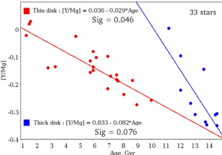
Table 3. Results of the fitting with stellar age for different elements.

fit A B * Age σfit

[Y/Mg]thin 0.036 ± 0.005 −0.029 ± 0.002 0.046

[Y/Mg]thick 0.833 ± 0.006 −0.082 ± 0.002 0.076 Notes. The coefficients for Fe, Y, and Mg abundances are calculated for all turn-off stars with all available ages, the fit of [Y/Mg] is given for the sample of 325 turn-off stars from thin disc (Fig.9).

hotter than 5700 K and having [M/H] less than 0.0 dex was per-formed. This selection avoids problems of blending and contin-uum placement that could be affecting the spectral analysis. In addition, we only kept stars with errors lower than 0.05 dex both in the [Mg/Fe] and in the [Y/H] abundance. This high-precision sample is shown in the lower panel of Fig. 7. Clearly, a clean anti-correlation appears (−0.82) down to 9 Gyr. The final fit of this correlation is

[Y/Mg]_{thin disc}= (0.036 ± 0.005) − (0.029 ± 0.0015) × Age. (1) This fit approaches that ofNissen(2015) andTucci Maia et al. (2016) for solar twins within a slightly lower value of the slope. Reducing the parameter space covered by the data set helps to reduce the internal error spread, including internal biases from one type of star to another.

6. Chemical clock: inverting the [Y/Mg]–age relation.

The clean [Y/Mg]–age relation derived in Sect.5can be used to estimate stellar ages for thin disc stars, replacing isochrone fit-ting outside the ranges of applicability (e.g. main sequence stars outside the turn off). The precision in the derived age can be esti-mated by propagating the errors in Eq. (1). As an example, for a star with [Y/Mg] = (−0.1 ± 0.05) dex the estimation of error in age is around 2 Gyr.

To test this chemical clock we have considered 45 AMBRE/HARPS main sequence and subgiant branch stars slightly outside the conditions of the turn-off definition pro-posed inHayden et al.(2018). We derived isochrone fitting ages for these stars, which were not used in the analysis of Sect. 5,

Fig. 9.[Y/Mg] vs. age fit for thin and thick disc stars.

following the procedure of Hayden et al. (2018). In parallel [Y/Mg]-based ages were derived. Figure8shows the comparison of the two sets of ages. A good correlation appears, with a stan-dard deviation of the difference equal to 2.4 Gyr. The zero point of the difference seems to be within the error for stars younger than 10 Gyr, like those of the thin disc used to derive the rela-tion. In conclusion, the [Y/Mg] abundance ratio can be used as an age proxy for the thin disc stars with reasonable precision, and it can replace more precise age estimations when they are not available.

7. Differences between the thin and the thick disc.

The dependence of [Y/Mg] on stellar age is based on the chem-ical evolution of the analysed population, which means that dif-ferent galactic components could present different trends with age depending, among other things, on their star formation his-tory. In the previous sections, we focus the analysis on thin disc stars, which represent the majority of the AMBRE/HARPS turn-off data.

However, in Sect. 5 we point out the shift that thick disc stars seem to present with respect to the thin disc, causing a dis-continuity in the [Y/Mg] correlation with age. Figure8 shows the high-precision thin disc data set together with the thick disc set, but relaxing the errors to 0.1 dex in [Mg/Fe] and 0.20 dex in [Y/H]. This allows us to include more metal-poor stars in the sample. A similar difference between thick and thin disc appears in the evolution of the [Mg/Fe] ratio with time in the studies ofHaywood et al.(2013) andHayden et al.(2018), highlighting differences in the chemical evolution of these two populations, with the thick disc probably presenting a higher star formation rate. On the other hand, very few literature reports exist regard-ing the [Y/Mg] trend with age,Delgado Mena et al.(2018) find a similar step in the [Y/Mg] for stars with an age older than 10 Gyr. The final derived trends for the thin and thick disc popula-tions are summarised in Table3.

8. Summary and conclusions

The analysis presented in this paper confirms the sensitivity of the [Y/Mg] abundance ratio to stellar age. Thanks to a sam-ple with a high precision of chemical abundances and isochrone ages, the correlation of the [Y/Mg] abundance with age has been evaluated for thin disc and thick disc stars in the solar neighbour-hood.

First, we have shown the importance of reducing the rela-tive errors in the abundances by selecting i) stellar types that are reliable to analyse (e.g. less crowded spectra, easier continuum estimation) and ii) reduced parameter space of the studied sam-ples to minimise internal biases.

Second, a clear correlation between [Y/Mg] and age has been found, with a trend similar to those found in previous studies for solar-type stars (Nissen 2015; Tucci Maia et al. 2016). For the thin disc stars, no particular trend with metallicity seems to exist. We have tested the obtained ratio for stellar age dating through the use of the [Y/Mg] chemical diagnostic, and a precision of around 2 Gyr, in comparison with existing data, was achieved.

Finally, for the first time, we have detected a difference between the thin disc and the thick disc population in the [Y/Mg] dependence with age. As expected from the different chemi-cal evolution history for these two populations, different trends of the [Y/Mg] abundance with age seem to exist. A threshold around 10 Gyr appears in our sample, revealing a chemical dis-continuity between the thick and the thin disc. The population of thick disc stars seems to have a steeper trend with age. To clarify this, more investigations on the thick disc population are needed. We conclude that in the era of large surveys of the Milky Way for which stellar age estimations are a crucial ingredient, chemical diagnostics like the one presented here open new paths for stellar dating.

Acknowledgements. The spectra calculations were performed with the high-performance computing facility MESOCENTRE, hosted by OCA. This work has made use of data from the European Space Agency (ESA) mission Gaia (https://www.cosmos.esa.int/gaia), processed by the Gaia Data Pro-cessing and Analysis Consortium (DPAC;https://www.cosmos.esa.int/ web/gaia/dpac/consortium). We acknowledge financial support form the ANR 14-CE33-014-01. Funding for the DPAC has been provided by national institutions, in particular the institutions participating in the Gaia Multilateral Agreement.

References

Adibekyan, V. Z., Sousa, S. G., Santos, N. C., et al. 2012,A&A, 545, A32 Alonso, A., Arribas, S., & Martinez-Roger, C. 1996,A&A, 313, 873 Anders, F., Chiappini, C., Santiago, B. X., et al. 2018,A&A, 619, A125 Bailer-Jones, C. A. L., Andrae, R., Arcay, B., et al. 2013,A&A, 559, A74 Bensby, T., Feltzing, S., & Oey, M. S. 2014,A&A, 562, A71

Bijaoui, A. 2012, inSeventh Conference on Astronomical Data Analysis, eds. J.-L. Starck, & C. Surace, 2

Bland-Hawthorn, J., & Freeman, K. 2014,The Origin of the Galaxy and Local Group, Saas-Fee Advanced Course (Berlin Heidelberg: Springer-Verlag), 37, 1

Chabrier, G. 2003,PASP, 115, 763

da Silva, R., de Porto Mello, G. F., & Milone, A. C., et al. 2012,A&A, 542, A84 de Laverny, P., Recio-Blanco, A., Worley, C. C., & Plez, B. 2012,A&A, 544,

A126

de Laverny, P., Recio-Blanco, A., Worley, C. C., et al. 2013,The Messenger, 153, 18

Delgado Mena, E., Tsantaki, M., Adibekyan, V. Z., et al. 2017,A&A, 606, A94 Delgado Mena, E., Tsantaki, M., Zh. Adibekyan, V., et al. 2018, inIAU Symp.,

eds. A. Recio-Blanco, P. de Laverny, A. G. A. Brown, et al., 330, 156 De Pascale, M., Worley, C. C., de Laverny, P., et al. 2014,A&A, 570, A68 Dotter, A., Chaboyer, B., Jevremovi´c, D., et al. 2008,ApJS, 178, 89

Feltzing, S., Howes, L. M., McMillan, P. J., & Stonkut˙e, E. 2017,MNRAS, 465, L109

Gaia Collaboration (Brown, A. G. A., et al.) 2016a,A&A, 595, A2 Gaia Collaboration (Prusti, T., et al.) 2016b,A&A, 595, A1 González Hernández, J. I., & Bonifacio, P. 2009,A&A, 497, 497

Guiglion, G., de Laverny, P., Recio-Blanco, A., et al. 2016,A&A, 595, A18 Guiglion, G., de Laverny, P., Recio-Blanco, A., & Prantzos, N. 2018,A&A, 619,

A143

Gustafsson, B., Edvardsson, B., Eriksson, K., et al. 2008,A&A, 486, 951 Guzik, J. A., Kaye, A. B., Bradley, P. A., Cox, A. N., & Neuforge, C. 2000,ApJ,

542, L57

Hannaford, P., Lowe, R. M., Grevesse, N., Biemont, E., & Whaling, W. 1982, ApJ, 261, 736

Hayden, M. R., Recio-Blanco, A., de Laverny, P., et al. 2018,A&A, 609, A79 Haywood, M., Di Matteo, P., Lehnert, M. D., Katz, D., & Gómez, A. 2013,A&A,

560, A109

Hoyle, F., & Fowler, W. A. 1960,ApJ, 132, 565 Jørgensen, B. R., & Lindegren, L. 2005,A&A, 436, 127 Luri, X., Torra, J., & Figueras, F. 1992,A&A, 259, 382

McWilliam, A., Wallerstein, G., & Mottini, M. 2013,ApJ, 778, 149 Mikolaitis, Š., Hill, V., Recio-Blanco, A., et al. 2014,A&A, 572, A33 Mikolaitis, Š., de Laverny, P., Recio-Blanco, A., et al. 2017,A&A, 600, A22 Nissen, P. E. 2015,A&A, 579, A52

Perryman, M., Hartman, J., Bakos, G. Á., & Lindegren, L. 2014,ApJ, 797, 14 Pesnell, W. D. 1987,ApJ, 314, 598

Recio-Blanco, A., Bijaoui, A., & de Laverny, P. 2006,MNRAS, 370, 141 Recio-Blanco, A., de Laverny, P., Kordopatis, G., et al. 2014,A&A, 567, A5 Recio-Blanco, A., de Laverny, P., Allende Prieto, C., et al. 2016,A&A, 585, A93 Robin, A. C., Luri, X., Reylé, C., et al. 2012,A&A, 543, A100

Schaltenbrand, R. A. 1974,A&AS, 18, 27

Slumstrup, D., Grundahl, F., Brogaard, K., et al. 2017,A&A, 604, L8 Spina, L., Meléndez, J., Karakas, A. I., et al. 2016,A&A, 593, A125 Tucci Maia, M., Ramírez, I., Meléndez, J., et al. 2016,A&A, 590, A32 Valls-Gabaud, D. 2014,EAS Pub. Ser., 65, 225