HAL Id: halshs-00272928
https://halshs.archives-ouvertes.fr/halshs-00272928
Submitted on 14 Apr 2008
HAL is a multi-disciplinary open access archive for the deposit and dissemination of sci-entific research documents, whether they are pub-lished or not. The documents may come from teaching and research institutions in France or abroad, or from public or private research centers.
L’archive ouverte pluridisciplinaire HAL, est destinée au dépôt et à la diffusion de documents scientifiques de niveau recherche, publiés ou non, émanant des établissements d’enseignement et de recherche français ou étrangers, des laboratoires publics ou privés.
Monitoring optimistic agents
Nicolas Jacquemet, Jean-Louis Rullière, Isabelle Vialle
To cite this version:
Nicolas Jacquemet, Jean-Louis Rullière, Isabelle Vialle. Monitoring optimistic agents. Journal of Eco-nomic Psychology, Elsevier, 2008, 29 (5), pp.698-714. �10.1016/j.joep.2007.10.002�. �halshs-00272928�
Monitoring optimistic agents
∗Nicolas Jacquemet†, Jean-Louis Rullière‡, Isabelle Vialle
Abstract
Monitoring is typically included in economic models of crime thanks to a probability of detection, constant across individuals. We build on recent results in psychology to argue that comparative optimism deeply affects this standard relation. To this matter, we introduce an experiment involving proper incentives that allow a measurement of optimism bias. Our experiments support the relevance of so-called comparative optimism in decision under risk. In the context of illegal activities, our results provide a guide into costless devices to undermine fraud, through well-designed information campaigns.
JEL classification: C91, C92, D82, H21, H26
Keywords: Optimism, Risk aversion, Monitoring design, Illegal activity, Experimental economics.
1
Introduction
Policymakers often resort to strict monitoring strategies to fight illegal economic activities and to en-courage honesty and law compliance. In this context, decision makers value the potential gains according to both the utility withdrawn from illegality and the probability of being detected (Becker, 1968). If everybody values probabilities without bias the question of the public display of the monitoring policy is irrelevant. This is contradicted, however, by results from psychology, stating that perceptions of this probability can be prone to biases. In particular, experimental evidence shows that people are optimistic about their chances of experiencing favorable future events.
This paper investigates the existence of optimism biases within the context of the monitoring of illegal activities. Our main hypothesis is that people who undertake an illegal activity can be optimistic (pessimistic) about their likelihood to be monitored. Since the detection is a negative event, an optimistic
∗We have greatly benefited from remarks and comments by Nathan Berg, Gerd Gigerenzer, Erik Hoelzl, Philippe Delquié, Claude Montmarquette, Robert Slonim and all participants to the ESA European meeting 2006 in Nottingham, the French Association of Economics (AFSE) annual congress in Paris and the Affect, Motivation and Decision Making International Conference 2006 in Ein Boqeq. We also thank Romain Zeiliger for his help in programming the software used in the experiment. Financial support from the french Agence Centrale des Organismes de Sécurité Sociale (ACOSS), and comments from Alain Gubian, Marianne Pauchet, Nadia Joubert and Bernard Tapie, are gratefully acknowledged.
†Paris School of Economics and University of Paris 1 Panthéon–Sorbonne. ces, 106 Bd. de l’hôpital, 75013 Paris, France.nicolas.jacquemet@univ-paris1.fr
‡Groupe d’Analyse et de Théorie Economique (cnrs, University of Lyon). 93, Chemin des Mouilles, bp167, 69131 Ecully Cedex, France. rulliere@gate.cnrs.fr; vialle@gate.cnrs.fr
(pessimistic) agent thinks she is less (more) likely to be monitored than others are. An optimistic agent hence discerns herself as luckier than others, in the sense of avoiding detection. This could bring those agents to underestimate the probability of detection and thus to undertake more often illegal activities. Inversely, a pessimistic agent is more likely to comply with the legislation due to an overestimation of the risk of detection. According to this hypothesis, observed choices arise from a mix of risk-aversion and optimism. Optimism bias is therefore assessed using a laboratory experiment that allows to disentangle risk aversion and such mis-perceptions.
Our experiment consists in three distinct parts. The first one replicates the protocol originally introduced by Holt and Laury (2002, 2005), which infers the degree of risk aversion from a menu of paired lottery choices. Although the resulting estimates are not noise-free due to order (Harrison et al., 2005) and/or framing effects (Bosch-Domènech and Silvestre, 2006), this standard procedure is only used as a control. Our main focus is rather on identifying optimism (pessimism) bias as regards to a probability of being detected through the two subsequent treatments, called Individual Lottery and Designation. The core decision period remains the same across the two treatments: each subject has to decide on an allocation of a 20 tokens initial endowment between two options. The outcome of the first one is known and certain whereas the second one is random. The wording of the monitoring process however differs between the two treatments. Under Individual Lottery, the probability of detection is announced as such to the subjects, hence underlying the individual nature of monitoring. Under Designation, in contrast, the probability is displayed as the number of participants who will be controlled out of the 20 involved in the session. The parametrization of the options is chosen in such a way that decision periods are two-by-two identical between treatments in terms of the actual risk faced. A fully rational agent should then maintain the same investment decision from one treatment to another. On the opposite, a subject exhibiting comparative optimism (pessimism), should allocate more (less) tokens to the risky option under Designation than under Individual Lottery.
Whatever the treatment, observed investment decisions are in accordance with the expected results. In each treatment, the number of tokens allocated to the risky option decreases in line with the mon-itoring probability, the level of the fine and the degree of risk aversion. Importantly, we also observe significant changes in the investment decisions between the two treatments, hence contradicting the per-fect rationality hypothesis. Subjects change their investment decisions between the two treatments in more than a half of all decision periods. On average, these changes are positive, meaning that subjects are more likely to invest in the illegal (risky) activity under Designation than under Individual Lottery. Econometric analysis confirms that the bias is overall positive and significant. We fail to establish a significant link between attitude toward risk and optimism; those two behavioral motives hence appear essentially orthogonal to one another. Those results extend the empirical evidence from social psychol-ogy to a context involving an explicit link between mis-perception and incentives. As a result, the way the monitoring policy is announced deeply affects the perception of the risk at stake. This advocates a communication policy in which the risk of detection is displayed as an essentially individualized process. The remaining of the paper is organized as follow. An overview of economic and psychology literature devoted to optimism and mis-perception is provided in Section 2. Section 3 describes the experimen-tal design and the procedures used in running the experimenexperimen-tal sessions. Section 4 summarizes our
experimental evidence on comparative optimism bias and the last Section concludes.
2
Related literature
Research in both psychology and economics shows that self-perception is prone to biases: people overestimate the accuracy of both their judgments and their knowledge (miscalibration); they expe-rience systematic biases in the perception of their own characteristics (positive self-image) and they over(under)estimate the likelihood of experiencing (un)favorable events (optimism).
Our paper focuses on the latter, optimism, which refers to an erroneous perception of occurrence probabilities. Two forms of optimism are separately studied in psychology. While Dispositional optimism – traditionally assessed using Scheier et al. (1994)’s Life Orientation Test Revised (LOT-R) – designates the positive perception people exhibit on their own future, comparative optimism characterizes those people that perceive their future more positively than the one of others. Both these biases result in a distortion of the perceived probability as compared to its “objective” value. The first one is however absolute in nature, while the second one is a matter of relative comparisons. In focusing on compara-tive optimism, our paper hence departs from earlier studies on probability distortions (Kahneman and Tversky, 1979; Tversky and Wakker, 1995), devoted to the perception of isolated individuals.
In psychology, comparative optimism is well known as the better-than average effect. Weinstein (1980) relies on a survey asking subjects to rate their likelihood of experiencing some real-life events relative to the average student based on a seven-point scale. People appear to think that (un)pleasant events would happen (less) more often to them than to others. Alicke (1985) applies this same method to positive self-image and obtains that people evaluate themselves (less) more positively than the average student on (un)desirable characteristics.
Such results stemming from research in psychology raise several methodological issues. First, they are based on subjective estimates, rather than on observations of choices among alternatives. The reliability of answers can hence be questioned due to the potential ambiguity of the attribute under evaluation. Furthermore, the results are obtained through verbal statements and without providing subjects with any monetary incentives. Self-evaluations hence come with no guarantee of accuracy.1 These limitations
led economists to develop new experimental tests aimed at improving the reliability of the evidence from psychology. To our knowledge, the new suggested designs focus on positive self-image.
Camerer and Lovallo (1999) is historically the first contribution in this direction. The experiment is based on a market entry game where subjects’ payoffs depend on their rank. Their results show that the participants enter more frequently when the rank is based on the relative performance rather than on a random draw, hence suggesting that participants overestimate their relative performance to the test.
The test performed by Hoelzl and Rustichini (2005) also focuses on self-evaluations of relative perfor-mance. In this case, identification is however derived from a voting procedure on the payment scheme. In the voting step of the experiment, subjects are asked to choose between two rewards: one based on a test appealing to individual skills, the other one based on a random draw. The voting procedure provides evidence for an overestimation of relative performance as soon as more than a half of the sample chooses
1
the relative performance–based reward. Their results show an overestimation of relative performance on easy tests, but an underestimation of relative performance on hard ones.
The main issue with the method introduced by Hoelzl and Rustichini (2005) is the lack of evidence at the individual level. In contrast, Park and Santos-Pinto (2006); Clark and Friesen (2006) suggest a method to elicit individual self-evaluation errors. Beyond some important differences in the design, the two papers share the common feature of eliciting mean beliefs by asking subjects to provide a – rewarded – point forecast about performance. Mitigate evidence arises from those individual assessments. Whereas Park and Santos-Pinto (2006) find clear evidence of a positive self-image, the bias observed by Clark and Friesen (2006) is very thin: overestimation of performance is obtained in only 2 out of the 12 sessions.
Compared to the attention devoted to positive self-image, very few empirical works have been done in economics on optimism biases. The existing studies rely on probability self-evaluations of future outcomes – such as income or longevity. Optimism bias is deduced from comparisons with either current aggregate realizations (Fischhoff et al., 2000) or actual individual realizations (Dominitz and Manski, 1997; Das and van Soest, 1999) when longitudinal data are available. Beyond those field studies, the design of Weinstein (1980) and the LOT-R are up to now the only experimental tools available. Current evidence hence suffers from the limitations mentioned previously. This is a gap this paper aims to fill by introducing an experiment in which comparative optimism is deduced from incentive-based decisions.
3
The experiment
3.1 Experimental designWe explore the optimism bias induced by the monitoring technology through repeated investment deci-sions into a risky activity. The experiment involves three parts. Since we deal with decision making in a risky environment, the first part is aimed at revealing attitudes toward risk. To this matter, we replicate the test originally developed by Holt and Laury (2002, 2005). This consists in a sequence of choices between two lotteries. From one choice to another, the payoffs of the two lotteries are held constant while the probability of an high payoff is progressively increased. The observed switch in the selected lottery hence identifies the risk aversion of the subject.23
The last two parts provide a test of optimism bias based on an investment game, repeated over 22 periods. At the start of each period, each subject is given 20 tokens and decides how many of them to allocate to the risky lottery paying 20 ecu4 per allocated token with probability 1 − p, and 15 − F ecu
with probability p. The remaining tokens give rise to a constant piece-return, set equal to 15 ecu. Those
2
See Appendix A for a summary of the mapping between decisions and risk aversion. 3
It is worth noting that the accuracy of the procedure has received a lot of attention in the last few years. The resulting measure has been shown to be rather noisy – i.e. yielding to a divergence between the answers and the actual preferences towards risk. Such noise essentially comes from order effects (Harrison et al., 2005), since the sequence in which the lotteries are displayed is deterministic, or framing effects (Bosch-Domènech and Silvestre, 2006) induced by the range of lotteries used in the procedure. As explained below, our measure of optimism is however based on comparisons that holds constant the risk faced by the subject. This standard procedure is hence used only to produce an additional covariate; and our main results are unaffected by this noise.
4
two lotteries respectively stand for illegal activity, monitored with probability p and fined by F , and legal activity. In each part, the 22 periods implement all possible combinations between the following parameters: p ∈ {0.05; 0.1; 0.15; 0.2; 0.25; 0.3; 0.35; 0.4; 0.45; 0.5; 0.55} and F ∈ {10; 14}. The occurrence of each combination in a given period is chosen randomly to account for order effects.
Part 2 and 3 only differ according to the way the monitoring is worded. The monitoring associated to the first (risky) lottery is presented as either:
(i) An individual random draw in a ballot box, leading to the low payoff with probability p; or (ii) The (private) designation of n subjects out of the N seated in the room, who will earn the low
payoff.
The two parts are accordingly labeled Individual Lottery – when described as in (i) – and Designation – when described as in (ii). Designation relies on a perfect mapping of the risk faced in the 22 Individual Lottery periods by using all possible combinations between the two levels of the fine, F , and n/N ∈ {0.05; 0.1; 0.15; 0.2; 0.25; 0.3; 0.35; 0.4; 0.45; 0.5; 0.55}. Order effects are accounted for by implementing each treatment as alternatively Part 2 or 3 (see below, Section 3.2 for a precise description of the experimental sessions).
In such a decision-making setting, the information provided to the subjects is of primary importance. First, the subjects are never provided with the full set of parameters. The parameters of the current lottery (i.e. monitoring and fine levels) are rather announced at the beginning of each period. In doing so, we aim at minimizing the effect of subsequent periods on current decision. Second, we get rid of learning effects by providing no feedback on actual monitoring until the end of the session. Last, it is common knowledge that only one period out of the 54 played in the whole experiment will underlie monetary earnings. The paid period is randomly drawn – and privately disclosed to the subjects – at the end of the experiment. This rules out wealth effects, since every decision period has the same ex ante weight in the final wealth of the subjects.
Under those conditions, the 22 periods played under Designation and Individual Lottery treatments are two-by-two identical in terms of decision theory. The risk faced by the subjects, in particular, is held constant through the parametrization p = n/N . Rational behavior would therefore lead to no variation in investment decisions. Of course, treatments are indeed different as regards to perception motives described in Section 2. While Individual Lottery refers to an individual event, Designation focuses on an holistic perception. The perceived probability of a low payoff in this treatment depends upon the perceived probability of others being monitored. Since the objective probability is the same between the two treatments, the risk governing decision-making under Designation hence derives from the perceived relative likelihood of an unfavorable event. Based on the evidence from psychology summarized above, the resulting comparative optimism (pessimism) may affect behavior. Comparing investment behavior between the two treatments hence provides a test of comparative optimism bias in a context involving actual economic incentives.
3.2 Experimental Procedures
Overall, 5 computerized sessions, each involving N = 20 subjects, were conducted at GATE (Lyon, France), from June to November 2006. The experiment is computerized, with a software developed using Regate (Zeiliger, 2000).
Upon arrival, the participants are randomly assigned to a computer. The written instructions are then distributed and read aloud,5 so that it is common knowledge that everybody is involved in the same experiment. Although the subjects are explicitly told that the experiment is divided into three parts, the instructions corresponding to each one are distributed and read just before it starts. This prevents behavior in one part being affected by the rules of the subsequent one(s). The wording of the instructions is as neutral as possible as regards to the context of an illegal economic activity. Lotteries are presented as “Option A” and “Option B”, monitoring is explained as either a draw in a ballot box containing 100 ∗ p black balls and 100 ∗ (1 − p) white ones – Individual Lottery – or the designation of n subjects – Designation. In order to improve the understanding of the rules, two numerical examples are developed at the end of the instructions. Last, participants are encouraged to privately ask every question they have before starting.
In all sessions, the experiment starts with the risk aversion test originally introduced by Holt and Laury (2002, 2005). Once everybody has answered the whole 10 lottery choices, instructions of Part 2 are distributed and read aloud. This corresponds to Individual Lottery in 4 out of the 5 experimental sessions we performed and to Designation in the remaining one. Variations in behavior between these two configurations would then identify order effects. At the end of Part 2, the instructions of the remaining treatment – either Designation or Individual Lottery – are distributed and read aloud. Participants are then asked to answer a questionnaire providing individual characteristics (gender, age,. . . ). At the end of the session, one decision period out of the 54 is randomly chosen for each subject. The result of the draw is displayed on each subject’s screen along with a summary table containing individual information on actual monitoring and payoffs experienced in each period. Individual monetary payoff is based on the number of ecu accumulated during the randomly drawn period. Subjects are privately paid their monetary payoffs, calculated according to 30ecu = 1e. A 7e show-up fee is added in order to compensate the cost of participating in the experiment.
Overall, 100 subjects participated into the sessions, hence providing 2200 observations on investment decisions under Individual Lottery and as many under Designation. Participants were first to third-year students in a law, economics or chemistry degree. The experiments lasted around one hour and half and the average gain is 16 Euros.
4
Results
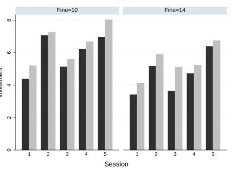
Figure 1 provides a first picture of average decisions in each treatment. The histogram corresponds to the average number of tokens invested in the risky activity in each of the five sessions and for the two levels of the fine (either low, set equal to 10, or high, to 14). The comparison between the two sides of
5
Figure 1: Average investment in the risky activity 0 2 4 6 8 1 2 3 4 5 1 2 3 4 5 Fine=10 Fine=14 Investment Session
Legend. Dark bars: Individual Lottery ; Grey bars: Designation.
Note. Average number of tokens invested in the risky activity in each treatment, by session.
Figure 1 clearly shows that the investment in the risky activity is higher when the fine is low, indicating a negative impact of the fine on risky behavior. This disciplining effect of the fine is particularly noticeable in our set of sessions, since the order of the two levels of fine is randomized across the 44 periods of each session.
If we consider the overall statistics in Figure 1, the comparison of the investment gap between the two treatments (for each paired dark and gray bars) keeps the same sign: the average number of tokens invested in the risky activity is higher under Designation than under Individual Lottery, whatever the session and the level of the fine. In other words, the set of participants seems to perceive a lower level of risk in treatment Designation.
This preliminary evidence is concordant with our hypothesis that the wording used in Designation affects the perceived probability of being monitored. Since we do not elicit the actual believes in the experimental design,6 this is however unobservable unless investment behavior do is sensitive to the perceived decision context. Beyond the existing experimental literature on decision making, evidence on that point can be derived from behavior inside each treatment.
6
Examples of such procedures include Holt (1986); Karni (1999); Nyarko and Schotter (2002). We deliberately ruled out this design to avoid artificially focusing attention of the subjects on correct forecasts of the probabilities at stake, rather than on decision making.
Table 1: Mean investment in the risky option
Risk aversion index 1 2 3 4 5 6 7 8 9 Overall
Number of people 1 1 6 14 14 27 21 6 10 100 Investment F = 10 mean 9.55 6.64 7.79 9.05 7.81 6.79 4.32 2.32 0.80 5.95 under (st. dev.) (4.93) (4.46) (8.79) (8.07) (7.27) (6.45) (5.82) (5.61) (2.51) (6.97) Individual F = 14 mean 10.27 6.73 6.00 6.24 6.99 5.72 2.76 2.14 0.25 4.66 Lottery (st. dev.) (3.17) (5.20) (8.45) (7.60) (7.16) (6.32) (4.77) (5.14) (1.37) (6.48) Investment F = 10 mean 11.27 9.82 6.36 9.62 8.62 7.71 5.31 2.23 0.75 6.55 under (st. dev.) (4.54) (3.22) (8.04) (8.38) (7.36) (6.78) (6.17) (5.28) (2.70) (7.18) Designation F = 14 mean 12.09 7.82 5.74 7.73 7.08 6.48 4.36 1.74 0.29 5.42 (st. dev.) (3.62) (4.51) (8.46) (7.97) (7.45) (6.73) (6.08) (4.79) (1.28) (6.94) Note. The first raw provides the number of individuals for whom the risk aversion index derived from Part 1 of the experiment is the one indicated in column. The last four raws describe the average investment (chosen between 0 and 20) – and the corresponding standard deviations in parenthesis – in the risky lottery in both treatments – Individual Lottery and Designation – and for the two levels of the fine considered.
4.1 Investment decision under risk
A first investigation into the investment behavior in each treatment is provided in Table 1. In this table, we rank participants according to the risk aversion index measured in the first part of the experiment. The shape of the distribution of the 100 participants according to this risk aversion index is quite similar to the standard results given by Holt and Laury (2002, 2005) although our panel is slightly more risk averse. While in the study by Holt and Laury (2002) most of the distribution can be found for the index levels between 4 and 6, in our experiment the corresponding range is between 4 and 7, in which 76% of the participants fall. The queues of the distribution are very thin, especially for lower values of the index with only one person being measured at 1 and 2.
In the bottom part of Table 1, we calculate the mean investment in the risky option among the group of participants with the same risk aversion index, by treatment and levels of the fine. One should note that such aggregate comparisons in the quantities invested in the risky lottery make sense in our experiment because each participant overall faces the same set of probabilities (from 0.05 to 0.55).
If we focus the analysis on the most representative risk aversion indexes (i.e between 4 and 7) a higher level of fine or a higher level of risk aversion clearly decreases the investment in the risky activity. Consequently, the gap observed above between the two treatments is not contradictory with the co-existence of a disciplining effect of the fine and the standard effect of risk aversion on the level of the risky activity.
We statistically check the sensitivity of investment behavior to the perceived environment through random effect Tobit models where the endogenous variable is the number of tokens invested in the risky activity under Individual Lottery (Table 2.a) and under Designation (Table 2.b).
All econometric estimates go in the expected direction regarding the impact of the level of the fine, the attitude toward risk and the probability of being detected on investment in the risky activity. The disciplining effect of all three variables is strongly significant. Investment behavior hence unambiguously reacts to the environment, as perceived by the participants. This allows us to assess the relevance of comparative optimism when incentives are at stake.
4.2 Optimism with incentives
Our measure of optimism derives from the comparison of the number of tokens invested in the risky activity between the two treatments. Indeed, one should expect the same level of investment from perfectly rational players for a given fine and a given probability of monitoring. This does not rule out choice errors, however, particularly in our experimental setting.
Since each participant has to sequentially choose a level of risky investment for two sets of twenty-two periods (with randomized pairs of fine and probability), we can expect a (small) error margin between the two treatments even from rational participants. As suggested by the rather large standard errors provided in Table 1, this indeed seems to be at stake even in individual behavior. However note that such a noisy behavior would on aggregate imply investment differences between the two treatments to be symmetrically distributed around zero. If we observe a persistent and significant difference (with the same sign) among the hundred participants, the error shifts into a bias. As a result, a significant increase in the number of invested tokens in the risky activity under Designation as compared to the level chosen under Individual Lottery (for the same level of the fine and the same probability of monitoring) uncovers a comparative optimism bias: the context between the two treatments is perceived as being so different that it is more likely to escape the control when the risk is defined by the mechanism used under Designation.
Table 3 presents the distribution of mean investment variations according to the risk aversion index. The upper part of the table displays absolute variations measured as the ratio of investment variations between treatments to the total number of available tokens in each period (equal to 20). With a few exceptions, the variation is positive and ranges from a small difference to more than a 10% increase in the tokens allocated to the risky lottery under Designation. For the risk aversion index from 4 to 7, in particular, the mean investment variations are all positive and in favor of a comparative optimism bias, whatever the level of the fine. The bottom part of Table 3 repeats the same information but in relative terms, in the sense that the variation is divided by the investment under Individual Lottery. The picture is a rather strong impact of the wording used in Designation, inducing an average increase of 37% in the number of tokens invested.
The observed differences are statistically assessed using non-parametric tests on investment changes between treatments. Table 4 provides statistics and parameters from Wilcoxon signed rank test. The
Table 2: Tobit regressions on investment decisions in each treatment Table 2.a Individual Lottery Table 2.b Designation
Coef. Stud. t Coef. Stud. t Fine -0.68∗∗∗ -7.82 Fine -0.55∗∗∗ -6.97 Risk aversion index -3.41∗∗∗ -12.01 Risk aversion index -3.52∗∗∗ -13.54 Probability -43.42∗∗∗ -34.43 Probability -45.84∗∗∗ -40.67 Log-Likelihood -4007.41 Log-Likelihood -4064.31
Significance levels: ∗∗∗ 10%,∗∗5%,∗∗∗1%.
Note. Individual random effects Tobit. Endogenous variable: number of tokens invested in the risky option under Individual Lottery (Table 2.a) and Designation (Table 2.b). The following individual covariates are included in the regression but not reported here: age, gender, marital status, number of children, employment and individual’s diploma as well as mother’s diploma and father’s diploma.
Table 3: Mean investment variations induced by Designation (in %)
Risk aversion index 1 2 3 4 5 6 7 8 9 Overall
F = 10 8.6 15.9 -7.1 2.9 4.1 4.6 4.9 -0.5 -0.3 3.0 Mean (st. dev.) (32.6) (18.3) (24.1) (30.1) (32.1) (27.1) (23.2) (15.0) (9.2) (25.7) F = 14 9.1 5.5 -1.3 7.4 0.5 3.8 8.0 -2.0 0.2 3.8 (st. dev.) (22.7) (28.2) (29.5) (35.4) (29.6) (26.7) (22.0) (15.4) (5.1) (26.1) variation Overall 8.9 10.7 -4.2 5.2 2.3 4.2 6.5 -1.2 0.0 3.4 (st. dev.) (27.4) (23.8) (27.0) (32.9) (30.9) (26.9) (22.6) (15.2) (7.4) (25.9) Mean F = 10 87.8 155.9 -18.4 8.4 27.2 40.0 43.4 0.6 21.2 31.1 (st. dev.) (231.4) (370.0) (60.9) (70.6) (166.9) (149.9) (148.3) (80.2) (101.3) (145.3) relative F = 14 30.5 37.2 -13.6 32.5 25.7 49.4 98.7 -14.6 31.4 45.5 (st. dev.) (64.8) (107.7) (52.5) (217.8) (111.8) (151.3) (250.3) (79.5) (103.7) (173.9) variation Overall 59.1 96.6 -16.3 18.9 26.5 44.5 68.0 -7.0 24.6 37.7 (st. dev.) (168.4) (272.1) (57.1) (153.5) (142.6) (150.5) (201.7) (78.8) (99.6) (159.3) Note. Each cell provides the investment variation between Individual Lottery and Designation averaged across individuals for whom the measured risk aversion index in the one provided in column. The average variation reported in the first three rows is the absolute variation (i.e. invested quantities under Designation minus invested quantities under Individual Lottery) in percentage of the number of available tokens, differentiated according to the level of the fine. The average variation reported in the last three rows is the relative variation in % (i.e. ratio of absolute variation to invested quantities under Individual Lottery), differentiated according to the level of the fine.
null hypothesis is unchanged investment decision between the two treatments. Whatever the level of the fine, comparative optimism is overall confirmed with a strong confidence level (p-value smaller than 1%). The desagregation according to the risk aversion index seems to be mainly driven by the number of observations. Except for a risk aversion index equal to 5, we confirm the existence of a comparative optimism bias for the range 4 to 7, gathering the most part of the participants.
5
Conclusion
This paper introduces an experimental test of comparative optimism, in which mis-perception has finan-cial consequences. Optimism is identified thanks to sequential investment decisions into two lotteries. The first one gives rise to a constant return, while the other one randomly leads with known probability to either a higher or a lower return. For each individual, investment decisions are observed twice for 22 return–probability parameter combinations. The only difference between the two decision contexts is the way the probability of a low return is worded. It is highlighted as an individual variable in the Individual Lottery treatment, while explicit reference to the whole group is used in the treatment called Designa-tion. Except for this dimension, the environments are two-by-two identical, including the risk faced during the decision. For given parameters, variations in the investment hence reveal mis-perceptions of the relative probability of experiencing the low return.
Observed behavior in the experiments provide a clear support to comparative optimism bias. Un-derlying the collective dimension of the probability induces an average 35% relative increase in the investment in the risky lottery. Subjects hence exibit a strong tendency to under-evaluate their own likelihood of experiencing an unfavorable event as compared to the one of others. This evidence is in accordance with earlier results in psychology. A risk aversion index is produced in the experiment using a standard procedure borrowed to Holt and Laury (2002, 2005). This allows us to assess the link between the two behavioral motives. No clear pattern arises linking comparative optimism bias and risk aversion.
Table 4: Non parametric tests on investment variations
Risk Aversion Index 1 2 3 4 5 6 7 8 9 Overall
Number of Negative 3 1 19 34 47 77 44 6 5 236 observed Zero 1 1 40 80 51 90 104 53 99 519 F = 10 differences Positive 7 9 7 40 56 130 83 7 6 345 Test z 0.891 2.595 -2.498 0.862 1.306 3.827 3.309 0.295 0.284 4.611 p-value 0.373 0.009 0.012 0.389 0.192 0.000 0.001 0.768 0.776 0.000 Number of Negative 5 5 9 31 40 70 25 8 2 195 observed Zero 1 0 50 74 62 102 121 53 103 566 F = 14 differences Positive 5 6 7 49 52 125 85 5 5 339 Test z 0.759 0.584 -0.486 2.157 1.043 3.820 5.833 -0.826 1.130 6.200 p-value 0.448 0.559 0.627 0.031 0.297 0.000 0.000 0.409 0.258 0.000 Number of Negative 8 6 28 65 87 147 69 14 7 684 observed Zero 2 1 90 154 113 192 225 106 202 1085 Overall differences Positive 12 15 14 89 108 255 168 12 11 431 Test z 1.286 1.991 -2.223 2.144 1.636 5.386 6.373 -0.378 0.927 -7.608 p-value 0.198 0.046 0.026 0.032 0.102 0.000 0.000 0.705 0.354 0.000 Note. Statistics and parameters from the Wilcoxon signed rank test of unchanged investment between Individual Lottery and Designation for those individuals whom measured risk aversion index is the one indicated in column. In each part, the first three raws report the number of positive, zero and negative differences. The last two raws provide the test statistic and the p-value on error associated with rejection of unchanged investment hypothesis. Upper part: low level of fine; Middle part: high level fine ; Upper part all parameters.
In doing so, we introduce a new experimental design with the attractive feature of measuring opti-mism bias for a given risk environment. Some robustness test still has to be performed. First, our results show that optimism supports a distortion of probabilities. In line with earlier results on this subject (Kahneman and Tversky, 1979; Tversky and Wakker, 1995), a proper consideration of this aspect would require to measure optimism on the whole range of probabilities, rather than up to 0.55 only. Second, some unwarranted changes in behavior could be induced by the variation in the space of possible events between treatments – 100 under Individual Lottery, 20 under Designation. A purer setting would de-scribe Individual Lottery within a 20 possible events range. Although this kind of “scale effect” must be of second order, some robustness check have to be performed. Further researches based on our protocol will primarily focus on these both developments.
Should our result be robust to this further developments, it highlights a deep impact on behavior of the way monitoring is publicly displayed. The most diffuse and anonymous the set out is, the less optimistic criminals would be. Through optimism, communication hence appears as a mean to strengthen monitoring at virtually no cost. A fine tuning of policies based on this device requires further investigations into the individual determinants of replies to such frame variations.
References
Alicke, M. (1985). Global self-evaluation as determined by the desirability and controllability of trait adjectives. Journal of Personality and Social Psychology 49 (6), 1621–1630.
Becker, G. S. (1968). Crime and punishment: An economic approach. Journal of Political Economy 76 (2), 169–217.
Bosch-Domènech, A., Silvestre, J. (2006). Risk aversion and embedding bias. Universitat Pompeu Fabra Working Paper (934).
Camerer, C., Lovallo, D. (1999). Overconfidence and excess entry: An experimental approach. American Economic Review 89 (1), 306–318.
Clark, J., Friesen, L. (2006). Overconfidence in forecasts of own performance: An experimental study. University of Canterbury Working paper 06 (09).
Das, M., van Soest, A. (1999). A panel data model for subjective information on household income growth. Journal of Economic Behavior and Organization 40 (4), 409–426.
Dominitz, J., Manski, C. F. (1997). Using expectations data to study subjective income expectations. Journal of the American Statistical Association 92 (439), 855–867.
Fischhoff, B., Parker, A. M., Bruin, W. D., Downs, J., Palmgren, C., Dawes, R., Manski, C. F. (2000). Teen expectations for significant life events. The Public Opinion Quarterly 64 (2), 189–205.
Harrison, G. W., Johnson, E., McInnes, M. M., Rutström, E. E. (2005). Risk aversion and incentive effects: Comment. American Economic Review 95 (3), 897–901.
Hoelzl, E., Rustichini, A. (2005). Overconfident: Do you put your money on it? Economic Journal 115 (503), 305–318.
Holt, C. A. (1986). Scoring-rule procedures for eliciting subjective probability and utility functions. In: Goel, P. K., Zellner, A. (Eds.), Bayesian Inference and Decision Techniques: Essays in Honor of Bruno de Finetti. North Holland Press, Amsterdam.
Holt, C. A., Laury, S. K. (2002). Risk aversion and incentive effects. American Economic Review 92 (5), 1644–1655.
Holt, C. A., Laury, S. K. (2005). Risk aversion and incentive effects: New data without order effects. American Economic Review 95 (3), 902–904.
Kahneman, D., Tversky, A. (1979). Prospect theory: An analysis of decision under risk. Econometrica 47 (2), 263–292.
Karni, E. (1999). Elicitation of subjective probabilities when preferences are state-dependent. Interna-tional Economic Review 40 (2), 479–486.
Nyarko, Y., Schotter, A. (2002). An experimental study of belief learning using elicited beliefs. Econo-metrica 70 (3), 971–1005.
Park, Y.-J., Santos-Pinto, L. (2006). Forecasts of relative performance in tournaments: Evidence from the field. Working Paper .
Scheier, M. F., Carver, C. S., Bridges, M. W. (1994). Distinguishing optimism from neuroticism (and trait anxiety, self-mastery, and self-esteem): A re-evaluation of the life orientation test. Journal of Personality and Social Psychology 67, 1063–1078.
Tversky, A., Wakker, P. (1995). Risk attitudes and decision weights. Econometrica 63 (6), 1255–1280. Weinstein (1980). Unrealistic optimism about future life events. Journal of Personality and Social
Psy-chology 39 (5), 806–820.
Zeiliger, R. (2000). A presentation of regate, internet based software for experimental economics. http://www.gate.cnrs.fr/ zeiliger/regate/RegateIntro.ppt, GATE .
Appendix A
Risk aversion inference from Holt and Laury’s test
Each period involves a decision between two lotteries (options): “Option A” and “Option B”. The high (low) payoffs are respectively 200ecu (160ecu) and 385ecu (10ecu). Over the ten choice periods, the probability of an high payoff in each Option is sequentially increased from 1/10 to 10/10, by increments of 1/10. As in Holt and Laury (2002), the ten lottery-couples are proposed in increasing order.
Assuming the following CRRA utility function: u(x) = x1−r, x > 0, the relative risk aversion
parameter, r, can be inferred from the observed sequence of choices according to the following table:
Observed choices r Observed choices r
A,A,A,A,A,A,A,A,A,B r > 1.37 A,A,A,A,B,B,B,B,B,B −0.15 < r < 0.15
A,A,A,A,A,A,A,A,B,B 0.97 < r < 1.37 A,A,A,B,B,B,B,B,B,B −0.49 < r < −0.15 A,A,A,A,A,A,A,B,B,B 0.68 < r < 0.97 A,A,B,B,B,B,B,B,B,B −0.95 < r < −0.49 A,A,A,A,A,A,B,B,B,B 0.41 < r < 0.68 A,B,B,B,B,B,B,B,B,B r < −0.95 A,A,A,A,A,B,B,B,B,B 0.15 < r < 0.41
Appendix B
Instructions for treatment “Designation”
You are involved in an experiment part of a scientific research program supported by both National Agency of Social Security Organisms (ACOSS) and National Center of Scientific Research (CNRS). During this experiment, you will earn some money. Your monetary payoff depends on your decisions. Timing of the experiment:
The experiment includes three parts.
The first part consists in 10 rounds and the two others in 22 rounds each, then 54 rounds in all. In each round you make one decision, meaning that you make 54 decisions during this experimental session. Among your 54 decisions, only one determines your final monetary payoff, the one which is selected by the draw performed at the end of the experiment.
In each round, you obtain a score for your decision. Your scores are measured in ecu (Experimental Currency Unit ). Your score in each round is revealed to you only at the end of the experiment, as a summary table. Your final earning is equal to your score during the round drawn at the end of the
experiment. Like your scores, your final earning is measured in ecu. At the end of the experiment, your final earning is converted into Euro.
[Instructions for the first part are inserted here.]
Calculation of your final earning in ecu and its value in Euro:
Among the 54 decisions you made during the three parts of the experimentation, only one determines your final earning.
For each participant, we select one decision using a draw performed at the end of the experiment. This final draw is performed in a ballot box containing 54 balls numbered from 1 to 54. The number of the drawn ball determines the round taken into account in the calculation of your final earning. You don’t know in advance which decision will determine your final earning.
Your final earning is equal to your score during the round drawn at the end of the experiment. Your scores and your final earnings are measured in ecu. At the end of the experiment, your final earning in ecu will be converted according to the following rate: 30 ecu = 1 euro.
On top of this, a 7 euros show-up fee is added. This sum will be paid cash individually and privately before you leave the laboratory. Whatever your final earnings, you cannot lose money.
[The first part is played. Instructions for the subsequent part are then distributed and read aloud.] Timing of the third (second) part
[The alternative instructions for Individual Lottery are provided in brackets] This part involves 22 rounds, each one including one decision.
Timing of a round:
Each round includes two steps.
At the beginning of each round, you receive 20 tokens and your decision consists in allocating all your tokens between 2 options: option A and option B. At each round, the two options will appear on your screen and you will choose the allocation of your tokens by scrolling on a scale from 0 to 20. When you scroll right or left, the number of tokens allocated to each option appears below the scale. Once your choice is made, click on the button labeled ”OK”.
At the end of each round, we designate randomly n individuals out of the 20 participants seat in the room. We don’t tell you whether you are designated or not. [Individual Lottery: At the end of each round, we draw lots for a ball, for each participant, in an individual ballot box. Each ballot box contains 100 balls, split in p black balls and 100-p white balls. Each participant has thus p chances out of 100 for the drawn ball to be black and (100-p) chances out of 100 for it to be white. We don’t tell you the result of the draw.]
How is your score calculated in each round:
Your score in each round is equal to the sum of earnings from tokens allocated to option A and earnings from tokens allocated to option B.
Calculation of earnings from tokens allocated to option A:
Whether you are designated or not [Individual Lottery: whatever the colour of the ball drawn]: Each token brings you in 15 ecu.
These earnings are random and depend on whether you have been designated or not [Individual Lottery: depend on the colour of the ball drawn].
If you have not been designated [Individual Lottery: If the drawn ball is white]: Each token brings you in 20 ecu.
If you are designated [Individual Lottery: If the ball drawn is black ]: Each token brings you in (15-F) ecu. The number of individual designated among the 20 participants [Individual Lottery: the number of black balls in the Individual Lottery] and the value of F appear on the screen at the beginning of each round, before you allocate your tokens between the 2 options.
At the end of each round, we don’t tell you neither if you have been designated [Individual Lottery: neither the colour of the ball drawn] nor your score. Having been designated [Individual Lottery: the colour of the ball drawn] and your score in each round are revealed to you only at the end of the experimental session in a summary table.
We remind you that in this experimental session only one of your scores determines your final monetary payoff; the one corresponding to the round picked out by the final draw.
****** Example 1:
We tell you that:
- We designate 6 individuals out of 20 participants (Individual Lottery: you have 30 chances out of 100 for the ball drawn to be black, i.e. the value of p is 30 )
- The value of F is 5
• If you allocate your 20 tokens to option A:
– Whether you are designated or not (Individual Lottery: whatever the colour of the drawn ball is), your score in this round is: 20*15 = 300 ecu.
• If you allocate your 20 tokens to option B:
– If you are not designated [Individual Lottery: If the ball drawn is white], your score in this round is: 20*20 = 400 ecu.
– If you are designated [Individual Lottery: If the ball drawn is black ], your score in this round is: 20*(15-5) = 200 ecu.
• If you allocate 10 tokens to option A and 10 tokens to option B:
– If you are not designated [Individual Lottery: If the ball drawn is white], your score in this round is: 10*15 + 10*20 = 350 ecu.
– If you are designated [Individual Lottery: If the ball drawn is black ], your score in this round is: 10*15 + 10*(15-5) = 250 ecu.
****** Example 2:
We tell you that:
- We designate 1 individual out of 20 participants [Individual Lottery: you have 5 chances out of 100 for the drawn ball to be black, i.e. the value of p is 5 ]
- The value of F is 10
• If you allocate your 20 tokens to option A:
– Whether you are designated or not [Individual Lottery: whatever the colour of the ball drawn is], your score in this round is: 20*15 = 300 ecu.
• If you allocate your 20 tokens to option B:
– If you are not designated [Individual Lottery: If the ball drawn is white], your score in this round is: 20*20 = 400 ecu.
– If you are designated [Individual Lottery: If the drawn ball is black ], your score in this round is: 20*(15-10) = 100 ecu.
• If you allocate 5 tokens to option A and 15 tokens to option B:
– If you are not designated [Individual Lottery: If the ball drawn is white], your score in this round is: 5*15 + 15*20 = 375 ecu.
– If you are designated [Individual Lottery: If the ball drawn is black ], your score in this round is:5*15 + 15*(15-10) = 150 ecu.