HAL Id: inria-00204481
https://hal.inria.fr/inria-00204481
Submitted on 27 Mar 2009
HAL is a multi-disciplinary open access
archive for the deposit and dissemination of
sci-entific research documents, whether they are
pub-lished or not. The documents may come from
teaching and research institutions in France or
abroad, or from public or private research centers.
L’archive ouverte pluridisciplinaire HAL, est
destinée au dépôt et à la diffusion de documents
scientifiques de niveau recherche, publiés ou non,
émanant des établissements d’enseignement et de
recherche français ou étrangers, des laboratoires
publics ou privés.
Time Modeling in MARTE
Charles André, Frédéric Mallet, Robert de Simone
To cite this version:
Charles André, Frédéric Mallet, Robert de Simone. Time Modeling in MARTE. ECSI Forum on
specification & Design Languages (FDL), ECSI, Sep 2007, Barcelona, Spain. pp.268-273.
�inria-00204481�
Time modeling in MARTE
Charles Andr´e, Fr´ed´eric Mallet, Robert de Simone
I3S, Universit´e de Nice-Sophia Antipolis, CNRS, F-06903 Sophia Antipolis
Aoste Project, I3S/INRIA
E-mail:
{
candre,fmallet,rs
}
@sophia.inria.fr
Abstract
This article introduces the Time Model subprofile of MARTE, a new OMG UML Profile dedicated to Modeling and Analysis of Real-Time and Embedded systems. After a brief presentation of former time modeling elements present in SPT and UML2, we introduce the Time meta-model of MARTE. It defines physical and logical time, timed model elements and their associated properties. We present both the time domain view and the UML representation of the most important concepts. Various time bases (called clocks in the profile) can be correlated using clock relations and constraints, built from a core set predefined in the profile. Constraints are usually collected from scheduling and partitioning decisions taken in the course of design flow for embedded systems. We illustrate this on two simple examples.
I. Introduction
Modeling of Time should certainly be a central con-cern in Model-Driven Engineering dedicated to Real-Time Embedded Systems (RTES). Real-Timed extensions should allow to support a rich design flow, that can encompass both established and emerging new tech-niques for model-based optimization, transformation and analysis of systems. Indeed, embedded system mod-els very often consists of a predefined set of appli-cation functions, and of execution platforms on which to allocate these functions. Application elements are increasingly componentized, may coexist and possibly cooperate concurrently. Execution platforms increasingly comprise parallel resources for both communications and computations.
The design challenge in embedded system modeling is then to provide model-level compilation techniques that provide support for both spatial distribution and temporal scheduling of applications onto platforms (collectively called allocation). This approach is therefore akin to system level design techniques such as advocated in SysML [1]. But SysML, just like UML, hardly formalizes
its real-time aspects.
This global issue triggered over the years a number of proposals for specific representation formalisms, and their associated particular design techniques. These mod-els then can be, and often have been, represented inside the scope of the UML [2], [3], [4], [5], [6]. But this is typically done, a) mostly at the metamodel level, and b) without any clear interpretation of any kind of the time annotations in the framework of the UML. This raises the risk of mismatch between the private interpretation inherited from the formalism and the existing UML semantics [7].
The primary objective of the Time subprofile in MARTE [8] was to provide basic and advanced time modeling concepts, with interpretation inside the UML modeling level, not outside. These time-related concepts could then be used to build various Models of Com-putation and Communication (MoCC). Importantly, the profile should subsume the former SPT [9] and the UML2 Simple Time models [10], while extending them towards the possibility of modeling much richer MoCC-based design approaches [11], [12], [13], [14].
Time as considered in design can be of physical or logical nature. Physical time is continuous, but can usu-ally be discretized into chronometric clocks under appro-priate assumptions. Logical time is less often recognized in itselft as an explicit modeling concept. Processings and execution steps performed at the rate of a processor cycle (which may vary according to power consumption management), or triggered by successive occurrences of an external event (such as completion of an engine revolution) are simple example of that. Often the allo-cation process may be perceived as this : asynchronous concurrent application components are each considered as being governed by their own (local) logical clock, connected to appropriate events; then the allocation itself consists in fitting these various clock threads onto a single (or at least more correlated) synchronous clock, subject to constraints of various sources abstracted from physical time properties and requirements. The transformation and analysis steps involved in the proper mapping are (at least implicitly) dealing with scheduling objects that are
relations between logical and physical clocks attached to the various processings. MARTE Time profile is meant exactly to represent that.
In the sequel, we shall describe the profile in greater details and its position with respect to other parts of MARTE. We start with the domain view and give an overview of the UML representation. Two examples illustrate the usage of the profile.
II. Time domain view
This section describes the MARTE Time domain view, i.e., the main concepts related to time and their relation-ships. In an MDE approach, this is done through meta-modeling. Before reviewing the MARTE Time models, we will have a look at the former UML profile for Time: SPT
A. SPT
The UML Profile for Schedulability, Performance, and Time (SPT) aimed at filling the lacks of UML 1.4 in some key areas that are of particular concern to real-time system designers and developers. SPT introduces a quantifiable notion of time and resources. It annotates model elements with quantitative information related to time, information used for timeliness, performance, and schedulability analyses.
SPT only considers (chrono)metric time, which makes implicit reference to physical time. It provides time-related concepts: concepts of instant and duration, con-cepts for modeling events in time and time-related stim-uli. SPT also addresses modeling of timing mechanisms (clocks, timers), and timing services. SPT, which relies on UML 1.4, had to be aligned with UML 2.1. This is one of the objectives of the MARTE profile, presented below.
UML 2 has included a new package called
Simple-Time, part of the CommonBehaviorpackage. The main
new meta-classes are TimeEventandObservation(Time
and Duration). The model is kept very simple and is intended to be extended in specialized profiles. This is the specific agenda of MARTE Time model.
B. MARTE time model
As a successor of SPT, MARTE has to support a metric time with implicit reference to physical time. However, MARTE goes beyond this quantitative model of time and adopts more general time models suitable for system design. In MARTE, Time can be physical, and considered as dense or discretized, but it can also be logical, and related to user-defined clocks. Time may even be multiform, allowing different times to progress in a non-uniform fashion, and possibly independently to any (direct) reference to physical time.
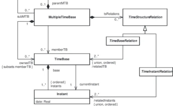
1) Concept of time structure: The building element in a time structure is the TimeBase (Fig. 1). A time base is a totally ordered set of instants. A set of instants can be
MultipleTimeBase TimeBase date: Real Instant { ordered } instants base 1 1..* memberTB 0..* TimeStructureRelation tsRelations 0..* currentInstant 1 TimeBaseRelation TimeInstantRelation 2..* /relatedInstants { union, ordered } 0..* 0..1 parentMTB subMTB 0..* 1 ownedTB { subsets memberTB } 2..* { union, ordered } /relatedTB
Fig. 1. Time structure (Domain view).
discrete or dense. The linear vision of time represented by a single time base is not sufficient for most of the applications, especially in the case of multithreaded or distributed applications. Multiple time bases are then
used. AMultipleTimeBaseconsists of one or many time
bases. A time structure contains a tree of multiple time bases.
Time bases are a priori independent. They become dependent when instants from different time bases are linked by relationships (coincidence or precedence). The
abstract class TimeInstantRelationin Fig. 1 has
Coinci-denceRelationandPrecedenceRelationas concrete
sub-classes. Instead of imposing local dependencies between instants, dependencies can be directly imposed between
time bases. ATimeBaseRelation(or more precisely one
of its concrete subclasses) specifies many (possibly an infinity of) individual time instant relations. This will
be illustrated later on some time base relations.
Time-BaseRelation and TimeInstantRelation have a common
generalization: the abstract classTimeStructureRelation.
As a result of adding time structure relations to multiple time bases, time bases are no longer independent and the instants are partially ordered. This partial ordering of in-stants characterizes the time structure of the application. This model of time is sufficient to check the logical correctness of the application. Quantitative information, attached to the instants, can be added to this structure when quantitative analyses become necessary (see be-low).
2) Access to time: In real world technical systems, special devices, called clocks, are used to measure the progress of physical time. In MARTE, we adopt a more general point of view: a clock is a model element giving access to the time structure. Time may be logical or physical or both.
A Clock makes reference to a TimeBase (Fig. 2), and
thus indirectly to the instants of this timebase. Thenature
attribute indicates whether the accessed time is dense or
discrete. A Clock accepts units (acceptedUnitsproperty).
Unitis a concept introduced in the MARTE NFP
(Non-functional property) domain view. One of these accepted units is the defaultUnit. A clock may own an event
TimeBase nature: TimeNatureKind resolution: Real=1.0 origin: Real [0..1] currentTime: Real maximalValue: Real[0..1] Clock 1 timeBase Event Unit 0..1 0..1 clockTick acceptedUnits 1..* defaultUnit {subsets acceptedUnits} 1 Fig. 2. Clock
(clockTick). This event occurs at each change of the
current time of the clock. Other attributes characterize quantitive information that can be attached to a clock.
The resolutionproperty specifies the readout granularity
of the clock, expressed in defaultUnit unit. Its default
value is 1.0. The optional attribute origin specifies the
possible offset in the clock reading. The optional attribute
maximalValue expresses the limited capability of usual
clocks to represent arbitrary large instant values: the clock “rolls over” when the currentTime value gets at the maximal value. For instance, for a discrete periodic
clock, the time value attached to the kth instant is given
by(origin+(k−1)∗resolution) mod maximalV alue.
Clock LogicalClock Event definingEvent 0..1 standard: TimeStandardKind [0..1] stability : Real [0..1] offset: DurationValue [0..1] skew: Real [0..1] drift: Real [0..1] ChronometricClock PhysicalTime 0..1 referenceClock
Fig. 3. Logical and chronometric clock
Clockis an abstract concept. There exist two concrete
specializations ofClock:LogicalClockand
Chronometric-Clock. A chronometric clock is a clock making
refer-ence to physical time. A special attention is then put on the quantitative information attached to this model. Non functional properties like stability, skew, etc can
be defined for these clocks with respect to some
refer-enceClock. On the other hand, a logical clock can be
defined by any event (definingEvent property); in this
case, the clock ticks at each occurrence of the defining event. Logical time is usually counted in the number of
ticks. So,tickis a predefined unit often used as the default
unit for a logical clock.
3) Time value specifications: An application may use time in two ways: either as a reference to a time instant or as a time span. So, MARTE introduces two distinct
concepts:InstantValueandDurationValue, specializations
of the abstract concept of TimeValue. Since the access
to time is done through clocks, aTimeValuerefers to a
Clock(theonClockproperty). A time value also have an
associated unit. When optional propertyunitis given, it
must be used instead of default unit of the associated clock. The attribute nature specifies whether the time values associated with the clock take their values in a dense or discrete domain.
Clock Instant 0..* InstantValue denotedInstant TimeInterval 0..* denotedTimeInterval nature: TimeNatureKind TimeValue isMinOpen: Boolean [1] isMaxOpen: Boolean [1] TimeIntervalValue min 1 max 1 Unit unit 0..1 1 onClock lower 1 upper 1 DurationValue intervalValue 1
Fig. 4. Time values
4) Time-related concepts: A timed element is a most general concept. TimedElement is an abstract class gen-eralization of all other timed concepts. It associates a non empty set of clocks with a model element. The semantics of the association with clocks depends on the kind of timed element. Clock TimedElement 1..* on ModelElement
Fig. 5. Timed element
Events and behaviors can be directly bound to time. The occurrences of a (timed) event refer to points of time (instants). The executions of a (timed) behavior refer to points of time (start and finish instants) or to segments of time (duration of the execution).
TimedEvent(TimedProcessing, resp.) is a concept
rep-resenting an event (a processing, resp.) explicitly bound to time through a clock. In this way, time is not a mere annotation: it changes the semantics of the timed model elements.
Other timed elements—not detailled in this
presentation—are also defined in the MARTE Time domain: timed observations, and timed constraints. As timed elements they explicitly bind observations or constraints to clocks.
III. UML view of Time in MARTE
A. The Time sub-profileThe time structure presented above constitutes the semantic domain of our time model. The UML view is defined in the “MARTE Time profile”. This profile introduces a limited number of powerful stereotypes. We have striven to avoid the multiplication of too specialized
isRelative: Boolean repetition: Integer [0..1] TimedEvent TimedElement every 0..1 when 1 Event TimeValueSpecification DurationValueSpecification
Fig. 6. Timed event
TimedProcessing
0..1 start finish 0..1 0..1 duration
TimedElement TimedBehavior TimedMessage TimedAction
Delay Event DurationValueSpecification CoreElements:: Causality:: CommonBehavior:: Behavior CoreElements:: Causality:: CommonBehavior:: Action CoreElements:: Causality:: Communication:: Request
Fig. 7. Timed processing
stereotypes. Thanks to the sound semantic grounds of our styereotypes, modeling environments may propose patterns for more specific uses.
« stereotype» TimedElement « metaclass » UML::Classes::Kernel::Class nature: TimeNatureKind [1] unitType: Enumeration [0..1] isLogical : Boolean [1] = false resolAttr: Property [0..1] maxValAttr: Property [0..1] offsetAttr: Property [0..1] getTime: Operation [0..1] setTime: Operation [0..1] indexToValue: Operation [0..1] « stereotype» ClockType « metaclass » UML::Classes::Kernel:: InstanceSpecification « stereotype» Clock « stereotype» NFPs::Unit « stereotype» TimedDomain « metaclass » UML::Classes::Kernel:: Package on 1..* unit 0..1 type 1
Fig. 8. MARTE Time profile: Clock.
1) ClockType and Clock: The main sterotypes are
presented in figure 8. ClockType is a stereotype of the
UML Class. Its properties specifies the kind
(chrono-metric or logical) of clock, the nature (dense or discrete) of the represented time, a set of clock properties (e.g., resolution, maximal value. . . ), and a set of accepted time
units. Clock is a sterotype of InstanceSpecification. An
OCL rule imposes to apply theClockstereotype only to
instance specifications of a class stereotyped by
Clock-Type. Theunitof the clock is given when the stereotype
is applied. Unit is defined in the Non Fonctional
Prop-erty modeling (NFPs) subprofile of MARTE; it extends
EnumerationLiteral. It is very convenient because a unit
can be used like any user-defined enumeration literal, and conversion factors between units can be specified (e.g.,
1ms = 10−3s). TimedElement is an abstract stereotype
with no defined metaclass. It stands for model elements which reference clocks. All other timed stereotypes
spe-cializeTimedElement.
2) Clock constraints: ClockConstraintis a stereotype
of the UML Constraint. The clock constraints are used
to specify the time structure relations of a time domain.
The context of the constraint must be aTimedDomain.
The constrained elements are clocks of this timed domain and possibly other objects. The specification of a clock constraint is a set of declarative statements. This raises the question of choosing a language for expressing the clock constraints. A natural language is not sufficiently precise to be a good candidate. UML encourages the use of OCL. However, our clocks usually deal with infinite sets of instants, the relations may use many math-ematical quantifiers, which are not supported by OCL. Additionnally, OCL [15] is made to be evaluatable, while our constraints often have to be processed altogether to get a set of possible solutions. So, we have chosen to define a simple constraint expression language en-dowed with a mathematical semantics. The specification
of a clock constraint is a UML::OpaqueExpression that
makes use of pre-defined (clock) relations, the meaning of which is given in mathematical terms, outside the UML. Our Clock Constraint Specification Language is not normative. Other languages can be used, so long as the semantics of clocks and clock constraints is respected. 3) TimedEvent and TimedProcessing: In UML, an
Event describes a set of possible occurrences; an
oc-currence may trigger effects in the system. A UML2
TimeEvent is an Event that defines a point in time
(instant) when the event occurs. The MARTE stereotype
TimedEventextendsTimeEvent. Its instant specification
explicitly refers to a clock. If the event is recurrent, a repetition period—duration between two successive occurrences of the event—and the number of repetitions may be specified.
In UML, a Behavior describes a set of possible
ex-ecutions; an execution is the performance of an algo-rithm according to a set of rules. MARTE associates a duration, an instant of start, an instant of termination with an execution, these times being read on a clock.
The stereotypeTimedProcessingextends the metaclasses
Behavior,Action, and alsoMessage. The latter extension
assimilates a message tranfer to a communication action.
Note that, StateMachine, Activity, Interaction being
Behavior, they can be stereotyped byTimedProcessing,
B. The Time model library
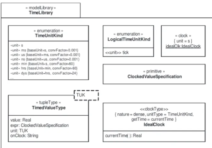
The TimeLibrary (Fig 9) is a user’s model libary that provides enumerations related to time and facilities for using the ideal chronometric time (i.e., the time
referenced in physical laws). TimeUnitKind contains the
main chronometric time units. s (second) is an SI unit. Other units are derived units. All the enumeration literals
are stereotyped byUnit.LogicalTimeUnitKindis a special
enumeration which contains one enumeration literal only.
This literal istick. TheIdealClockand its instanceidealClk
model the abstract and ideal time which is used in
physical laws. It is a dense time. idealClk should be
imported in models that refer to chronometric time.
TimedValueTypeis a templated data type. The template
parameter is an enumeration which contains time units.
« modelLibrary »
TimeLibrary
currentTime( ): Real <<clockType>> { nature = dense, unitType = TimeUnitKind,
getTime = currentTime } IdealClock « clock » { unit = s } idealClk:IdealClock «unit» s
«unit» ms {baseUnit=s, convFactor=0.001} «unit» us {baseUnit=ms, convFactor=0.001} «unit» ns {baseUnit=us, convFactor=0 .001 } «unit» min {baseUnit=s, convFactor=60 } «unit» hrs { baseUnit=min, convFactor=60} «unit» dys {baseUnit=hrs, convFactor=24 } ... « enumeration » TimeUnitKind <<unit>> tick « enumeration » LogicalTimeUnitKind value: Real expr: ClockedValueSpecification unit: TUK onClock: String « tupleType » TimedValueType TUK « primitive » ClockedValueSpecification
Fig. 9. TimeLibrary: a user library for time
Besides libraries, other facilities are offered to MARTE users: concrete languages dedicated to value expressions (Value Specification Language—VSL) and to clock constraint expressions (Clock Constraint Specifica-tion Language—CCSL) [16, Annexes B & C]. The latter defines a core set of constraints that can be extended to express desired relation patterns between timed elements. Examples of such clock constraints are described in a technical report [17]. For lack of room we cannot describe them here. Some constraint relations state that variations in rate or jitter between two clocks are some-how bounded, that clocks are related up to some drift, or that a clock has to be a subclock of some other (with the subclocking mechanism following possibly some pattern). Some relations are more imperative in that they denote the single solution to some clock transformations
(as for instance inb isPeriodicOn a ofPeriod n).
IV. Examples
The first step for the designer is to construct its own, not always perfect, clocks. The first subsection shows how to create chronometric clocks and the second subsection illustrates the use of logical clocks.
A. Chronometric clock specifications
The MARTE TimeLibrary provides a model for the
ideal time used in physical laws:idealClk, which is an
in-stance of the classIdealClock, stereotyped byClockType
(Fig. 10, upper part).idealClk is a dense time clock, its
unit is the SI time units.
currentTime( ): Real resolution: Real {readOnly}
« clockType » { nature = discrete, unitType = TimeUnitKind, resolAttr=resolution, getTime = currentTime }
Chronometric
resolution = 0.01 « clock » { unit = s, standard = UTC }
cc1:Chronometric
resolution = 0.01 « clock » { unit = s, standard = UTC }
cc2:Chronometric
« clockConstraint » { kind = required } { Clock c is idealClk discretizedBy0.001;
cc1 isPeriodicOn c period 10; cc2 isPeriodicOn c period 10; cc1 hasStability 1E-4; cc2 hasStability 1E-4; cc1,cc2 haveOffset [0..5] ms wrt idealClk; } « clock » { unit = s } idealClk:IdealClock currentTime( ): Real « clockType » { nature = dense, unitType = TimeUnitKind,
getTime = currentTime } IdealClock Imported from MARTE::TimeLibrary « TimedDomain » ApplicationTimeDomain
Fig. 10. Chronometric clocks.
After importing the library, new user-defined chrono-metric clocks can be defined. For instance, Fig. 10 defines
the classChronometricwith an attributeresolutionof type
Realand an operationcurrentTimethat allows for reading
the current time. The stereotype ClockType is applied
and the tagged values characterize the nature of clocks represented by this class. Here, the clock is a discrete clock and accepts the units defined by the predefined
EnumerationTimeUnitKind (see Fig. 9). By default, the
clock types are chronometric, not logical.
Actual clocks belong to timed domains, i.e., a package
stereotyped byTimedDomain(Fig. 10, lower part). Here,
a single time domain is considered. It owns three clocks.
idealClk is imported from the library. Two instances of
the class Chronometric,cc1 and cc2, are defined. They
both uses(second) as a time unit and their resolution is
0.01s. The three clocks are a priori independent. A clock
constraint specifies relationships among them. According
to the given constraints, cc1 and cc2 are two 100 Hz
clocks, the stability of which is10−4, and with an offset
less than 5ms.
B. Logical clock specifications
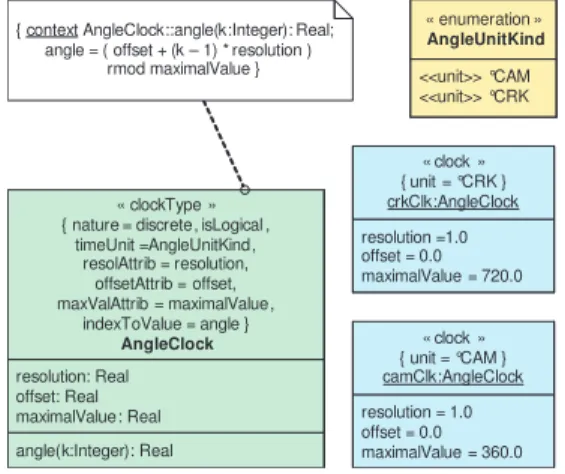
Fig. 11 illustrates the definition of logical clocks. The
discrete, logical, clock type AngleClock is defined. It
has three attributes,resolution,offsetandmaximalValue.
The label function angle associates a real value, the
clock reading, with each instant of the clock. Each instant is uniquely identified by a natural number, its index, inferred from the linear order defined on the clock instants.
The enumerationAngleUnitKinddefines the units,
enu-meration literals stereotyped by NFP::Unit, that can be
used by the clocks.
Two clocks, instances ofAngleClock, are then created.
◦CRK (degree crank), its resolution is 1◦CRK and its
maximal value is720◦CRK, i.e., two revolutions of the
crank shaft. camClkrepresents the camshaft resolutions,
its unit is◦CAM (degree cam), its resolution is1◦CAM
and its maximal value is 360◦CAM , one rotation of
the camshaft. One revolution of the camshaft (mechan-ically) implies two revolutions of the crankshaft, hence
1◦CAM = 2◦CRK. <<unit>> °CAM <<unit>> °CRK « enumeration » AngleUnitKind angle(k:Integer): Real resolution: Real offset: Real maximalValue: Real « clockType » { nature = discrete, isLogical ,
timeUnit =AngleUnitKind, resolAttrib = resolution, offsetAttrib = offset, maxValAttrib = maximalValue, indexToValue = angle } AngleClock resolution =1.0 offset = 0.0 maximalValue = 720.0 « clock » { unit = °CRK } crkClk:AngleClock { context AngleClock::angle(k:Integer): Real;
angle = ( offset + (k – 1) * resolution ) rmod maximalValue } resolution = 1.0 offset = 0.0 maximalValue = 360.0 « clock » { unit = °CAM } camClk:AngleClock
Fig. 11. Logical Clocks.
Fig. 12 uses the clock camClk to represent a
four-stroke engine cycle. This state machine is stereotyped by
TimedProcessing. The on attribute identifies the clock
used and therefore the unit (◦CAM ).
Intake stm « timedProcessing » 4StrokeEngineCycle { on = camClk } Compression Combustion Exhaust after 90 after 90 after 90 after 90
Fig. 12. State machine of a 4-stroke engine cycle.
This example is developed in a previous paper [18] dedicated to the use of multiform time, and the modeling of the “knock control” problem with MARTE.
V. Conclusion
The MARTE Time subprofile provides a limited num-ber of time concepts from which to build Models of Computations with timed interpretations (as examplified by our modeling of AADL aspects in the same pro-ceedings [19]). These concepts rely on the existence of various time threads (or logical clocks) that may drive application elements. Constraint relations may exist be-tween clocks, from the loose asynchronous compositions to stricter simultaneous coincidence. More constraints are raised as result of scheduling decisions, or by abstraction
of timely requirements demanded by the view or im-posed by the execution platform. Solving constraints and committing progressively to particular schedule results from the intended flow of design promoted by MARTE in model-based engineering of embedded systems.
References
[1] OMG, Systems Modeling Language (SysML) Specification, April 2006, OMG document number: ad/2006-03-01. [Online]. Available: http://www.sae.org/technical/standards/AS5506/1 [2] B. Selic, G. Gullekson, and P. Ward, Real-Time Object-Oriented
Modeling. J. Wiley Publ., 1994.
[3] B. P. Douglass, Real-Time UML: developing efficient objects for
embedded systems, ser. Object technology series. Reading, Massachusetts: Addison-Wesley, 1998.
[4] S. G´erard, F. Terrier, and Y. Tanguy, “Using the model paradigm for real-time systems development: Accord/uml,” in
OOIS’02-MDSD, ser. LNCS, vol. 2426. Montpellier (F): Springer-Verlag,
2002.
[5] S. Graf, I. Ober, and I. Ober, “A real-time profile for UML,”
STTT, Software Tools for Technology Transfer, vol. 8, no. 2, pp.
113–127, April 2006.
[6] L. Apvrille, P. Saqui-Sannes, and F. Khendek, “TURTLE-P: a uml profile for the formal validation of critical and distributed systems,” Software and Systems Modeling (SoSyM), vol. 5, no. 4, pp. 449–466, December 2006. [Online]. Available: http://dx.doi.org/10.1007/s10270-006-0029-5
[7] R. De Simone and C. Andr´e, “Towards a “Synchronous Reac-tive” UML profile?” International Journal on Software Tools for
Technology Transfer (STTT), vol. 8, no. 2, pp. 146–155, April
2006.
[8] OMG, UML profile for Modeling and Analysis of Real-Time
and Embedded systems (MARTE), Request for proposals, Object
Management Group, Inc., Needham, MA 02494., February 2005, OMG document number: realtime/2005-02-06.
[9] ——, UML Profile for Schedulability, Performance, and Time
Specification, January 2005, OMG document number:
formal/05-01-02 (v1.1).
[10] ——, UML 2.1 Superstructure Specification, April 2006, OMG document number: ptc/2006-04-02.
[11] E. A. Lee and A. L. Sangiovanni-Vincentelli, “A framework for comparing models of computation,” IEEE Transactions on
Computer-Aided Design of Integrated Circuits and Systems,
vol. 17, no. 12, pp. 1217–1229, December 1998.
[12] J. Buck, S. Ha, E. Lee, and D. Messerschmitt, “Ptolemy: A frame-work for simulating and prototyping heterogeneous systems,”
International Journal of Computer Simulation, special issue on “Simulation Software Development”, vol. 4, pp. 155–182, April
1994.
[13] A. Jantsch, Modeling Embedded Systems and SoCs - Concurrency
and Time in Models of Computation. Morgan Kaufman, 2003. [14] A. Benveniste, B. Caillaud, L. Carloni, P. Caspi, and
A. Sangiovanni-Vincentelli, “Composing heterogeneous reactive systems,” ACM Transactions on Embedded Computing Systems, 2007.
[15] OMG, Object Constraint Language, version 2.0, May 2006, OMG document number: formal/06-05-01.
[16] ——, UML profile for MARTE (2nd rev.), August 2007, OMG document number: still pending.
[17] C. Andr´e, F. Mallet, and R. de Simone, “Modeling time(s) in UML,” Laboratoire I3S - Sophia Antipolis, Tech. Rep., 2007, 24 pages.
[18] C. Andr´e, F. Mallet, and M.-A. Peraldi-Frati, “A multiform time approach to real-time system modeling: Application to an automotive system,” in IEEE 2nd International Symposium on
Industrial Embedded Systems (SIES’2007). IEEE, 2007, pp. 234–
241.
[19] C. Andr´e, F. Mallet, and R. de Simone, “Modeling of immediate vs. delayed data communications: from AADL to UML MARTE,” in ECSI Forum on specification & Design Languages (FDL), September 2007.