HAL Id: hal-02507327
https://hal.archives-ouvertes.fr/hal-02507327v2
Submitted on 28 Oct 2020
HAL is a multi-disciplinary open access
archive for the deposit and dissemination of
sci-entific research documents, whether they are
pub-lished or not. The documents may come from
teaching and research institutions in France or
abroad, or from public or private research centers.
L’archive ouverte pluridisciplinaire HAL, est
destinée au dépôt et à la diffusion de documents
scientifiques de niveau recherche, publiés ou non,
émanant des établissements d’enseignement et de
recherche français ou étrangers, des laboratoires
publics ou privés.
Distributed under a Creative Commons Attribution - NonCommercial - NoDerivatives| 4.0
International License
Comparison of optimal actuation patterns for flagellar
magnetic micro-swimmers
Yacine El Alaoui-Faris, Jean-Baptiste Pomet, Stéphane Régnier, Laetitia
Giraldi
To cite this version:
Yacine El Alaoui-Faris, Jean-Baptiste Pomet, Stéphane Régnier, Laetitia Giraldi. Comparison of
optimal actuation patterns for flagellar magnetic micro-swimmers. IFAC 2020 - 21st IFAC World
Congress, IFAC, Jul 2020, Berlin / Virtual, Germany. �hal-02507327v2�
Comparison of optimal actuation patterns
for flagellar magnetic micro-swimmers
Yacine E. Faris∗,∗∗ Jean-Baptiste Pomet∗St´ephane R´egnier∗∗
Laetitia Giraldi∗
∗Universit´e Cˆote d’Azur, Inria, CNRS, LJAD, McTAO team, Nice,
France.
∗∗Sorbonne Universit´e, CNRS, ISIR, Paris, France
Abstract: In this article, we present a simplified model of a flagellar micro-swimmer actuated by external magnetic fields that is based on shape discretization and an approximation of the hydrodynamical forces. We numerically solve the optimal control problem of finding the actuating magnetic fields that maximizes its horizontal propulsion speed over a fixed time under different constraints on the magnetic field amplitudes and compare the optimal solutions. All the simulated magnetic fields out-perform the standard sinusoidal actuation method that is prevalent in the literature and in experiments. Moreover, non-planar constraints on the control leads to novel optimal trajectories for flagellar low-Reynolds swimmers and perform significantly better than planar actuation.
Keywords: Optimal control, Low-Reynolds Swimmers, Magnetic micro-swimmers, Soft Robotics
1. INTRODUCTION
Robotic micro-swimmers have the potential to conduct small-scale operations such as targeted drug delivery (Qiu et al. (2015); Patra et al. (2013)), and minimally invasive medical diagnosis and surgery (Mack (2001); Fusco et al. (2014)). The design and way of locomotion of these devices is based on biological swimming micro-organisms, and wireless actuation methods are often chosen over built-in energy sources because of the difficulties of miniaturizing the latter. In particular, the actuation of partially magne-tized micro-swimmers via external time-varying magnetic fields has proven to be an effective way to induce propul-sion at the micro-scale (Dreyfus et al. (2005); Ye et al. (2014); Qiu et al. (2015)).
In this paper, we focus on flexible magnetic micro-swimmers that are based on flagellar cells in their design. By magnetizing the tail (Dreyfus et al. (2005)) or the head (Khalil et al. (2014); Oulmas et al. (2017)) of the swimmer, the propulsion of the swimmer in a straight line is obtained in experimental settings by applying the superposition of a static magnetic field to orient the swimmer in the desired direction and an oscillating magnetic field perpendicular to the swimmer, which leads to a planar beat of its tail. Dynamic models of flexible microswimmers (whether robotic or biological) are often based on hydrodynamics and continuum mechanics (elasticity), and expressed with partial differential equations that are numerically expen-sive and thus often reduced to the planar case (Lowe (2003); Tornberg and Shelley (2004)). This complexity makes such models ill suited for the numerical resolution of optimal control problems related to the actuation of flexible micro-swimming robots such as minimal-cost tra-jectory planning.
We present a simple and numerically cheap dynamical
model of a flagellar micro-swimmer in 3D and use it to investigate optimal magnetic actuation patterns for hori-zontal propulsion. After discretizing the shape of the tail of the swimmer, we use Resistive Force Theory (Gray and Hancock (1955)) to approximate the hydrodynamics of the system , generalizing the planar ’N-link Swimmer’ models from Moreau et al. (2018) and Alouges et al. (2013, 2015). We numericaly solve the optimal control problem of finding the actuating magnetic field that maximizes the horizontal displacement of the swimmer during a fixed time. We investigate four different types of constraints on the control : firstly, we consider the feasible controls to be the su-perposition of static orientating field along the prescribed swimming direction and a time-varying orthogonal actu-ating field, which leads to a single-input optimal control problem. Secondly, we consider the control to be a two-dimensional magnetic field where both components are time-varying. Lastly, we consider two three-dimensional magnetic fields that leads to out-of-plane optimal trajec-tories: one with a static orientating component and two orthogonal time-varying fields, and one where all three components are time-varying.
One of the main conclusions that stems from the nu-merical solutions of these optimal control problems is the periodicity of the optimal magnetic fields in the all cases (modulo edge effects) and the periodicity of the deformation undergone by the tail of the swimmer when actuated by these magnetic fields. Furthermore, we show that all the solutions out-perform by large the standard sinusoidal fields used in experiments, especially the non-planar solutions. Another result shown by the simulations is that static orientating magnetic fields are not necessary for horizontal propulsion, and that propulsion speed is significantly improved where all the magnetic field com-ponents are free to be optimized.
This paper is organized as follows : first, we describe our swimmer model and derive its dynamics then, we formu-late the maximum-displacement optimal control problems, assuming that we want the micro-robot to swim in the x-direction and present the numerical solutions of the problems. Lastly, we discuss influence of the number of links of the tail of the swimmer on the solutions of the optimal control problems.
2. 3D FLAGELLAR MAGNETIC MICRO-SWIMMER MODEL
The micro-swimmer model used in this study is a 3D generalization of the planar swimmer models of Moreau et al. (2018) and Alouges et al. (2013, 2015). We consider a swimmer of the form of a magnetized spherical head attached to an articulated chain of N slender rods of length l that can rotate with respect to each other with elastic torques that tend to keep them aligned. We assume that the swimmer is immersed in an unbounded domain of a viscous fluid and that it swims at a low Reynolds number. Under these assumptions, we neglect the inertial effects on the swimmer in favor of the viscous effects and use the Resistive Force Theory (RFT) framework (Gray and Hancock (1955)) to simplify the fluid-structure interaction. 2.1 Kinematics of the swimmer
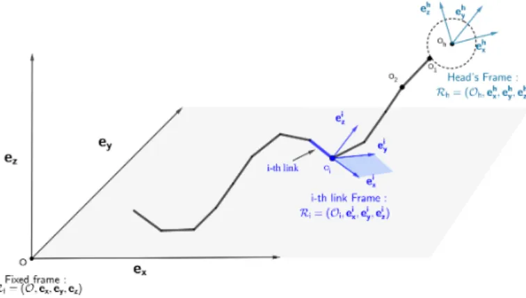
Fig. 1. Reference and local frames of the discrete-shape model. The swimmer’s head frame is oriented relative to the reference frame. For each link i, the
correspond-ing local frame Ri is oriented relative to Rh.
We associate to the head of the swimmer the moving
frame Rhead = (Oh, ehx, e
h y, e
h
z), where Oh is the center
of the head. The orientation of each link i is represented
by the moving frame Ri = (Oi, eix, e
i y, e
i
z), where Oi is
the extremity of the i-th link. We define Rhead ∈ SO(3)
as the rotation matrix that allows the transformation of
coordinates from the fixed reference frame to Rhead and
the matrices Ri ∈ SO(3), for i = 1 · · · N , as the relative
rotation matrix that transforms coordinates from Rhead
to Ri. Rhead is parametrized by a (X − Y − Z) rotation
sequence (θx, θy, θz) and each relative rotation matrix Ri
is parametrized by a Y − Z rotation sequence : (φiy, φiz)
relative to the head’s frame. Using these notations, the swimmer is represented by two sets of variables : The Position variables: (X, Θ) where
X = (xh, yh, zh) ∈ R3 and
Θ = (θx, θy, θz) ∈ [0, 2π]3,
(1)
and the 2N Shape variables, denoted by
Φ = (φ1y, φ1z, · · · , φNy , φNz) ∈ [0, 2π]2N. (2) 2.2 Dynamics of the swimmer
The RFT framework neglects the global interactions be-tween the swimmer and the surrounding fluid in favor of the local anisotropic friction of the slender body with the surrounding fluid. This results in explicit expressions of the density of force applied by the fluid to the swimmer
that are linear with respect to ( ˙X, ˙Θ, ˙Φ). More precisely,
We consider a hydrodynamical drag force Fhhead acting
on the head of the swimmer that is proportional to its velocity in each of the direction of the head’s frame’s
vectors Rhead and a hydrodynamical torque on the head
that is proportional to its angular velocity :
Fhhead= −RheadDHRTheadX˙
Thhead= −kRΩhead.
(3)
where kH,k, k1H,⊥, and kH,⊥2 are positive real numbers that
represents the hydrodynamic drag coefficients of the head
along the eh
x, e h
y and e
h
z direction, DH is the matrix
kH,k 0 0 0 k1H,⊥ 0 0 0 kH,⊥2
,kR is the rotational drag coefficient
of the head and Ωheadis the angular velocity vector of the
head of the swimmer.
To compute the hydrodynamic effects on each link i ∈ (1, · · · , N ) of the tail, we consider the hydrodynamic force
density fi(s) acting on a point xi(s) parametrized by
its arclength s. Following Resistive Force Theory, the
expression of fi(s) reads : fi(s) = −kk(Vi(s).eix)e i x− k⊥(Vi(s).eiy)e i y − k⊥(Vi(s).eiz)e i z (4)
where kk and k⊥are respectively the parallel and
perpen-dicular drag coefficients of the swimmer and Vi(s) is the
velocity of xi(s).
The drag force on link i, Fhi, and hydrodynamic torques
on each link i (about the extremity Oj of link j derive
from the force densities as follows:
Fhi = Z l 0 fi(s)ds , (5) and ∀j ∈ (1 · · · N ) Th i,Oj = Z l 0 (xi(s) − Oj) × fi(s)ds , (6)
where l is the length of each link.
We consider that the head of the swimmer is magnetized
along the eh
x axis. Denoting by M the magnetization
vec-tor of the head and considering an external homogeneous time-varying field B(t), the following torque is applied to the swimmer
Tmag = M × B(t). (7)
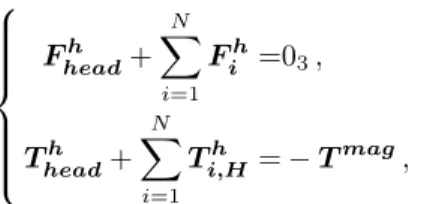
The acceleration terms in the dynamics are neglected due to the Low Reynolds assumption (Yates (1986)), thus, the balance of forces and torques applied on the swimmer gives:
Fheadh + N X i=1 Fih=03, Theadh + N X i=1 Ti,Hh = − Tmag, (8)
which leads to 6 independent equations. In addition to these equations, we take the internal contributions of the tail and its elasticity into account by adding the balance of torque on each subsystem consisting of the chain formed by the links i to N for i = 1 · · · N . These 3N equations reduce to 2N non-trivial equations by taking only the components perpendicular to the link k when calculating the sum of the torques from k to N . The elasticity of the tail is discretized
by considering a restoring elastic moment Tielat each joint
Oithat tends to align each pair (i, i + 1) of adjacent links
with each other:
Tiel= keleix× ei−1x . (9)
Thus, the dynamics of the swimmer are described the following system of 2N + 6 equations :
Fheadh + N X i=1 Fih= O3, Theadh + N X i=1 Ti,Hh = −Tmag, N X i=1 Ti,1h .e1y= −T1el.e1y, N X i=1 Ti,1h .e1z= −T1el.e1z, .. . .. . TN,Nh .eny = −Tnel.eny, TN,Nh .enz = −Tnel.enz. (10)
Following Resistive Force Theory, and the definition of the drag densities, the hydrodynamic contributions (left-hand side of the previous system) are linear with respect to the angular and translational velocities, thus, the previous equation can be rewritten matricially in the form :
Mh(Θ, Φ) ˙ X ˙ Θ ˙ Φ = B(X, Θ, Φ). (11)
, where Mh(Θ, Φ) ∈ R(2N +6)×(2N +6represents the
hydro-dynamical effects on the swimmer and the right-hand side
B(X, Θ, Φ) ∈ R2N +6 corresponds to the magnetic and
elastic contributions on the swimmer.
The previous equation can be rewritten as a control system, where the dynamics of the swimmer are affine with respect to the components of the actuating magnetic field viewed as a control: ˙ X ˙ Θ ˙ Φ = F0(Θ, Φ) + (Bx(t) By(t) Bz(t)) F1(Θ, Φ) F2(Θ, Φ) F3(Θ, Φ) ! (12)
where the vector fields F0, · · · , F3 are functions of the
columns of (Mh)−1 and of the magnetic and elastic
con-stants.
3. SWIMMING WITH SINUSOIDAL FIELDS The most commonly used actuating strategy for straight swimming in experiments is to apply the superposition of a static magnetic field to orient the swimmer in the desired direction and a perpendicular sinusoidal field to actuate the swimmer. This induces a planar symmetric beating of the tail of the swimmer, allowing a horizontal displacement. This actuation strategy will be used as a benchmark to compare with the optimal solutions. The hydrodynamical and elastic parameters of the model were fitted on experimental data (El Alaoui-Faris et al. (2020)) .for the characterization of the swimmer. Using these parameters, we are able to simulate the velocity-frequency response curve of the swimmer (Fig. 3), using a magnetic field of the form :
B(t) = (Bx, Bysin(2πf t), 0) . (13)
The velocity-frequency response curve of the swimmer shows a behaviour typical of flagellar low Reynolds swim-mers, as it shows an increase of the swimming velocity until a cut-off frequency (1.5 Hz) where the velocity decreases slowly beyond this value.
Frequency (Hz) 0 0.5 1 1.5 2 2.5 3 3.5 4 M ean p rop u ls ion sp ee d ( m m. s − 1) 0 0.2 0.4 0.6 0.8 1 1.2
Fig. 2. Simulated velocity-frequency response curve of the swimmer.
4. OPTIMAL CONTROL PROBLEMS
The purpose of this paper is to find the time-varying mag-netic field B =
Bx(t)
By(t)
Bz(t)
!
that maximizes the horizontal
displacement of the swimmer at a fixed time tf. Denoting
by Z(t) the state vector X(t) Θ(t) Φ(t)
!
and rewriting equation
(12) as ˙Z(t) = f (Z(t), B(t)), this optimal control
max x(tf) ˙ Z(t) = f (Z(t), B(t)) Z(0) = 0 B(t) ∈ C , (14)
where C is the set of constraints on the magnetic field and tf is the final time fixed at 3s . We investigate four optimal control problems depending on the types of constraints on the actuating magnetic field, taking in each case the same bounds on the magnetic field intensities.
(1) In the first optimal control problem (OCP1), we consider the admissible controls as the superposition of a static orientating field along the x axis and a time-varying field along the y axis :
C1= {B(t), Bx(t) = 2.5mT, |By| ≤ 10mT, Bz(t) = 0}
(2) In the second optimal control problem (OCP2), both the x and y components of the magnetic field are time-varying.
C2= {B(t), Bz(t) = 0, ||(Bx(t), By(t))|| ≤ 10mT }
(3) In the third problem (OCP3), we consider the ad-missible controls to be the superposition of a static orientating field along the x axis and a time-varying actuating field in the y − z plane.
C3= {B(t), Bx= 10mT ||(Bz(t), By(t))|| ≤ 10mT }
(4) In the last optimal control problem (OCP4), we consider the general case where all components of the magnetic field are time-varying.
C4= {B(t), ||(Bx(t), Bz(t), By(t))|| ≤ 10mT }
5. NUMERICAL SOLUTIONS
We use a direct method for solving the aforementioned optimal control problems. The optimal control solver ICLOCS (Falugi et al. (2010)) is used for the resolution. It discretizes the problem into a non-linear programming problem which is then solved by the interior-point solver
IPOPT (W¨achter and Biegler (2006)). Fig. 3 shows the
displacements of the swimmer under each optimal solution, and under the sinusoidal field at the optimal frequency (1.5 Hz). We see that non-planar solutions largely out-performs planar solutions. None of the optimal solutions display singular arcs. Accordingly, and following Pontrya-gin’s maximum principle, the solution of the single input problem OCP1 is a sequence of bang arcs and the solutions of the other problems are continuous.
0 0.5 1 1.5 2 2.5 3 3.5 t (s) -2 0 2 4 6 8 10 12 Solution - OCP4 Solution - OCP3 Solution - OCP2 Solution - OCP1 Sinusoidal Field
Fig. 3. Comparison of x-displacements associated with the solutions of OCP1-4 and with the sinusoidal actuation
5.1 Planar Solutions
For OCP1 and OCP2, the dimension of the dynamic system reduces to N+3 because of the fact that the con-straints on the controls leads to a planar trajectory in the x − y plane. The numerical solution for OCP1 takes the form of a sequence of Bang arcs, as seen in Fig. (4, (a) ) whereas the solution of OCP2 is continuous ((b), (c)). In both cases, the optimal actuation patterns lead to a trajectory where swimmer oscillates around the x axis while moving in the x-direction (see Fig. 5).
The shape of both optimal trajectories is similar to the trajectory of the swimmer under the sinusoidal field. Inter-estingly enough, the optimal magnetic fields are periodic in both cases, and induce a periodic deformation of the swimmer, as seen in Fig. 6. Both solutions out-perform the reference sinusoidal actuation in terms of horizontal speed.
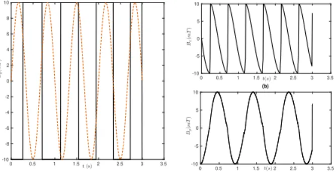
In practice, the solution of OCP-1 shows that having an orthogonal actuating field (in addition to the static orientating field) in the form of a square signal is more efficient than an actuating sinusoidal field. The solution of the second planar problem (OCP-2) shows that ori-entating fields are not necessary for straight swimming and that actuating a flagellar magnetic swimmer with two time-varying components leads to a substantial increase in swimming speed. 0 0.5 1 1.5 2 2.5 3 3.5 -10 -8 -6 -4 -2 0 2 4 6 8 10 (a) 0 0.5 1 1.5 2 2.5 3 3.5 -10 -5 0 5 10 (b) 0 0.5 1 1.5 2 2.5 3 3.5 -10 -5 0 5 10 (c)
Fig. 4. Solution of the planar optimal control problems. (a) : y-component of the solution of OCP-1 compared with the sinusoidal field at optimal frequency (1.5Hz). (b): x-component of the solution of OCP-2. (c) : y-component of the solution of OCP-3.
-1 0 1 2 3 4 5 6 7 x (mm) -1.2 -1 -0.8 -0.6 -0.4 -0.2 0 0.2 0.4 0.6 0.8 y (mm) OCP-1 OCP-2 Sinusoidal Field
Fig. 5. Optimal planar trajectories associated with OCP-1 and OCP-2 compared with the trajectory of the swimmer actuated by the sinusoidal field.
Fig. 6. Shape angles of the swimmer for the solutions of both planar problems OCP-1 and OCP-2.
5.2 Non-planar solutions
The non-planar optimal magnetic fields solutions of OCP3 and OCP4 leads to trajectories ,shown in Fig. 8, where the swimmer revolves around the horizontal axis.
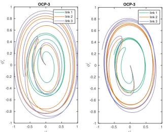
As seen in Fig. 3, the non-planar actuation patterns largely out-performs the planar ones, which shows the necessity of allowing flagellar swimmers to go out-of-plane in order to swim at a maximal propulsion speed. Similarly to the planar case, the optimal solution is periodic apart from transient states near the initial and final times (see Fig. 7) and induce a periodic 3D deformation of the tail of the swimmers, as shown in the phase planes of Fig. 9.
0 0.5 1 1.5 2 2.5 3 -10 -5 0 5 10 (b) 0 0.5 1 1.5 2 2.5 3 -10 -5 0 5 10 (a) 0 0.5 1 1.5 2 2.5 3 -5 0 5 (c) 0 0.5 1 1.5 2 2.5 3 -10 -5 0 5 10 (e) 0 0.5 1 1.5 2 2.5 3 -10 -5 0 5 10 (d)
Fig. 7. Solution of the non-planar optimal control prob-lems. (a) : y-component of the solution of OCP-3. (b): z-component of the solution of OCP-2. (c) : x-component of the solution of OCP-4. (d) : y-component of the solution of OCP-4. (e) : z-component of the solution of OCP-4.
-1.2 -1 0.8 -0.8 -0.6 -0.4 0.6 -0.2 0 0.4 0.2 0.4 0.2 0.6 0 -0.2 12 10 -0.4 8 6 4 -0.6 2 0 OCP-4 OCP-3
Fig. 8. Trajectories of the swimmer associated with the solutions of OCP-3 and OCP-4.
-1 -0.5 0 0.5 1 -1 -0.8 -0.6 -0.4 -0.2 0 0.2 0.4 0.6 0.8 1 OCP-3 link 1 link 2 link 3 -1 -0.5 0 0.5 1 -1 -0.8 -0.6 -0.4 -0.2 0 0.2 0.4 0.6 0.8 1 OCP-3 link 1 link 2 link 3
Fig. 9. Shape variables of the swimmer when actuated by the non-planar optimal magnetic fields (OCP3 and OCP4). Phase portrait of the relative angles in the (φiy− φi
z) for each link i of the tail.
5.3 Influence of the number of links on the trajectory and shape of the swimmer
An analysis of the influence of the number of links of the model on the optimal trajectories and magnetic fields have been made for OCP4. We define the relative trajectory
error Etr as :
Etr =
||XN− XN −1||∞
||XN||∞
, (15)
where XN is the optimal trajectory using N links for the
tail. Similarly, we define the relative solution error Esol as
:
Esol=
||BN− BN −1||∞
||BN||∞
, (16)
where BN is the optimal magnetic field using N links for
the tail.
Fig. 10 shows the evolution of the relative trajectory and solution errors for N = (1 · · · 9). We notice that the optimal magnetic field and the optimal trajectory only marginally changes when increasing the number of links beyond 3. This shows that a 3-linked tail is enough for the optimization of the actuation of flagellar magnetic swim-mers, which further emphasizes the low computational cost of our model.
Fig. 10. Relative optimal trajectories and solution errors for an increasing number of links of the tail of the swimmer.
6. CONCLUSION AND PERSPECTIVES In this paper, we have presented a simplified 3D dynamical model for flagellar micro-swimmers based on Resistive Force Theory and shape discretization, which circumvents the numerical drawbacks of continuum mechanics-based models. This model was used to investigate different planar and non-planar optimal actuation strategies for magnetic micro-swimmers that out-perform the commonly used si-nusoidal actuation. In particular, the non-planar actuation strategies lead to a novel 3D trajectory and are signifi-cantly more efficient than the planar ones.
Another result stemming from the numerical simulations is the investigation of optimal actuation strategies that do not rely on a static orientating magnetic field, as allowing all the components of the magnetic field to be time-varying leads to an increase in swimming speed. However, these actuation methods lead to larger oscillations of the swim-mer around the swimming direction, which could be an inconvenient for some experimental settings such as path following.
Beyond the present study, the simplified model presented in our model allows for easy numerical optimization studies for micro-swimmers such as parameter fitting or optimal motion planning for magnetic swimmers. It has been suc-cessfully used to optimize the displacements of an ex-perimental swimmer in (El Alaoui-Faris et al. (2020)). It can also be easily adapted to model biological flagel-lar micro-swimmers. Ongoing work includes optimization of the swimming speed for more complex cost functions (maximization of efficiency, path following ..) and adapting the model for swimming in complex environments (for example in a narrow channel or in presence of a wall). Theoretical study of the optimal control problems is also a perspective of this work.
REFERENCES
Alouges, F., DeSimone, A., Giraldi, L., and Zoppello, M. (2013). Self-propulsion of slender micro-swimmers by curvature control: N-link swimmers. International Journal of Non-Linear Mechanics, 56, 132–141.
Alouges, F., DeSimone, A., Giraldi, L., and Zoppello, M. (2015). Can magnetic multilayers propel artificial microswimmers mimicking sperm cells? Soft Robotics, 2(3), 117–128.
Dreyfus, R., Baudry, J., Roper, M.L., Fermigier, M., Stone,
H.A., and Bibette, J. (2005). Microscopic artificial
swimmers. Nature, 437(7060), 862.
El Alaoui-Faris, Y., Pomet, J.B., R´egnier, S., and Giraldi,
L. (2020). Optimal actuation of flagellar magnetic
microswimmers. Physical Review E, 101(4), 042604. Falugi, P., Kerrigan, E., and Wyk, E. (2010). Imperial
college london optimal control software (iclocs). Online: http://www. ee. ic. ac. uk/ICLOCS.
Fusco, S., Sakar, M.S., Kennedy, S., Peters, C., Bottani,
R., Starsich, F., Mao, A., Sotiriou, G.A., Pan´e, S.,
Pratsinis, S.E., et al. (2014). An integrated microrobotic platform for on-demand, targeted therapeutic interven-tions. Advanced Materials, 26(6), 952–957.
Gray, J. and Hancock, G. (1955). The propulsion of sea-urchin spermatozoa. Journal of Experimental Biology, 32(4), 802–814.
Khalil, I.S., Dijkslag, H.C., Abelmann, L., and Misra, S.
(2014). Magnetosperm: A microrobot that navigates
using weak magnetic fields. Applied Physics Letters,
104(22), 223701.
Lowe, C.P. (2003). Dynamics of filaments: modelling the dynamics of driven microfilaments. Philosophical Trans-actions of the Royal Society of London B: Biological Sciences, 358(1437), 1543–1550.
Mack, M.J. (2001). Minimally invasive and robotic
surgery. Jama, 285(5), 568–572.
Moreau, C., Giraldi, L., and Gadelha, H.A.B. (2018). The asymptotic coarse-graining formulation of slender-rods, bio-filaments and flagella. Journal of the Royal Society Interface.
Oulmas, A., Andreff, N., and R´egnier, S. (2017). 3d
closed-loop motion control of swimmer with flexible flagella at low reynolds numbers. In Intelligent Robots and Systems (IROS), 2017 IEEE/RSJ International Conference on, 1877–1882. IEEE.
Patra, D., Sengupta, S., Duan, W., Zhang, H., Pavlick, R., and Sen, A. (2013). Intelligent, self-powered, drug delivery systems. Nanoscale, 5(4), 1273–1283.
Qiu, F., Fujita, S., Mhanna, R., Zhang, L., Simona, B.R., and Nelson, B.J. (2015). Magnetic helical microswim-mers functionalized with lipoplexes for targeted gene delivery. Advanced Functional Materials, 25(11), 1666– 1671.
Tornberg, A.K. and Shelley, M.J. (2004). Simulating the dynamics and interactions of flexible fibers in stokes flows. Journal of Computational Physics, 196(1), 8–40.
W¨achter, A. and Biegler, L.T. (2006). On the
implemen-tation of an interior-point filter line-search algorithm
for large-scale nonlinear programming. Mathematical
programming, 106(1), 25–57.
Yates, G.T. (1986). How microorganisms move through water: the hydrodynamics of ciliary and flagellar propul-sion reveal how microorganisms overcome the extreme effect of the viscosity of water. American scientist, 74(4), 358–365.
Ye, Z., R´egnier, S., and Sitti, M. (2014). Rotating
mag-netic miniature swimming robots with multiple flexible flagella. IEEE Transactions on Robotics, 30(1), 3–13.