HAL Id: hal-02370259
https://hal.archives-ouvertes.fr/hal-02370259
Submitted on 22 Nov 2019HAL is a multi-disciplinary open access archive for the deposit and dissemination of sci-entific research documents, whether they are pub-lished or not. The documents may come from teaching and research institutions in France or abroad, or from public or private research centers.
L’archive ouverte pluridisciplinaire HAL, est destinée au dépôt et à la diffusion de documents scientifiques de niveau recherche, publiés ou non, émanant des établissements d’enseignement et de recherche français ou étrangers, des laboratoires publics ou privés.
Population persistence under high mutation rate: from
evolutionary 1 rescue to lethal mutagenesis
Yoann Anciaux, Amaury Lambert, Ophélie Ronce, Lionel Roques, Guillaume
Martin
To cite this version:
Yoann Anciaux, Amaury Lambert, Ophélie Ronce, Lionel Roques, Guillaume Martin. Population persistence under high mutation rate: from evolutionary 1 rescue to lethal mutagenesis. Evolution -International Journal of Organic Evolution, Wiley, 2019, 73 (8), pp.1517-1532. �10.1111/evo.13771�. �hal-02370259�
Population persistence under high mutation rate: from evolutionary
1rescue to lethal mutagenesis
2Yoann Anciaux1, 2 Amaury Lambert3, 4 Ophélie Ronce1 Lionel Roques5 Guillaume Martin1 3 4 1 ISEM ‐ Institut des Sciences de l'Evolution de Montpellier, France 5 2 BiRC ‐ Bioinformatics Research Center, Aarhus Danemark 6 3 CIRB ‐ Centre interdisciplinaire de recherche en biologie, Paris, France 7 4 LPSM UMR 8001 ‐ Laboratoire de Probabilités, Statistique et Modélisation, Paris, France 8 5 INRA ‐ Biostatistics and Spatial Processes (BioSP), Avignon, France 9 10
Contacts : [email protected] , [email protected]
11 12 Keywords : Evolutionary rescue, Fisher’s Geometric Model, Fitness landscape, Lethal mutagenesis, 13 Extinction dynamics, Distribution of extinction times 14
15
Abstract
16
Populations may genetically adapt to severe stress that would otherwise cause their 17 extirpation. Recent theoretical work, combining stochastic demography with Fisher’s geometric 18 model of adaptation, has shown how evolutionary rescue becomes unlikely beyond some critical 19 intensity of stress. Increasing mutation rates may however allow adaptation to more intense stress, 20
raising concerns about the effectiveness of treatments against pathogens. This previous work 21
assumes that populations are rescued by the rise of a single resistance mutation. However, even 22
in asexual organisms, rescue can also stem from the accumulation of multiple mutations in a single 23
genome. Here, we extend previous work to study the rescue process in an asexual population 24
where the mutation rate is sufficiently high so that such events may be common. We predict both 25
the ultimate extinction probability of the population and the distribution of extinction times. We 26
compare the accuracy of different approximations covering a large range of mutation rates. 27 Moderate increase in mutation rates favors evolutionary rescue. However, larger increase leads to 28 extinction by the accumulation of a large mutation load, a process called lethal mutagenesis. We 29 discuss how these results could help design “evolution‐proof” anti‐pathogen treatments that even 30 highly mutable strains could not overcome. 31
32
Introduction
33 Evolutionary rescue (ER) happens when a population confronted with severe stress avoids 34 extinction by genetic adaptation. Understanding and predicting when and how evolutionary rescue 35 occurs is critical in fields as diverse as conservation biology, invasion biology, emergence of new 36 diseases and the management of resistance to treatment in pests and pathogens (see reviews in 37 Gonzalez et al. 2013; Carlson et al. 2014; Alexander et al. 2014; Bell 2017). In all these situations, 38genetic variation, be it present before the onset of stress, or generated de novo after, is a key 39 ingredient for evolutionary rescue, as expected theoretically (e.g. Gomulkiewicz and Holt 1995) 40 and observed experimentally (e.g Ramsayer et al. 2013). Because mutation affects both standing 41 and de novo genetic variation, it comes as no surprise that a number of evolutionary rescue models, 42
combining stochastic evolution and demography, have predicted that higher mutation rates are 43
associated with higher probability of evolutionary rescue (Orr and Unckless 2008, 2014; Martin et 44
al. 2013; Anciaux et al. 2018). Few evolutionary rescue experiments have manipulated the 45
mutation rate to test these predictions (reviewed in Bell 2017). For instance, Couce et al. (2015) 46
found that two different mutator strains of bacteria with elevated rates of mutations evolved more 47
than 100‐fold resistance to antibiotic concentrations that caused the demise of control strains. 48 Mutator alleles are indeed often found in antibiotic resistant strains causing serious health issues 49 (Eliopoulos and Blázquez 2003), raising concern about pathogens escaping our control by evolving 50 higher mutation rates (for theoretical predictions see Taddei et al. 1997; Greenspoon and Mideo 51 2017). 52 Most mathematical models of evolutionary rescue assume that the population is rescued 53
from extinction by the spread of a single mutant of large effect (Orr and Unckless 2008, 2014; 54
Martin et al. 2013; Anciaux et al. 2018) and do not describe highly polymorphic populations where 55
several mutations of smaller effects can combine to allow population growth (see however the 56
work of Uecker and Hermisson (2016) and Uecker (2017) where sexual reproduction allows 57
production of such rescue genotypes). The latter situation seems in particular to be common in 58
the evolution of herbicide resistance, especially when the mutational target for resistance is large 59
(Kreiner et al. 2018). Even in asexual organisms, when the mutation rate is high, evolutionary 60
rescue may commonly result from the cumulative effect of multiple mutations accumulating 61 stochastically over time in a given lineage. Such a mutation regime is particularly relevant in highly 62 mutable viruses, mutator strains of bacterial (e.g. Springman et al. 2010) or cancer cells (e.g. Loeb 63 2001). Our aim here is to provide theoretical predictions for evolutionary rescue in such a regime 64 with high mutation rates in asexual organisms, complementing existing theory on the subject. 65
Several complications arise when modelling evolutionary rescue in highly polymorphic 66
populations with high mutation rates. First, the dynamics of allelic frequencies at different loci 67 interact in asexuals. For example, the selective sweep of a given beneficial mutation is hindered by 68 the co‐segregation of other beneficial mutations (clonal interference, Gerrish and Lenski 1998). A 69 theoretical study by Wilson et al. (2017) recently showed that, when evolutionary rescue is likely, 70
it should most often be driven by soft selective sweeps, where multiple resistance mutations 71
spread through the population simultaneously. Wilson et al. (2017) still assumed that each of these 72 lineages carried a single mutation, each with the same effect on the population growth rate. When 73 the mutational target is large, different lineages contributing to rescue are however likely to carry 74 mutations with different fitness effects. Modelling the distribution of mutation effects (as in Martin 75 et al. 2013; Anciaux et al. 2018) then becomes critical. Finally, when the mutation rate is high, 76 multiple mutations may also accumulate in each lineage, either facilitating evolutionary rescue or 77 impeding it, through their cumulative effect. Modelling both beneficial and deleterious mutations 78 and, critically, the epistatic interactions between them, also becomes necessary. 79 Previous evolutionary rescue theory predicts that higher mutation rate allows populations 80 to withstand higher levels of stress (e.g. Anciaux et al. 2018). Yet, there are reasons to expect this 81 prediction not to hold above some critical mutation rate: increased mutation rates also build‐up 82
detrimental mutation loads, thus depressing mean fitness despite ongoing adaptation. Indeed, 83
some previous ER models, including both beneficial and deleterious additive effects on growth 84
rates, have found that ER was most likely at intermediate mutation rates (Loverdo and Lloyd‐Smith 85
2013; Greenspoon and Mideo 2017). Artificially increasing the mutation rate has even been 86
proposed as a means to weaken or even eliminate pathogen populations, by a process called lethal 87
mutagenesis (Loeb et al. 1999). Models of lethal mutagenesis predict that extinction of the target 88
population could be observed under biologically realistic sets of parameters (Bull et al. 2007; 89
Martin and Gandon 2010; Wylie and Shakhnovich 2012). In these models, mean fitness dynamics 90
and extinction stem from the deterministic effects of selection and mutation. Alternatively, 91 Matuszewski et al. (2017) discuss the continuity between these models and models of mutational 92 meltdown, where extinction is driven by the interaction of genetic drift and deleterious mutation. 93 Lethal mutagenesis has been investigated empirically for treatment against viruses (Springman et 94
al. 2010; Arias et al. 2014), bacteria (Bull and Wilke 2008) or cancer cells (Liu et al. 2015). In 95
particular, the combination of antiviral treatments with mutagenic agents is investigated as a 96 strategy to fight fast evolving viruses, such as influenza (Bank et al. 2016). It seems important to 97 improve our ability to predict whether and when such mutagenic agents will increase treatment 98 efficacy or, conversely, facilitate the evolution of resistance. 99
The population genetics of adaptation behind the rescue process, in isolated asexual 100 populations, roughly fall into two alternative regimes: rescue may stem (i) from single mutations 101 of large effect (strong selection weak mutation ‘SSWM’ regime) or (ii) from multiple mutations of 102 small effects (weak selection strong mutation ‘WSSM’ regime) (reviewed in Alexander et al. 2014). 103
The dichotomy between SSWM and WSSM entails a somewhat simplistic view of adaptation 104
regimes, at the two extremes of all possible mutation rates. The SSWM regime of adaptation has 105
been extensively investigated in population genetics via “origin‐fixation” models describing the 106
average behavior of stochastic evolutionary dynamics (McCandlish and Stoltzfus 2014) whereas 107
the WSSM regime has been widely analyzed via deterministic models of quantitative genetics 108
(Lande 1976, 1980). Corresponding evolutionary rescue models further include a coupling of 109 adaptation and demographic dynamics, and naturally fall into the same two regimes (discussed in 110 Anciaux et al. 2018). The SSWM regime of evolutionary rescue is characterized by the fact that the 111 first resistant lineage to establish (and thus cause rescue) is only one mutational step from the 112
predominant, sensitive ‘wild‐type’ lineage (e.g. Feder et al. 2016). Models that describe highly 113
polymorphic dynamics (WSSM regimes, e.g. the quantitative genetic model in Gomulkiewicz and 114
Holt 1995) often use the infinitesimal model assumptions (many unlinked polymorphic loci), which 115
does not apply to asexual populations. In the WSSM regime, the exact stochastic evolutionary 116
dynamics become quickly intractable, and have often been studied by simulation (e.g. Boulding 117
and Hay 2001). Further the latter models often consider initial standing genetic variance as given 118
and pay little attention to the effect of mutation rates in maintaining this variance. They often 119 ignore de novo mutations after the onset of stress, on the argument of short timescales being most 120 critical for evolutionary rescue (e.g. Gomulkiewicz et al. 2010). 121 To make analytical progress in our understanding of the effect of mutation rates on the 122
process of evolutionary rescue, we build on two recent theoretical developments (Martin and 123
Roques 2016; Anciaux et al. 2018). Anciaux et al. (2018) developed a model of evolutionary rescue 124
in the SSWM regime using Fisher’s (1930) geometric model (hereafter "FGM") to model the 125
distribution of mutation effects on fitness. As in Anciaux et al. (2018), we study evolutionary rescue 126
using the FGM. This model assumes a single peak phenotype‐fitness landscape, where fitness 127
depends on the position, in phenotype space, of a given genotype relative to an optimum. In the 128
context of ER, stress may affect this landscape in various ways (height, width or position of the 129 peak). In this model, the distribution of mutation effects (both beneficial and deleterious) depend 130 on the context, both genotypic (epistasis) and environmental (e.g. effect of stress). This context‐ 131 dependence is a key feature of the FGM; it is absent from previous ER models studying the effect 132 of high mutation rates, because they assume additive mutation effects on fitness (e.g. Loverdo and 133
Lloyd‐Smith 2013; Greenspoon and Mideo 2017). The variation in the distribution of mutation 134 effects implied by the FGM is qualitatively, and sometimes even quantitatively, consistent with a 135 wealth of empirical observations (reviewed in Tenaillon 2014). Under the assumptions of the FGM, 136 rescue mutants become very rare as the intensity of stress increases, because they require very 137
large mutational steps. As a consequence, Anciaux et al. (2018) predict that there is a narrow 138 window of stress levels where the probability of rescue shifts from being very likely to very unlikely. 139 They also predict that this critical level of stress, beyond which adaptation is unlikely, is increased 140 by higher mutation rates (Anciaux et al. 2018). Yet, predictions of this model apply to the SSWM 141 regime and may not hold for higher mutation rates. 142
We extend our previous analysis of evolutionary rescue over Fisher’s geometric model 143
(Anciaux et al. 2018) to the more complex and more polymorphic WSSM regime. To do so, we use 144
the approach in Martin and Roques (2016) to model the non‐equilibrium dynamics of fitness 145
distributions, in large asexual populations. The form of fitness epistasis assumed may have 146 particular impact on the results because lineages accumulate multiple mutations at different sites 147 over the rescue process. We use the FGM here, which implies a particular form of epistasis that 148 has proven consistent with several observed patterns in fitness epistasis among mutations (Martin 149
et al. 2007; Perfeito et al. 2014; Blanquart and Bataillon 2016). Moreover, Martin and Roques 150
(2016) showed that, under the FGM, while the fitness dynamics are more complex at higher 151
mutation rates, they are also more predictable and less prone to stochastic fluctuations, even in 152
relatively small populations. To model evolutionary rescue, we still need to describe the 153
demographic stochasticity associated with the extinction process. In the WSSM regime, we thus 154
use a combination of two analytically tractable theories: a deterministic approximation to the 155
dynamics of mean fitness (Martin and Roques 2016) and a diffusion approximation to the 156
stochastic dynamics of population sizes (from Bansaye and Simatos 2015). 157
Beyond a derivation of the probability of ultimate rescue or extinction, this approach 158
further allows tracking the rescue process over time. As stated in Gomulkiewicz et al. (2017), 159
tracking of transient dynamics (population size dynamics, distributions of extinction times) are of 160
high interest for applications of evolutionary rescue theory, yet are not available from existing 161
predictions, which focused mainly on ultimate outcomes. Gomulkiewicz et al. (2017) studied the 162
distribution of extinction times for populations doomed to extinction, mostly in the absence of 163
mutation (i.e. with a fixed arbitrary set of competing asexual genotypes at the onset of stress). We 164
extend this analysis to include frequent de novo mutation, rescue events involving several 165
mutational steps, a particular form of epistasis and variable mutation effects depending on stress 166
intensity, and an explicit description of the dynamics of mutation load. Our approach captures the 167
continuum from evolutionary rescue to lethal mutagenesis, as mutation rate increases. 168
Interestingly, some parameter ranges prove to greatly limit evolutionary rescue at all mutation 169 rates, i.e. in spite of the possible mutator genotypes. 170 171
Methods
172 I. General framework 173The present work focuses on an asexual population with independent lineages (e.g. a 174
population of asexual microbes without horizontal gene transfer), facing an abrupt and stressful 175
environmental change (e.g. an antimicrobial treatment). The population initially consists of 176
individuals with either a single or multiple genotypes and is initially adapted to a non‐stressful 177
environment, where its mean growth rate is positive. At the onset of stress, the population is 178 shifted from the non‐stressful environment to a stressful environment, where its mean growth rate 179 becomes negative (definition of stress here). In such an environment, in the absence of evolution, 180 the population is doomed to extinction. Evolutionary rescue occurs if at least one resistant lineage 181
(with a positive growth rate in the new environment) establishes, in spite of demographic 182 stochasticity. These resistant mutant lineages can either already be present in the population or 183 arise de novo after the onset of stress. It is thus crucial to determine how the number and growth 184 rates of such mutants depend on the new environmental conditions and on the parental genotypes 185
already present in the population. We do so using the FGM detailed below. Note that the main 186 notations used here are summarized in Table 1. 187 188 Fitness landscape 189
In the FGM, a given phenotype is a vector in a phenotypic space of dimensions that 190
determine fitness (here the growth rate ). The phenotype of an individual with genotype , is 191
characterized by a vector ∈ of the breeding values (heritable components) for the traits, 192
and its growth rate is . In a given environment, fitness decays as a quadratic function of the 193
phenotypic distance to a single phenotypic optimum, where the growth rate is maximal at a 194
given absolute level (height of the fitness peak). We assume that each environment is associated 195
with a single optimum and fitness peak. In the scenario investigated here, in the non‐stressful 196
environment, the population is close to the ‘ancestral’ optimum . When the environment 197
changes, it is assumed to determine a new optimum ∗. Without loss of generality, the height of
198
the peak may also differ between the ancestral and new environments. However, we do require 199
that the dimensions that determine fitness remain the same (in nature and number) across 200 environments. In the new environment, the growth rate of an individual with genotype is given 201 by: 202 , ⋆ ‖ ∗‖ 2 . [1] This is an isotropic version of the FGM (all directions are equivalent for selection and mutation) 203 where phenotypes are scaled by selective strength. 204 205 Stochastic demographic dynamics 206 We confine our analysis to finite haploid asexual populations. Individuals have independent 207 evolutionary and demographic fate (frequency or density dependence are ignored). Each genotype 208
has a growth rate and a reproductive variance ( , ∗ in a given environment with
optimum ∗), which define its stochastic demographic parameters in the context of a Feller 210 diffusion approximation (Feller 1951), as in e.g. Martin et al. (2013), Gomulkiewicz et al. (2017) or 211 Anciaux et al. (2018). For simplicity, we further assume here that the average stochastic variance 212 in reproduction is constant over time∶ 1⁄ ∑ , where the average is taken over 213
the genotypes present at time . This can for example be accurate whenever the are roughly 214
constant across genotypes (discussed in Martin et al. 2013 and Anciaux et al. 2018). 215
216
Notation Description Formula
, : population size at time after the onset of the stress.: initial population size at the onset of the stress.
Mutation rate per individual per unit time.
Number of traits under stabilizing selection, or phenotypic dimensionality. Variance of mutational effects: variance of the phenotypic effects of mutations, per trait, in a trait
space scaled by the strength of stabilizing selection ~ , Composite parameter : square root of mutational variance per trait √
phenotype ‐dimensional vector ∈ of (breeding values for) , ∗ ∗: optimal phenotype in the new environment : average phenotype of the ancestral population
(before the onset of stress)
, Growth rate ( ) and reproductive variance ( ) of a given genotype, in the new environment. Eq.[1] , Mean growth rate (( ) of the population, in the new environment. and mean reproductive variance Eqs. [2] and [3] 〈 〉 ‘ensemble mean’ growth rate : expected mean growth rate ̅ across stochastic replicates Eqs. [2] and [3]
Maximum possible growth rate in the new environment. ∗
Rate of decay of the ancestral phenotypeenvironment. in the new ‖ ‖ 2⁄
Rate of decay scaled by . ⁄ Ratio between the mutational load and the maximal growth rate / 2 , : rate of rescue from de novo mutations scaled by : rate of rescue from both de novo and standing variance scaled by Eqs.[5],[6]
Critical mutation rate beyond which the WSSM regime is valid. /4 Mutation rate beyond which certain extinction is enforced by lethal mutagenesis 4 /
∗ Mutation rate at which the rescue probability rises to 1/2 Eq.[7] ∗ Rate of decay for which the maximal rescue probability
for any or is equal to Eq.[8]
Table 1: Notations 217 218 219 II. Evolutionary dynamics. 220 In this section, we describe the model of evolutionary dynamics over the fitness landscape 221 (FGM of the previous section), which is embedded into the ER model. In the following, de novo 222 mutations (appearing after the onset of stress) are denoted “DN” and mutations from standing 223
genetic variance (mutants already present before the onset of stress) are denoted “SV”. 224 Correspondingly, evolutionary rescue dynamics from an isogenic population, adapting only from 225 de novo mutations, are labelled “DN” and dynamics from a polymorphic population, adapting from 226 both de novo mutations and standing genetic variance, are labelled “DN SV”. 227 228 1. Evolutionary dynamics from an isogenic population. 229 The population is maladapted in the new stressful environment and its growth rate is , 230
corresponding to a decay rate 0. Mutations arise following a Poisson process with rate per 231
unit time per capita. For a given parent phenotype, each mutation creates a random perturbation 232
on phenotype, which is unbiased and follows an isotropic multivariate Gaussian distribution, 233
∼ 0, where is the identity matrix in dimensions and is the variance of mutational 234
effects on traits, standardized by the strength of selection. Mutation effects are additive on 235
phenotype, but not on fitness because . is nonlinear (epistasis on fitness and not on 236
phenotype). 237
In the WSSM regime, the mean growth rate of the population shows limited stochastic 238
variation among replicates, even in reasonably small populations. We thus approximate the 239 evolutionary process by a deterministic fitness trajectory, derived in the WSSM regime under the 240 FGM (Martin and Roques 2016). This seemingly rough approximation can be justified a priori: most 241 of the ER process is determined by the speed at which the population adapts at the very onset of 242 stress. This early trajectory takes place when the population is still large and the adaptive process 243
proves to be relatively deterministic, especially over this short timescale, provided that the 244
mutation rate is high enough compared to the mean fitness effect of random mutations (WSSM: 245
≫ ⁄ , with /2 the mean fitness effect of random mutations). Both analytical 4 246
arguments and simulations detailed in Martin and Roques 2016, showed that mean fitness 247
trajectories are indeed close to the deterministic prediction (with limited variation among 248
replicates), provided that ≫ (WSSM) and ≫ 1 (large mutational input). Here, we use the 249
deterministic fitness trajectory corresponding to these conditions to approximate the growth rate 250
trajectory of all replicate populations under stress ( ̅ 〈 ̅ 〉, with 〈. 〉 the expectation over 251
replicates). 252
Provided ≫ we thus approximate the trajectory of the mean growth rate of all replicate 253
populations by its deterministic trajectory for the WSSM (Martin and Roques 2016): 254
〈 〉 sech
2 tanh , [2]
where sech 2/ exp exp is the hyperbolic secant, tanh exp 255
exp / exp exp is the hyperbolic tangent and √ is a composite parameter 256
of the mutational parameters. In Eq.[2] the first term stems from the population nearing the 257
phenotypic optimum, while the second term stems from the build‐up of the mutation load as the 258
genetic variance accumulates in the initially clonal population. Recall that is the decay rate of 259
the isogenic population and is the maximum fitness that can be reached in the new 260
environment (with the fitness distance between the parent genotype’s fitness and the 261
top of the fitness peak). The mean growth rate in Eq.[2] reaches a plateau at infinite time of 262 /2 corresponding to the maximal growth rate minus the mutational load. 263 264 2. Evolutionary dynamics from an initially polymorphic population (at mutation‐selection balance) 265 The evolutionary dynamics of rescue from a polymorphic population is obtained by a similar 266 approximation. We assume that the population is initially at mutation‐selection balance in the non‐ 267 stressful environment, with an arbitrary positive mean growth rate. The phenotypic distribution at 268 the onset of stress is centered on a mean phenotype , whose growth rate in the new environment 269
is used to characterize the harshness of the stress imposed. For consistency with the isogenic 270
population model above, we thus denote this growth rate , ∗ , where 0 is the
271 decay rate of the central genotype as in the previous section. Resistant genotypes may already be 272 present in the population at the onset of stress (“SV”) or appear by de novo mutation (“DN”), or 273 arise as combinations of these (multiple step rescue mutants). Using the same reasoning as in the 274
previous subsection, we approximate the mean growth rate of all replicate populations by the 275
deterministic trajectory for the WSSM, i.e. whenever ≫ (Martin and Roques 2016): 276
〈 〉 exp 2
2 . [3]
In a polymorphic population at mutation‐selection balance, the presence of a mutational load 277 implies that the mean growth rate of the population in Eq.[3] is lower than the mean growth rate 278 of an isogenic population in the same environmental conditions, with the same central genotype 279 ( 2⁄ . Contrary to Eq.[2], the mutation load is stable (the phenotypic variance 280 is already at equilibrium) while the convergence to the optimum is faster due to the presence of 281 standing variance. The mean growth rate in Eq.[3] ultimately reaches the same plateau as Eq. [2] 282 (the maximal growth rate minus the mutational load). 283
Note that in both Eqs.[2] and [3] the two mutational parameters and play entirely symmetric 284
roles through the composite parameter √ . This is because the WSSM regime amounts to 285
a diffusive approximation of the effect of mutation in fitness space (Appendix E.III of Martin and 286 Roques 2016). Like any diffusive approximation, only the mean and variance of the mutation kernel 287 contribute to the dynamics: in this case is the variance induced by mutation during one time 288 unit. 289 290 III. Evolutionary rescue probability 291
As stated in introduction, we neglect evolutionary stochasticity (i.e. the variance over 292
replicates of the mean fitness dynamic, induced by drift and mutation) but not the demographic 293
stochasticity. The latter is approximated by an inhomogeneous Feller diffusion (see Appendix I 294
section I) with parameters (the expected mean growth rate) and (the reproductive variance 295
averaged across segregating genotypes, which we assume is stable over time): may vary 296
stochastically as genotype frequencies change under the effects of drift, selection and mutation. 297
However, as explained in the previous subsection, we approximate each replicate’s fitness 298
trajectory by its deterministic expectation under the WSSM regime: 〈 〉 or 〈 〉, using 299
the relevant cases from Eqs.[2] or [3] (the validity of this approximation is tested against 300
simulations in the Results section). Therefore, the model approximately reduces to a Feller 301
diffusion with constant and time‐inhomogeneous deterministic growth rate . Under these 302
hypotheses, the demographic dynamics follow the stochastic differential equation: 303
̅ where is a Weiner process (see Appendix I section I for more details). We 304
can then use the results from Theorem 1 of Appendix II (see also Bansaye and Simatos 2015) on 305
inhomogeneous Feller diffusions to derive the probability that the population is extinct before 306 time : 307 exp 2 exp , , [4]
where ̅ is given by Eqs.[2] or [3]. This expression can be evaluated numerically at any time 0. 308 ER happens whenever evolution (change in ̅ ) allows extinction to be avoided. Hence, the general 309 form of the rescue probability is readily obtained as the complementary probability of the infinite 310
time limit of Eq.[4], namely the probability of never getting extinct: 1 with 311
∞ , the extinction probability after infinite time. Depending on the scenarios, this rescue 312 probability can be computed explicitly, or approximated via Laplace approximations to the integral 313 exp , in some parameter ranges (see Results and Appendix I). 314 315
IV. Individual‐based stochastic simulations: The analytical predictions are tested against exact 316
stochastic simulations of the population size and genetic composition of populations across 317
discrete, non‐overlapping generations (Supplementary Figures 8 shows examples of simulated 318
dynamics of the mean fitness and the population size). Rescue probability was estimated by 319
running 100 replicate simulations until either extinction or rescue occurred. A population was 320
considered rescued when it reached a population size and mean growth rate ̅ such that its 321
ultimate extinction probability, if it were monomorphic, would lie below 10 (exp 2 ̅ 322
10 ). The simulation algorithm is described in Anciaux et al. (2018) and also detailed in Appendix 323
I section VIII. Briefly, the number of offspring is Poisson distributed every generation with 324
parameter for genotype , mutations occur according to a Poisson process with constant rate 325
per capita per generation. The phenotypic effects of the mutations are drawn from a multivariate 326
normal distribution, with multiple mutations having additive effects on phenotype. Fitnesses are 327
computed according to the FGM using Eq.[1]. With such a Poisson offspring distribution, the 328
reproductive variance of genotype is 1 1, assuming small growth rates ≪ 1, in per‐ 329
generation time units. So this particular demographic model satisfies our assumption of constant 330
in spite of changes in the genotypic composition of the population: here 1⁄ ∑ 1. 331
Note also that the analytical derivations (relying on a Feller diffusion (1951) approximation) 332
approximately cover other demographic models (e.g. birth death models, see Martin et al. 2013; 333
Gomulkiewicz et al. 2017), as long as they also satisfy constant. 334
For de novo rescue, the initial population consisted of a single genotype optimal in the environment 335 before stress. When considering contribution from standing variance, the initial population was at 336 mutation selection balance in the former environment (before the onset of stress). More precisely, 337 10 replicate initial equilibrium populations were generated and 100 replicate simulations were run 338 from each of these populations. The overall rescue probability is then the average, over the 10 339
equilibrium populations, of the rescue probabilities estimated by the proportion of rescued 340 populations over the 100 simulations. 341 342 V. Appendices and supplementary information: Analytical derivations and supplemental figures are 343
described in Appendix I. Appendix II contains the derivations for the inhomogeneous Feller 344
diffusion. Supplementary file 1 provides the details of the analytical derivations, the code 345
producing the figures and the simulation code as a Mathematica© .cdf file (MATHEMATICA v. 11.3 346
Wolfram Research 2018) which can be open using the free “CDF player” available on the Wolfram 347
website. Supplementary file 2 provides the Matlab© (MATLAB 2015a, The MathWorks, Natick, 348 2015) source code for the curve fitting procedure used for Eq.[8]. 349
350
Results
351 Rescue probability: general form. In spite of their difference in the population genetics underlying 352 ER, the two scenarios with or without standing variance yield similar expressions for the probability 353 of ER (as shown in Eqs.(A5) and (A11‐A12) in Appendix I): 354 1 exp with / 2 exp ⁄ 2 and ∶ 1 tanh , cosh ∶ 1 2 1 1 exp 2 , exp , [5]where the particular form of the functions . and . depend on the chosen scenario. Here, 355
cosh exp exp /2 is the hyperbolic cosine and we introduce two scaled 356
parameters: / 2 and / (recall that √ depends on both mutation 357
rate and effect). The parameter describes how fast the initial clone decays, compared to how 358
fast the optimal genotype grows, it gives a scaled measure of the harshness of the stress imposed 359
(see also Anciaux et al. 2018). The parameter is the ratio of the mutation load (at mutation‐ 360
selection balance) and the maximal absolute growth rate that can be reached in the stress. Certain 361
extinction by lethal mutagenesis occurs whenever the load is equal to or larger than the maximal 362
growth rate (i.e. 1). A small value of means that we are far from this certain extinction 363
regime. 364
The quantity in Eq.[5] is akin to a ‘per lineage rate of rescue’. Analytical expressions for this rate 365
are either unavailable ( ) or complicated ( , Eq.(A12) in Appendix I). 366 367 Weak selection, intermediate mutation approximation: To get a more direct insight into the impact 368 of each parameter, we sought an approximate expression for , detailed in Appendix I section III 369 and IV. This approximation applies with an intermediate mutation rate, where ER mainly depends 370 on the early adaptation of the population to stress, and not on the ultimate mutation load (lethal 371
mutagenesis). More precisely, it requires that the WSSM approximation be accurate while 372
remains small, which implies a small and intermediate : /4 ≪ ≪ . This is why we 373 call this range a ‘weak selection, intermediate mutation’ approximation (WSIM in Figure 1 and 2). 374 Under this approximation, the per capita rate of rescue takes a roughly similar form for 375 both scenarios with or without standing variance (detailed in Eqs.(A8) through (A14) in Appendix 376 I): 377
≪ 2 exp
with ∶ 1 cosh 1
∶ log 1 /2
[6]
In both cases, the function . is positive and increases (roughly log‐log linearly) with 378 / . The accuracy of this approximation is illustrated in Supplementary Figures 2 and 3 and 379 Figures 1 and 2. Note that, whenever the approximation applies, the ER probability is independent 380 of dimensionality ( ). This directly stems from the fact that the growth rate trajectories in Eqs.[2] 381 and [3] only depend on dimension via the ‘mutation load’ terms, whose contribution is negligible 382 when far from the lethal mutagenesis threshold ( ≪ ). 383 384 Sharp decay in ER probability with increasing stress levels: A possible measure of stress intensity in 385 ER is the rate of decay of a population after the environmental change (see also Anciaux et al. 386 2018). However, stress might also affect other parameters of the FGM: the height of the fitness 387
peak , the mutation rate or the variance of mutational effects: . We detail the two latter 388
effects (which affect ER via the composite parameter √ ), in the next section, and focus 389
here on and . In the following we use the per capita rate of rescue from Eq.(5) of 390 Anciaux et al. (2018) in the SSWM regime (recalled in Appendix I section VIII, Eqs.(A20)‐(A21)), as 391 a comparison to the present results in the WSSM regime. By basic properties of the FGM described 392 in Anciaux et al. (2018) , increased means both a faster decay (purely demographic effect of 393
stress) and a larger shift in optimum (which affects the whole distribution of fitness effect of 394
mutations), which both decrease the ER probability. On the contrary, increasing increases the 395
ER probability through two effects. First, the size of the phenotypic space of resistance increases 396
with (as in the SSWM regime, see Anciaux et al. 2018). Second a large counterbalances 397
a high mutational load /2 as can be seen in Eq.[2] (this latter effect is only captured in the 398
WSSM approximation). 399
400
Figure 1: ER probability against decay rate for a population without standing variance ( ). Dots
401
show the results of 10 simulations; thin plain lines: Eq.(5) from Anciaux et al. 2018 (recalled in
402
Appendix Eq.(A21)) derived under the SSWM regime; thick plain lines: Eq.[5] derived under the
403 WSSM regime; dashed lines: the corresponding closed form expression in Eq.[6] derived under the 404 weak selection intermediate mutation regime (WSIM). The shaded area corresponds to the extra 405 contribution to ER from multiple mutants, compared to single mutants. All models and simulations 406 are shown for a high mutation rate (blue) or a low mutation rate (brown), indicated in legend. As 407
expected, the model from Anciaux et al. (2018) derived in the SSWM regime captures the
408
simulations at low mutation rates ( 10 , brown), whereas Eqs.[5] and [6] captures the
409
simulations at high mutation rates ( 10 , blue). Other parameters are 10 , 4,
410 1 and 5 10 . 411 412 Figure 1 illustrates how the ER probability drops sharply with the decay rate , both in the 413
SSWM regime (brown curves, ≪ , see legend) and in the WSSM regime (blue curves, ≫ 414
). This qualitatively similar behavior is a priori due to common geometric constraints imposed by 415
the FGM. The model of (Anciaux et al. 2018) and the present model, derived under complementary 416
approximations (SSWM versus WSSM), capture the results of simulations in a different and 417
complementary portion of the range of possible mutation rates: compare the blue ( 10 ) 418
vs. brown ( 10 ) curves to the dots in Figure 1. Higher mutation rates allows higher stress 419 levels (larger ) to be endured, but it is not their only effect, as we now detail. 420 421 Non‐monotonic relationship between ER probability and mutational parameters: In the following 422
section, we investigate the effect of mutational parameters. Both the mutation rate and the 423
variance of mutational effects affect the system in a similar fashion through the composite 424
parameter √ . At small (in Eq.[4]), an increase in speeds‐up the early adaptive process, 425
thus favoring rescue but also increases the ultimate mutation load, favoring extinction by lethal 426
mutagenesis. These antagonistic effects of create a non‐monotonic relationship between the 427
rescue probability and mutational parameters. This is illustrated in Figure 2, which also shows how 428
Eq.[5] (thick lines) captures this effect: not neglecting the parameter / 2 makes the 429
relationship between and non‐monotonic. For low stress , is maximal and approximately 430 equal to 1 over a range of mutation rates (plateau Figure 2, see also Supplementary Figure 6 for 431 higher stress values). Beyond this range, the rescue probability in Eq.[5] drops to 0 at ≡ 432 4 / . is the mutation rate beyond which certain extinction is enforced by lethal 433 mutagenesis because the mutation load ( /2) is larger than the maximal growth rate that can 434
be reached in the stress ( ). Hence, even if ER allowed the population to invade the new 435
environment, it could not generate a stable population once at mutation‐selection balance. 436
Note that Eq.[6], which is only valid for intermediate , does not capture the decrease in close 437
to . It does however capture the increase in as mutation rate increases, far 438
below . 439
440
441 Figure 2: ER probability against mutation rate for a population without standing variance ( ). 442 Dots show the results of 10 simulations; thin plain lines: Eq.(5) from Anciaux et al. 2018 (recalled 443 in Appendix Eq.(A21)) derived under the SSWM regime; thick plain lines: Eq.[5] derived under the 444 WSSM regime; dashed lines: the corresponding closed form expression in Eq.[6] derived under the 445 weak selection intermediate mutation regime (WSIM). The shaded area corresponds to the extra 446 contribution to ER from multiple mutants, compared to single mutants. All models and simulations 447 are shown for a high decay rate (purple) or a low decay rate (yellow), indicated in legend. For low 448 mutation rates, corresponding to the SSWM regime, simulations show that populations handle only 449 low stresses, which is captured by the model from Anciaux et al. (2018) derived in the SSWM regime. 450
Whereas for high mutation rates, corresponding to the WSSM regime, simulations show that
451
populations handle high stresses, which is captured by the present model derived in the WSSM
452 regime. Other parameters are 10 , 4, 0.5 and 5 10 . 453 454 Evolutionary dynamics from an initially polymorphic population (at mutation‐selection balance): The 455 results presented in the previous figures illustrate rescue from de novo mutations. In the presence 456 of additional standing genetic variance, rescue mutants can arise from de novo mutants, from pre‐ 457 existing genotypes or from a combination of both. Figure 3 shows the qualitative similarity between 458
the case with and without standing genetic variance, in their dependence on and , as observed 459
in simulations and captured by Eqs.[5] and [6]. Indeed, Figure 3 confirms that the addition of 460
standing genetic variance does not qualitatively modify the relationship between the rescue 461
probability and stress intensity ( , Figure 3a) or mutational parameters (here , Figure 3b). Note 462 that the accuracy of Eq.[5] is lower for higher , where the continuous time approximations 463 become less accurate to capture discrete time simulations (see Supplementary Figure 4). In the 464 next sections, for the sake of clarity and simplicity, we will mainly discuss the scenario of ER from 465 de novo mutations only, as the qualitative behaviors are similar with an extra contribution from 466 standing variance. 467 468 Figure 3: ER probabilities from de novo mutants only (blue: Eq.[5], black dashed line: Eq.[6]) or from 469 both de novo and pre‐existent mutants (green: Eq.[5], red dashed line: Eq.[6]) against the stress 470
level (a) or the mutation rate (b). Dots show the results of 10 simulations (started from 10
471 simulated populations at mutation‐selection balance for the scenario). The shaded area 472 corresponds to the contribution from the standing genetic variance to the rescue compared to de 473 novo mutation. Other parameters are 10 , 0.5, 4 and 5 10 . 10 474 in panels (a) and 1.8 in panel (b). 475 476 Mutation window for ER: In the previous subsections, we have shown that the ER probability drops 477 sharply with increasing stress and is maximal over a finite range of mutation rates, which we denote 478 “mutation window” for ER. The “width” (range of mutation rates) and “height” (maximum of ER 479 probability over the range) of this window strongly depends on stress. 480
Width of the window: To characterize the mutation window, its upper and lower bounds must be
481
defined. The lower bound of the window (denoted ∗) corresponds to the mutation rate at which
482
the rescue probability rises to 1/2. Thus, this lower bound is only defined if the height of the 483
window lies above or at 1/2 (i.e. max 1/2). The upper bound is set to the mutation rate 484
beyond which certain extinction is enforced by lethal mutagenesis. The ER probability drops 485
off very sharply close to , so that, approximatively, ER is only likely within the mutation 486 window ∗ . These two bounds are derived in Appendix I Eq. (A17): 487 4 ∗ 1 2 8 log 2 → 4 log log [7]
where . is the Lambert W function, which converges to log ⁄log as gets large 488
(yielding the right hand side approximation above). Here, is the function of stress intensity 489
given in Eq.[6], which describes how stress intensity ( / ) affects ER rates. Depending 490
on the scenario, one uses or in the presence or absence 491
of standing genetic variance, respectively (note that the window is always wider in the former 492
case). 493
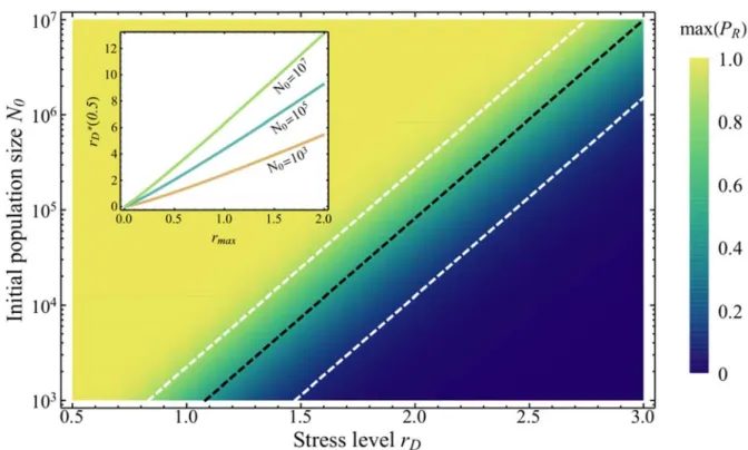
Figure 4 illustrates, for an initially clonal population, the sharpness of the transition from ER being 494
almost certain to being highly unlikely ( 1 to 0) as a function of and . It also shows 495
the accuracy of the approximation for ∗ in Eq.[7] (dashed black line corresponding to the right
496
hand side approximation of Eq.[7]), compared to its numerical estimation from Eq.[5] (color 497 gradient). Supplementary Figure 5 shows a similar result for a population starting with standing 498 genetic variance. 499 500
501
Figure 4: ER probabilities from de novo mutants only (Eq.[5]) for different values of and . The
502
color gradient gives the value of (see legend). The red straight line corresponds to
503
(Eq.[7]) and the black dashed line corresponds to ∗ 1 2⁄ (right hand side
504
approximation of Eq.[7]). For a given , the ER probability drops sharply from 1 (light yellow)
505
to 0 (blue), over a short increase in . For a given , rises sharply as increases about ∗
506
and then drops sharply as increases around . Other parameters are 1, 10
507
and 5 10 . 4 in panel (a) and 8 in panel (b).
508
509
The upper bound is independent of initial conditions or stochasticity, as lethal 510
mutagenesis depends on the deterministic equilibrium state of the population, once adapted to 511
the stress. Therefore, does not depend on the presence or absence of initial standing 512
variance, the decay rate imposed by the environmental change ( ) or the initial population 513
size . On the contrary, the lower bound ∗ depends on these factors as it is determined by the
514
capacity of the population to transiently adapt to the new conditions. It shows, however, little 515
dependence on dimensionality ( ), as is also apparent in Figure 4, by the accuracy of Eq.[7], which 516
is independent of . Overall, the width of the mutation window where ER is likely decreases with 517
increasing stress (Figure 4) and increases with initial population size (eq. [7]: ∗ decreases
518
with , and is unchanged). The width of the window decreases with dimensionality and 519
increases with the maximum fitness in the new environment , because both parameters affect 520
the upper bound of the window, (eq. [7]). Lower dimensionality and higher maximum 521
population growth rate reduce the mutation load, and thus allow persisting under higher mutation 522
rates. 523
Finally, note that we focused on the effect of here, but similar results could be obtained if was 524
varied (as both parameters affect as a product √ ). This is apparent in Eq.[7] where 525 and could be exchanged. 526 527 Height of the window and “Mutation proof extinction”: within the mutation window ( ∗ 528 ), the ER probability rises above 50% and then drops back to zero. Yet, for more extreme 529 stresses, it cannot even reach above 50% for any value of the mutation rate: the height of the 530 mutation window lies below 1/2). When this height is low, extinction is ‘mutation proof’, in that it 531
is highly likely whatever the mutation rate(s) or the variance of mutational effects in the 532
population. To illustrate this, we compute the maximum of the ER probability max when 533
varies from to , by numerically evaluating Eq.[5] over this range. Supplementary Figure 6 534
shows detailed profiles of ER probabilities against mutation rates (illustrating how max is 535
found), in the presence or absence of initial standing variance. Figure 5 shows the maximum 536
attainable as a function of and : it drops (transition from yellow to blue areas) with increasing 537
stress and decreasing population size . In this example, a large part of the combinations of 538
the two parameters and correspond to max lower than 10% (blue area below the lower 539
white dashed line in Figure 5). Therefore, for a given inoculum size , there is always a threshold 540
of stress level beyond which ER is nearly impossible, whatever the mutation rates in the population. 541
A closed form approximation can be obtained to describe this transition (detailed in 542
Appendix I section VII): denote ∗ the value of at which max for some ∈ 0,1 . 543
We obtain the following simple expression for the threshold of level of stress beyond 544
which max cannot exceed some level , independently of : 545 ∗ log log 1 1⁄ with ∶ 0.6 ∶ 0.31 , [8] where the values of come from a curve‐fitting procedure (detailed in Appendix I section VII). 546 Setting ≪ 1 in Eq.[8] thus provides the stress level beyond which ER is very unlikely, whatever 547
the mutation rate or the variance of mutational effects . This means, in particular, that the 548
evolution of higher mutation rates (via hypermutator strains) or higher variance of mutational 549 effects (larger ) would not allow the population to avoid extinction, when confronted to this stress 550 level. The validity of the heuristic in Eq. [8] is illustrated in Figure 5, where we see that the dashed 551
lines ( ∗ with 0.1,0.5,0.9 see legend) accurately predict the transition from high to low 552
values of max , computed numerically from Eq.[5]. 553
This whole argument applies to both and scenarios (by choosing 554
accordingly in Eq. [8]). Interestingly, we can also see that populations initially at mutation‐selection 555
balance (standing genetic variance) can withstand stresses twice larger than populations only 556 adapting from de novo mutations (initially clonal). 557 558 559
Figure 5: Maximum ER probability reached as is varied, for different values of and for a
560
population with no initial polymorphism. The color gradient gives the value of this time
561
(see legend). The black dashed line gives the value of ∗ 0.5 (Eq.[8] with 0.6) and the white
562
dashed lines the value of ∗ 0.1 and ∗ 0.9 . The maximum of the ER probability attainable (for
563
all possible ) drops sharply over a short range of increasing for a given , or over a short range
of decreasing for a given . Other parameters are 0.5, 4, and 5 10 . The
565
inset panel shows how ∗ 0.5 from Eq.[8] varies with and .
566
567
Distribution of extinction times: From Eq.[4] we can derive the probability density of this
568 distribution, in either of the two scenarios considered (purely clonal population or population 569 at mutation‐selection balance ). We get: 570 ∞ 2 ∞ / exp 2 , [9]
where the functions . and . depend on the scenario considered and are given explicitly in 571
Eq.[5]. Figure 6 illustrates the accuracy of this result and how the distribution of extinction times 572
varies with stress intensity and mutation rate . In spite of neglecting evolutionary stochasticity, 573
Eq.[9] still captures the shape and scale of extinction time distributions, in the WSSM regime. 574
575 Figure 6: Density of the extinction probability dynamics for different values of (panel (a) and (c)) 576 and (panel (b)). The distributions of extinction times from simulations started with an isogenic 577 population are shown by shaded histograms, with the corresponding theory (Eq.[9]) given by the 578
plain red lines. The color gradient corresponds to increasing levels of (panel (b)) or of (lower
579
range in panel (a) and higher range in panel (c), as indicated on the legend). Each simulated
580
distributions is drawn from 1000 extinct populations among a sufficient number of replicates to
581
observe these 1000 extinctions. The mutation rates covered in panel (a) are
582
0; 4 ; 8 ; 14 and in panel (c) are 2 ; 1.5 ; 1.1 and in both panel
583
the decay rate is 0.28. The decay rate covered in panel (b) are 0.285; 0.33; 0.4; 0.5 and the
584
mutation rate is 15 . Other parameters are 10 , 4, 0.1 and
585 5 10 . 586 587 Figure 6b shows that decreasing the stress level ( ) increases the mean persistence time 588 of the population and also increases the variance of this duration. This behavior could be seen as 589
a mere scaling: even in the absence of evolution the population takes longer time to become 590
extinct with a smaller . On the contrary, increasing the mutation rate, keeping it below the lethal 591
mutagenesis threshold (0 , Figure 6a), increases the mean and the variance of the 592
persistence time. This likely stems from subcritical mutations (0 , beneficial but not 593 resistant) that can transiently invade the population, thus delaying its extinction. However, beyond 594 the lethal mutagenesis threshold ( , Figure 6c), the trend is reversed: extinctions (which 595 are always certain then) occur faster at high mutation rates (panel c). Therefore, even in those 596
cases where ER probabilities are uninformative ( 0), the distribution of extinction times 597 conveys important information on the underlying adaptive or maladaptive dynamics.
598
599
Discussion
600We investigated the effect of an abrupt environmental change on the persistence of 601 asexual populations with a large mutational input of genetic variance (WSSM regime), adapting 602 either from de novo mutations arising after the environmental change ( scenario) or from both 603 de novo and pre‐existing mutations ( scenario). In a previous study (Anciaux et al. 2018), 604 we studied evolutionary rescue when considering adaptation over a phenotype‐fitness landscape 605 (FGM), which implies pervasive epistasis between multiple mutations and imposes a relationship 606
between the initial decay rate of the population, the proportion and growth rate of resistance 607
alleles, and their selective cost in the ancestral (before the stress) environment. However, we 608
assumed that rescue resulted from rare mutations with strong effects (SSWM). The key 609
contributions of the present model, building on our previous work, are to (i) allow for the 610 cumulative effect of multiple mutations and (ii) provide insights into the distribution of extinction 611 times in the presence of an evolutionary response. 612 613 Single step (SSWM regime) vs. multiple step (WSSM) regimes in ER: In spite of its complexity, the ER 614 process in high mutation rate regimes can readily be captured by simple analytic approximations 615
(Eqs.[5] and [6]), which neglect evolutionary stochasticity and only account for demographic 616
stochasticity. Overall, the SSWM and WSSM approximations roughly capture the ER process in 617
complementary domains of the mutation rate spectrum (Figures 1‐3). 618
This approach shows how multiple mutations allow withstanding higher stress than what 619
the single step approximation (SSWM in Anciaux et al. 2018) predicts (Figures 1 and 3). However, 620
this is only true for intermediate mutation rates: a further increase in mutation rate ultimately 621 shifts the system to a lethal mutagenesis regime (Figures 2 to 4). Indeed, the dependence between 622 the ER probability and the mutation rate is not monotonic. The model shows an optimal mutation 623 rate for the ER probability, at which the maximal ER probability may be less than 1 (depending on 624 the stress, Figure 5). Beyond this rate, the ER probability drops down, to some point ( , Eq. [7]) 625 where the mutation load is so large that absolute fitness is negative at mutation selection balance. 626 This non‐monotonic dependence reflects the continuum between ER and lethal mutagenesis along 627 a gradient of mutation rates. 628 629 Similarities to existing ER models: Some of our key previous findings (Anciaux et al. 2018), regarding 630 how ER depends on the parameters of the fitness landscape (FGM here) are still valid in the more 631
polymorphic WSSM regime. The main common features are (i) the sharp decrease of ER 632
probabilities with stress (decay rate ), (ii) their log‐linear increase with initial population size , 633
(iii) the fact that standing variance allows withstanding higher stress, (vi) the limited effect of 634
dimensionality (for mutation rates far from lethal mutagenesis, eq. [6]). The effect of initial 635
population size ( 1 exp eq.[5]) is exactly the same as in previous models where ER 636
stemmed from single mutants (SSWM regime Orr and Unckless 2008, 2014; Martin et al. 2013; 637
Anciaux et al. 2018). This is expected of any model ignoring interactions between individuals, be it 638
evolutionary (e.g. sexual reproduction or frequency‐dependent selection) or demographic (e.g. 639
density‐dependence): each of the lineages initially present contributes independently to ER 640 (with some rate per individual). Decay rate has a broadly similar (but quantitatively different) 641 effect in previous ER models not based on a fitness landscape. The other parameters ( , , ) 642 are not defined outside the FGM. More generally, the key implications of considering the FGM to 643 model ER are detailed more thoroughly in Anciaux et al. (2018). 644 645


![Figure 4: ER probabilities from de novo mutants only (Eq.[5]) for different values of and . The 502](https://thumb-eu.123doks.com/thumbv2/123doknet/13481150.413381/24.892.128.768.154.408/figure-probabilities-from-novo-mutants-only-different-values.webp)