Data-driven models for reliability prognostics of gas turbines

Data-Driven Models for Reliability Prognostics of

Gas Turbines

by

Gaurev

Kumar

Submitted to the The Center for Computational Engineering

in partial fulfillment of the requirements for the degree of

Master of Science in Computation for Design and Optimization

at the

MASSACHUSETTS INSTITUTE OF TECHNOLOGY

June 2015

@

Massachusetts Institute of Technology 2015. All rights reserved.

Author...

Certified by...

Signature redacted

The Certr for Computational Engineering

May 18, 2015

Signature redacted

Saurabh Amin

Assistant Professor, Civil & Environmental Engineering

Thesis Supervisor

AcceDted by ...

Signature redacted

N

as Hadjiconstantinou

Professor, M hanical Engineering

Co-Director, Computation for Design and Optimization

Co-Director, Computational Science and Engineering

ARCHINES

MASSACFHUSETTS INSTITUTEOF

TECHNOLOGY-OCT 212015

Data-Driven Models for Reliability Prognostics of Gas

Turbines

by

Gaurev Kumar

Submitted to the The Center for Computational Engineering on May 18, 2015, in partial fulfillment of the

requirements for the degree of

Master of Science in Computation for Design and Optimization

Abstract

This thesis develops three data-driven models of a commercially operating gas turbine, and applies inference techniques for reliability prognostics. The models focus on capturing feature signals (continuous state) and operating modes (discrete state) that are representative of the remaining useful life of the solid welded rotor. The first model derives its structure from a non-Bayesian parametric hidden Markov model. The second and third models are based on Bayesian nonparametric methods, namely the hierarchical Dirchlet process, and can be viewed as extensions of the first model. For all three approaches, the model structure is first prescribed, parameter estimation procedures are then discussed, and lastly validation and prediction results are pre-sented, using proposed degradation metrics. All three models are trained using five years of data, and prediction algorithms are tested on a sixth year of data. Results indicate that model 3 is superior, since it is able to detect new operating modes, which the other models fail to do.

The turbine is based on a sequential combustion design and operates in the 50Hz wholesale electricity market. The rotor is the most critical asset of the machine and is subject to nonlinear loadings induced from three sources: i) day-to-day variations in total power generated by the turbine; ii) machine trips in high and low loading conditions; iii) downtimes due to scheduled maintenance and inspection events. These sources naturally lead to dynamics, where random (resp. forced) transitions occur due to switching in the operating mode (resp. trip and/or maintenance events). The degradation of the rotor is modeled by measuring the abnormality witnessed by the cooling air temperature within different modes. Generation companies can utilize these indicators for making strategic decisions such as maintenance scheduling and

generation planning.

Thesis Supervisor: Saurabh Amin

Acknowledgments

Firstly, I would like to thank my advisor, Dr. Saurabh Amin for all of his support, guidance, and patience throughout my time at MIT. Our weekly discussions-those

about mathematics and those not-will always be cherished.

I would like to also thank the Accenture and MIT Alliance in Business Analytics for

their financial support for conducting this research. Collaborating with the entire

Accenture team was very instructive and helpful. I would like to also thank the

electric-ity production company which provided the data, allowing for analysis and simulations.

Finally, I would like to thank my mother, father, and entire family for always believing

in me and encouraging me to strive for perfection, both of craft and mind.

Data analysis and simulations in this thesis were made possible by computational

Contents

1 Introduction 9

1.1 Gas Turbine Overview . . . . 10

1.1.1 Developing a GT Model ... 11

1.1.2 Intra-Modal Dynamics ... 12

1.1.3 Inter-Modal Transitions . . . . 13

1.2 Gas Turbine Reliability . . . . 13

1.2.1 Operation Concept . . . . 13

1.2.2 Rotor Degradation . . . . 14

1.3 Related Work . . . . 17

1.4 Contributions & Outline . . . . 18

2 Parametric & Nonparametric Models 22 2.1 Background . . . . 22

2.1.1 Probability Distributions . . . . 22

2.1.2 Mixture Model . . . . 25

2.2 Parametric Models . . . . 26

2.2.1 Finite Hidden Markov Model . . . . 26

2.2.2 hidden Semi-Markov Model . . . . 28

2.3 Nonparametric Models . . . . 29

2.3.1 Dirichlet Process . . . . 29

2.3.2 Hierarchical Dirichlet Process . . . . 32

2.3.3 HDP-HMM . . . . 35

2.4.1 Weak Limit Approximation . . . . . . 37

40

. . . . 43

. . . . 44

. . . . 47

3 Non-Bayesian Parametric Model

3.1 Power Output Detrending . . . .

3.2 Degradation Model . . . .

3.2.1 Forced JUi.ps . . . .

4 Two Bayesian Nonparametric Models

4.1 IDP-IHSMM . . . . 4.2 HJDP-SLDS-HMM . . . . 5 Reliability Prognostics 5.1 Deterioration Metrics . . 5.2 Model Validation... 5.3 Deterioration Results . 5.4 HDP-SLDS-HMM Results 5.5 Prognostics . . . . 6 Concluding Remarks

. . . .

. . . .

. . . .

. . . .

. . . .

List of Figures

1-1 Gas turbine components . . . . 11

1-2 GT operation concept . . . . 15

2-1 Hidden Markov Model . . . . 27

2-2 Hidden Semi-Markov Model . . . . 30

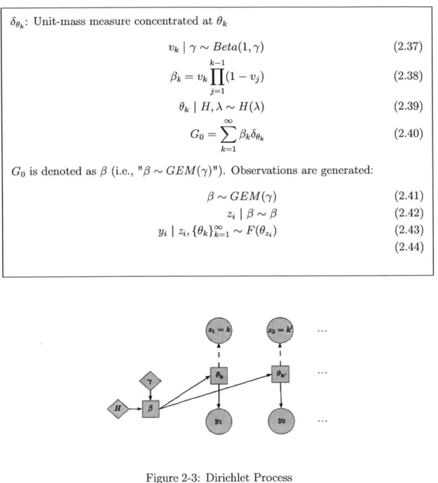
2-3 Dirichlet Process . . . . 32

2-4 Hierarchical Dirichlet Process . . . . 34

3-1 Three types of intra-day power-output signals . . . . 41

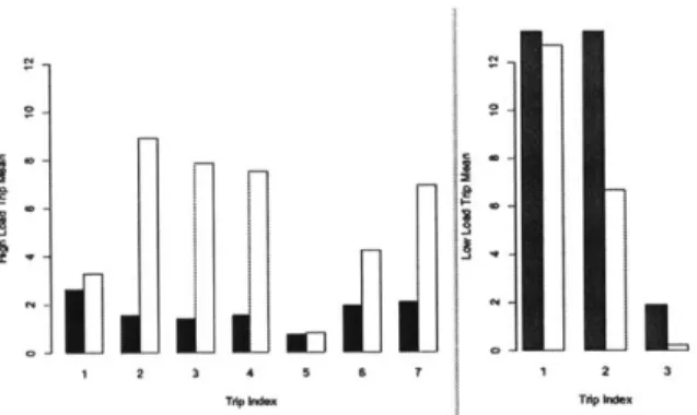
3-2 Example of g(-). Left set corresponds to High Load Trips. Right set to Low Load Frips. g(.) is the mean of the TAT signal, 2 hours before the trip. Red,/ Blue=Trip, White=Normal. . . . . 48

4-1 IDP-1ISM M . . . . 50

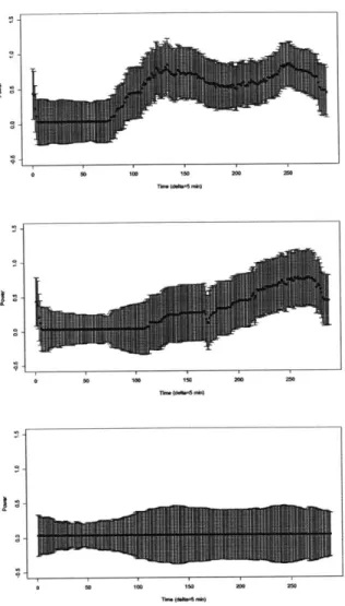
5-1 Mean power signature, with .5 standard deviation bands . . . . 56

5-2 Model 1,2,3 fitted models for cooling air temperature across first 5 years 57 5-3 OM classification: Normal=Light Grey; Semi-Normal=White; Abnor-mal=Dark Grey; Other= Black . . . . 58

5-4 Evolution of Rotor Temperature, Ds, 1K , Cumulative Sum of D. across all 5 years (all graphs are subsampled every 10 days) . . . . 59

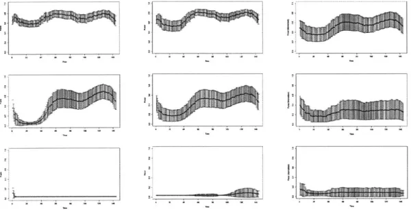
5-5 HDP-SLDS-HMM OM mean power signatures (left column) with corre-sponding mean cooling temperature (right column) . . . . 63

5-6 Fitted NBP-HDMM regression model (panel l'; D, (panel 2); Cumulative

Sum of D, (panel 3); Viterbi OM classification dwell percentages for

the sixth year (panel 4) (subsampled every 10 days) . . . . 64

5-7 Predicted temperature time series using method 1 (panel 1); predictions using method 2 (panel 2); comparison of mean absolute errors (panel

List of Tables

Chapter 1

Introduction

In this thesis, three probabilistic reliability modeling approaches are presented. The

structures of all three models are discussed and their practical applications are

an-alyzed using data from gas turbine (GT) assets. Although the focus in this thesis

is GT-centric, the models are general enough to be applicable to other dynamical

systems. The first model is non-Bayesian parametric (NBP) and the remaining two are

Bayesian nonparametric (HDP). Results from the three approaches will be discussed

and compared.

The models are developed for a real-world GT operating according to the Brayton

thermodynamic cycle. The GT forms the part of a commercially operating Combined

Cycle Gas Turbine (CCGT) plant, where the hot exhaust from the GT is used to

power a steam power plant (operating according to the Rankine cycle). The CCGT

operates in the 50 Hz wholesale electricity market, and is a part of the generation

fleet of a large electricity producer in Europe. The electricity producer (i.e., the

GenCo) continuously collects data from sensors and controllers that are embedded

in the GT for the purpose of performance monitoring, maintenance scheduling, and

generation planning. In particular, the data provided is a continuous stream of data

from 153 sensor-control signals at 5 min intervals for a period of six years (2009-2014).

that are indicative of the condition of GT's rotor, which is the most critical fixed asset of the machine. The day-to-day dynamics are modeled as random switches between a fixed number of operating modes (OMs), and are assumed to be generated from a discrete-time stochastic process. The intra-day dynamics of the asset's condition is assumed to evolve according to a linear regression model, dependent on the day's

OM for NBP-HMM (model 1) and HDP-HSMM (model 2). In contrast, for the HDP-SLDS-HMM (model 3), the emission structure imbeds the regression model directly. Thus, the system can be viewed as a hierarchy, with each level observing dynamics with a different structure.

1.1

Gas

Turbine Overview

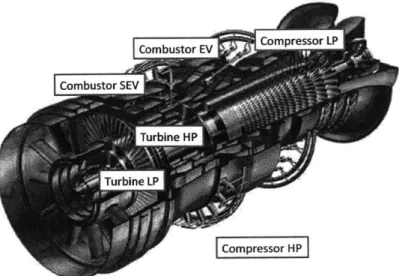
Gas turbines are internal combustion engines that are heavily relied upon to generate mechanical energy with chemical energy inputs. A typical gas turbine has five stan-dard components: inlet, compressor, diffuser, combustor, and turbine (with exhaust). Figure 1-1 presents a schematic of the GT used in this study. Gas turbines produce two streams of energy. The first energy stream is used to power an output shaft, while the second stream is used by the gas turbine, itself, to power the compressor. Gas turbines can be viewed as partially self-sustaining in that part of the energy produced is recycled to power internal components.

The process by which gas turbines generate energy can be viewed as a cycle which converts gaseous energy into mechanical energy. Large amounts of clean, unimpeded airflow is provided to the gas turbine by the air inlet. This air, which initially has atmospheric pressure is then converted into high-pressure air. With multiple stages of rotor blades and stator vanes, the compressor incrementally increases the impact pressure (velocity) of the supplied air. The diffuser, through its divergent duct design converts most of the impact pressure of the air output from the compressor into static pressure air. This low velocity, high static pressure air enters the combustor which burns the fuel-air mixture, while the cooling system and liners keep parts safe from the

Figure 1-1: Gas turbine components

high flame temperatures produced from the combustion. The gaseous mixture is then

run through a convergent duct which accelerates the gas, reducing the static pressure,

as well as decreasing the temperature to feed into the turbine. The turbine has the

"reverse" deign of the compressor, in that it extracts mechanical energy from the

gaseous energy to drive the output shaft, and feeds power back into the compressor.

After the gas has passed through the turbine, it exits through the exhaust [1].

The Brayton cycle summarizes the main thermodynamic processes that take place

in a gas turbine. It begins with adiabatic compression in the inlet and compressor,

followed by constant pressure fuel combustion. This is followed by adiabatic expansion

in the turbine, with which some force is taken out of the air to drive the compressor,

after which the remaining force is used to accelerate the output shaft. Finally, the

cooling of the air at constant pressure returns the cycle to its initial condition [2].

1.1.1

Developing a GT Model

We would like to construct a model for the evolution of the degradation proxy signals

by defining the dependency on observed feature signals and mode transitions. Because

observe how long the rotor stays "healthy" before it drops below a certain degradation

threshold. Instead we must infer, from the features (i.e. observable signals) that are

correlated with the degradation of the rotor, how the dynamics of degradation of the

rotor are changing. The data is obtained from sensors placed in various locations

inside and in the ambient areas outside of the turbine. The sensors capture four

types of readings: pressure, power, vibration, and temperature. The data can be

organized in three buckets: process, refrigeration, and vibration. Process data refers

to data collected by sensors on parts of components which are critical to maintaining

thermodynamic parameters so that the turbine is working efficiently. Refrigeration

data comes from sensors which are placed in ducts/ cavities in which cooling air

passes through for neutralizing high temperatures generated by certain processes. And, vibration data is collected by sensors which measure movements of components in

units of mm/s.

1.1.2

Intra-Modal Dynamics

The gas turbine Operation Concept (OC) dictates the governance of temperature and

mass air flow of gas turbine, as a function of power output, using limit points. Because

the OC is idealized, and not observed in practice, it allows us to define a distance

metric characterizing how 'far' the systems operating conditions for a given period are

from the idealized. More importantly, it induces a mapping from a particular operating

condition to a particular operating mode (OM). At any given time, the system resides

in a particular mode, completely characterizing the operating performance of the

system at that time.

These operating conditions have a direct impact on the dynamics of the

observ-able features that relate to the health state of the rotor, and by extension the evolution

1.1.3

Inter-Modal Transitions

We can view the GT system as one which dwells and transitions between finitely many

OMs. The system dwells in exactly one state at any given time and it can transition

from one state to another when a trigger condition is satisfied, based on the active

transition law/kernel at any given time. As stated above, there exists a correspondence

between the OMs and the operating condition of gas turbine. The transition law

between different operating conditions must accommodate non-autonomous, as well

as autonomous/stochastic transitions.

The system may transition between different operating conditions autonomously

based on some probability distribution, as well as non-autonomously due to forced

transitions that may occur because the state of the system (i.e. specific observed

signals) reaches a pre-specified abnormal threshold, or due to a planned event that

must take place a pre-specified time, which triggers a jump. We can define the

transition law which causes the switches between modes as a Markov process.

1.2

Gas Turbine Reliability

The GT is governed by an operation concept (OC), which dictates how the machine

should ideally perform its startups, normal operation, and shutdowns sequences.

Degradation of the machine can be viewed as occurring when the machine operates in

conditions that are very different from the OC.

1.2.1

Operation Concept

The machine is fired up when the first combustor, called the Environmental (EV)

com-bustor, starts its operation. Pilot flames are used in the EV burners for initiating the

combustion of fuel (gas) mixed with air. At 20 % of base load, the EV burners switch

to premix operation, and a second combustor, called the Sequential Environmental

opened, and more fuel is supplied to the two combustors. The exhaust temperature of

the turbine is kept constant by controllers, until full load is reached. This is achieved

by means of a small increase in the combustor temperature with the VIGV fully open.

Optimal operating conditions of the EV burners range from 25 % load to the full load.

The EV combustor is an annular combustion chamber with 30 burners. Combustion air

enters the cone through air inlet slots while the fuel is injected through a series of fine

holes in the supply pipe. The gaseous pilot fuel and the liquid fuel are injected through

nozzles at the cone tip. This ensures that the fuel and air spiral into a vortex form

and are mixed. The annular design provides an even temperature profile, resulting in

improved cooling, longer blade life and lower emissions. The SEV combustor consists

of 24 diffusor-burner assemblies, followed by a single, annular combustion chamber

surrounded by convection-cooled walls. The exhaust gas from the high-pressure (HP)

turbine enters the SEV combustor through the diffusor area. Due to the elevated

temperatures of the HP turbine exhaust, the fuel-air mixture ignites autonomously.

Finally, the low-pressure (LP) turbine operates at the tail end of the machine.

As the GT transitions from minimum-load to part-load to base load levels, various

temperature limits are utilized in order to actuate appropriate controls to maintain

GT efficiency and performance levels. These temperature limits are defined by the

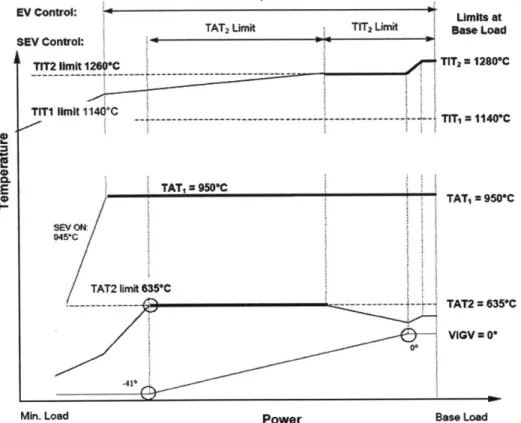
OC of the GT; see Fig. 1-2 where these limits are denoted TIT, TIT2, TAT, and

TAT2. Essentially, these limits are the ideal levels of the aggregate temperatures of different subcomponents of the machine as a function of the power loading.

1.2.2

Rotor Degradation

As the GT gets older, most components begin to show signs of degradation.

Under-standing the degradation patterns of parts which are not easily replaceable-such as

the rotor shaft-is of crucial importance, because they tend to be the most integral

and expensive components. The principal components of a rotor are the shaft, disk, bearings, and seals. The bearings support the rotating components of the system and

TAT, LMit

Limits at i~d2~fl5I~mu BSLO

]AT2 Limt Baft Load

SEV Control:

TfT2 -lmit 12 TI_ 1Ta=12SC

TIrTrI lmit 114 C _{--- - --- TIT,} 114W*C TATI x5C ___ TAT =95VC SEV ON: TAT2 Im*it635*C --- --- TAT2 6350C VIGV =0* 0*

Power Base Load

Figure 1-2: GT operation concept

EV Control:

e

Z

CL

stabilize the rotor vibration, while the seals prevent undesired leakage flows inside the machines of the processing or lubricating fluids [3].

Rotors can begin to degrade in many ways. The condition of the rotor is dependent

on two major factors: creep and low-cycle fatigue (LCF). Due to constant loads, there

is a risk of creep, which manifests itself in the propagation of cracks within the rotor.

When the temperatures pass a certain percentage of the melting point of the material,

the probability of creep is high. Furthermore, high temperature gradients, caused by

poor casing insulation can lead to elastic rotor bending.

Additionally, LCF accelerates the degradation of the rotor, when it must undergo

high amplitude, low frequency strains. This occurs mainly when the system is turned

on and shut down multiple times in a short period of time [3]. The rapid switching

between different electricity production levels shifts the rotation axis of the shaft by

moving the mass center of the rotor. This leads to an increase in rotor vibration [4].

In addition to LCF, long exposure to high levels of mechanical stresses cause rotor

shaft deterioration due to creep deformation. Creep also initiates cracks on the surface

of the rotor. Under high temperature and pressure loadings that are typical of a GT,

risk of creep induced deterioration increases. When the temperature surrounding the

rotor surpasses 40 % of the melting point of the rotor, the probability of creep is

especially high

12].

Rotor degradation dynamics are tied to the different OMs because the behavior of the

GT varies drastically under different OMs. Dynamics of the rotor temperature signal

differs when the system dwells in different OMs, and change depending on how the

turbine transitions between each of these OMs. Specifically, as the turbine transitions

from periods of normal operation characterized by loads of approximately 400 MW,

dynamics of temperature that the rotor faces change. Thus, we can view the rotor

temperature, as a time-evolving signal, whose dynamics are governed by the OM in

which it dwells.

The mechanistic models of creep and LCF indicate that the variability of loads

(stresses) and temperatures in various OMs contribute to progressive deterioration. In

our work, random switching rates between the OMs are indicative of the variability in

loads on GT. To determine the modes and mode-switching rates, the power output

signal from the GT is used. To model the intra-day dynamics, the temperature of the

cooling air that circulates in the ducts around the rotor is chosen as the proxy of the

rotor temperature.

1.3

Related Work

Many publications have proposed various data-driven methods for estimating

degra-dation trajectories of various subsystems within gas turbines. Yet, past research

has dealt mostly with health state trajectory estimation of compressor blades and

bearings. Statistical methods such as Monte Carlo, HMMs, neural networks, Gaussian

mixture models, and various artificial intelligence methods using fuzzy logic have

been used for estimation and prediction purposes [4,51. Venturini et. al presented a

prognostic methodology, which estimates remaining useful life of GTs using statistical

techniques, by estimating the propensity of a turbine to transition from an "operable"

to "inoperable" state [5]. By sampling the intervals of time that the turbine remained

in any one of these states, Weibull distributions are generated, from which simulations

are conducted to compute the probability of dwelling in the operable mode. In contrast, the methods we describe automatically learns the number of OMs, without having to

a priori posit a number of states. This allows for model flexibility.

The transition matrix/kernel, which governs how OMs switch among one another

Since the OMs in which the GT dwells are tied to random fluctuations induced by

the bulk electricity market, we posit a model in which the OMs switch according to a

probabilistic relation. This facet has been explored in existing literature which apply

Piecewise Deterministic Markov Processes (PDMPs) for reliability prognostics [7,8,9].

Davis introduced as the most general class of continuous-time Markov processes which

include both discrete valued and continuous valued processes, except diffusion [7]. A

PDMP consists of two components: a discrete component and a continuous component.

Here, the OMs take discrete values and the rotor temperature is the continuous valued

solution of a OM-dependent difference equation. At discrete moments in time, the

discrete valued component may switch or jump to according to specified relation.

Numerous system identification methods are also available for parameter estimation of

intra-OM models [10,11]. Morari et al. propose a method of identifying hybrid systems

that are assumed to be piecewise affine (PWA). In this case, the OMs map to a finite

sequence of polyhedra which partition the space in which the continuous variable take

values [10]. Within each of these polyhedra, an affine difference equation governs

the evolution path of the continuous variable. And, the transition law is completely

determined by the system reaching the boundary of the polyhedra. The algorithm

that Morari et al. proposes makes use of support vector machines, and clustering

in order to estimate the intra-OM models and the transition law (boundaries of the

polyhedra).

1.4

Contributions & Outline

The pragmatic goal of this work is to understand both modeling approaches (NBP

and HDP) and comment on how both differ in estimation and prediction power of

the condition of critical assets (e.g., rotors, stators, casings) of large machines such as

gas turbines, steam turbines, and generators. The operational flexibility of GenCos can be significantly affected if they have limited visibility on the rate at which their critical assets are deteriorating. In recent years, GenCos world-wide are developing

a sense of urgency toward prognostic assessment of their generation fleet. The main

reason of this urgency is the fact that although the frequency of complete failure of

critical assets might be quite low, their replacement costs and delivery times can range

from months to years. Ignoring the early indicators of deterioration can lead to huge

unexpected economic losses. Moreover, if a large-side generation unit faces disruption

due to a failure of a critical asset, the GenCo may even loose its strategic position in

the competitive wholesale market.

Especially important is to be able to account for the supply-demand shocks and

non-stationarity in production trends [1]. For example, the power plants are expected

to have the capability to execute quicker start-up times and switch between one

operating point to another when another generator trips and creates a sudden loss

of supply. The push for flexible ramp-up and ramp-down schedules is even higher in

markets that are gradually accommodating new renewable energy sources. Additional

impositions on large machines such as compliance with environmental standards (e.g., cap on emissions) will make their future operating environment even more stringent.

Thus, we expect that the machines' critical assets will be subject to new loadings and

new temperature and pressure variations. This, in turn, will directly effect their rate

of deterioration. Due to the aforementioned reasons, utilizing the available data for

building accurate dynamical models of deterioration indicators (i.e., the condition) is

an important task, as confirmed by many business leaders in large-scale electricity

production [1].

Previous work in modeling deterioration of machine components has primarily focused

on replaceable components (e.g., blades within turbine's compressors) [4, 51. Since

these components have shorter lifetimes, the available condition monitoring data

can capture their deterioration rates, starting from the time of their installation to

the time of their replacement. Major GT manufacturers (e.g., Alstom, GE Energy, Siemens, United Technologies) are fairly specific in recommending the maintenance

components such as rotor shaft is not straightforward, as they typically have much

longer lifetimes (20-30 years). Hence, data on their actual failure rates is not readily

available. GT manufacturers conduct laboratory tests on these assets during design

phase, but there is no direct way to conduct tests on these assets once they are

installed in an operational machine. Thus, currently there is no practical procedure to

estimate the remaining useful life (RUL) of GT rotors.

In chapter 2, we present necessary background on the three models that we will be

presenting. The chapter begins with a brief overview of probability distributions

and mixture models, followed by structures of parametric and nonparametric

hid-den Markov models (HMM). In chapter 3, we present the non-Bayesian parametric

HMM for rotor degradation. A new detrending method is presented that allows for

dimensionality reduction of the HMM emission variable. In chapter 4, we present

two Bayesian nonparametric models. The first model is a semi-Markov model, and

is able to estimate dwell times in different operating modes, using the exponential

distribution. The second model uses an Switching Linear Dynamical System (SLDS)

emissions model, which is able provide a richer model structure. In chapter 5, we

posit metrics for degradation that are later used to validate all three models, and

compare performance. Calculations and comparisons of the cumulative deterioration

estimated over the time are presented. The chapter concludes with a discussion of

different prediction algorithms, which are tested on the sixth year of data. Finally,

concluding remarks end the thesis in chapter 6.

The main contributions of this thesis are the three models. Model 1 is the parametric

non-Bayesian hidden Markov model (NBP-HMM). In model 1, each day is classified

as an operating mode (OM) by the HMM with a detrended intra-day power signal

as the emission. For this model, the number of OMs is assumed to be 3. Model 2

is the nonparametric Bayesian hidden semi-Markov model (HDP-HSMM). In model

2, each day is classified as an operating mode (OM), but the emissions are now the

the number of OMs learned by the model itself, utilizing an imbedded Dirichlet process.

For models 1 and 2, once the OMs are learned, a linear regression model is fit for

the cooling air temperature signal, for each OM. Using the residuals from the fitted

regression model, deterioration levels are estimated.

Model 3 is the nonparametric Bayesian HMM with a switching linear dynamical

system emission model (HDP-SLDS-HMM). In model 3, each day is classified as an

operating mode (OM), but the SLDS emission structure allows for simultaneous fitting

of intra-day temperature signal. Thus, the regression model is not needed to estimate

Chapter 2

Parametric & Nonparametric Models

2.1

Background

This chapter begins by describing common probability distributions that will be

used as basic building blocks for the models that we consider in this thesis. This

is followed by descriptions of more complex probabilistic graphical models that will

ultimately be tailored specifically for the application of GT reliability. For all of

the models described, both Bayesian and non-Bayesian forms exist. In a Bayesian

framework, appropriate prior distributions are placed on model parameters, while in a

non-Bayesian framework, parameters are assumed to be fixed.

2.. . rXJLaicLiUy JuDstIibU tiosU11b

A. Categorical

The categorical distribution is a generalization of the Bernoulli distribution, and is

also called a "discrete distribution" [17]. It is a distribution that describes the result

of a random event that can take on one of k possible outcomes, with the probability

of each outcome separately specified. If x is a random variable distributed categorical, with parameters (Pi, ... ,pA), such that E~ pi = 1, then x E {1, . . ., k}

k

p) = pX=i] (2.1)

i=1 Here, [x = i] denotes the Iverson bracket, where

[x

oteri

B. Binomial/ Multinomial

The binomial distribution is the distribution governing the number of successes for one of just two categories in n independent Bernoulli trials, with the same probability of success on each trial [17]. The multinomial distribution is the generalization of the binomial distribution, where each trial results in exactly one of some fixed finite number k possible outcomes, with probabilities (p1, ... ,Pk), such that i=1 pi = 1. If the random variables xi indicate the number of times outcome number i is observed over the n trials, the vector x = (X1,..., Xk) follows a multinomial distribution with parameters n and p, where p = (P1,. .. ,Pk), where

k

p(x) = p(X,

.!

..! ,k)ip

(2.3)

If n = 1, the categorical distribution is obtained.

C. Dirichlet

The Dirichlet distribution is a family of continuous multivariate probability dis-tributions parameterized by a vector of positive reals [131. It is the multivariate generalization of the beta distribution. Dirichlet distributions are very often used as prior distributions in Bayesian statistics, and is the conjugate prior of the categorical distribution and multinomial distribution. The Dirichlet distribution of order k > 2

with parameters a = (ai, ..., aK) > 0 has the following probability density function

I k

-f(x) = f(i,.. ., X) =

B>

(2.4)

Here, B(a) is the multinomial beta function, which is expressed through the gamma function as

B~a)

B(

=)1

(=)

(2.5)

]p'(Ek_1 Cei)

The infinite-dimensional generalization of the Dirichlet distribution is the Dirichlet process, which will be described in more detail later in this chapter.

D. Multivariate Gaussian

The multivariate Gaussian distribution is a generalization of the univariate Gaussian distribution [17]. The multivariate Gaussian distribution is said to be "non-degenerate"

when the symmetric covariance matrix E is positive definite. In this case, the k-dimensional a Gaussian-distributed random variable x = (xi,... ,x) with mean

vector p and covariance E has probability density

1 (1

f(x) = f(X1, xk) = exp I--(X - )E-1 (X - i) (2.6)

,/(27r)kII 2

E. Exponential

The exponential distribution is the probability distribution that describes the

inter-arrival time between different events in a Poisson process. The Poisson process is a stochastic process in which events occur independently at the same average rate [17]. It is the continuous analog of the geometric distribution, and is notedly memoryless. The probability density function (pdf) of an exponential distribution is

f(x; A)

Ae

2.1.2

Mixture Model

A mixture model is best explained by thinking about a system from which taking

measurements is a simple procedure [131. In some cases, the state of the system, at the time when the measurement is taken is known. Yet, for real-world systems, which are complex, the state of the system is usually unknown. Given a sequence

of measurements {yi, Y2, .. -, YN}, a mixture model posits that the data points are

sampled from a finite (or countably infinite) mixture of unobserved states z taking

values in K = {1, 2,... , K}. In the case of parametric/finite mixture models, the

cardinality of K is assumed known. In the case of nonparametric mixture models, the theoretical cardinality is assumed to be countably infinite, yet empirically a finite

number of states will exist. Because the states are unobserved, the data points

are used to infer two major qualities of the system. Firstly, each observation is

modeled as a random variable, with an underlying distribution coupled with a unique

state. Thus, given the observations, parameters governing the underlying distribution

can be inferred. And, secondly, the mixture model assumes a prior on the relative

importance of each state, which must be inferred, as well. Finally, given knowledge

of an observations generating state, the data are assumed to be independent. The

exhibit below outlines a Bayesian parametric mixture model.

Bayesian Parametric Mixture Model

K: Number of states (mixture components) {zi,. . ., ZN} K {1, ... , K}

N: Number of measurements {Y,... YN} E Rn

F: Probability distribution governing observation yi

Ok: Parameter governing distribution of observations emitted from kth state

8k: Mixture weight for kth state. B = (i3, ... , 6K) A: Hyper-parameter governing prior distribution of B

H(-y): Prior distribution with hyper-parameter of 0

k for all k E E

2.2

Parametric Models

2.2.1

Finite Hidden Markov Model

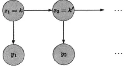
The hidden Markov model (HMM) prescribes a probability distribution over a sequence of observations [13]. The first assumption of the model is that the sequence of observations yt are sampled at discrete times t C

{1,

p r ocs, o 0- nam L. ely

P(Yt

I

I

With these four assumptions, we can write the joint probability distribution as

T

p(Y1:T, Z1:T) = p(z1)p(y1

I

I

With the model specified, the goal is to use data to infer the parameters of the HMM. The parameters are a triple {F, ir, ~ro}, the emissions distribution parameters (i.e,

Ok ~ H(7) (2.8) B ~ Dirichlet(A) (2.9) zi ~ Categorical(B) (2.10) yi zi = k ~ F(Ok) (2.11) Z0k=l1 ;#>kOVkEk (2.12) k (2.13)

{pk,

matrix governing the hidden process dynamics, and the initial distribution for the

hidden process, respectively. The exhibit below outlines a Bayesian parametric hidden

Markov model.

I

I

Figure 2-1: Hidden Markov Model

Bayesian Parametric Hidden Markov Model

K: Number of states (mixture components) {z1, .. . , ZT} E K = {1, ... , K}

(1, ... , T): Sequence of measurements {yi,... yT} E Rn

F: Probability distribution governing observation yt

Ok: Parameter governing distribution of observations emitted from kth state

irOk: Initial probability of kth state. ro = (iroi,... rOK)

irk: Transition probability distribution of state k. ik = (irkl, -,kK)

A: Hyper-parameter governing prior distribution of B

H(-y): Prior distribution with hyper-parameter of Ok for all k E K

Ok ~ H(-f) (2.16)

irk, _rO ~ Dirichlet(A) (2.17)

Z1 I iro ~ -ro (2.18) zt I zt_1 = k ~ rk (2.19) yt I zt = k - F(k) (2.20) rok = 1; frok

> 0 V k E

0 V j E

2.2.2

Hidden Semi-Markov Model

Although the parametric HMM is capable of modeling a variety of data structures, it

has deficiencies. One of the main drawbacks of the HMM is its Markovian assumption.

This assumption posits a model in which the latent states observe strictly geometrically

distributed dwell times. Depending on the application, this assumption may or may not

hold. This limitation leads to improving the HMM to the hidden semi-Markvov model

(HSMM) 118]. There are many types of HSMMs, differing on assumptions made about how durations in states are distributed. We will limit our discussion to the "explicit

duration" HSMM, in which each state's dwell duration is given an explicit distribution.

The workings of an HSMM are very similar to the HMM, except for an additional

random variable which models the amount of time a state is dwelled in, denoted

Dt. The distribution of Dt is state-dependent. When the state is entered (using the

Markov chain assumptions identical to the HMM), the duration time is drawn from

the distribution assigned to the particular state. The system dwells in this state

until expiration and the process repeats. Similar to the HMM, at each time step that

the system dwells in a particular state an observation is generated, depending on a

state-specific emission probability distribution.

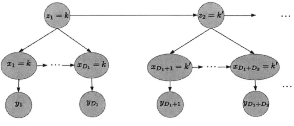
The HSMM has three layers/sequences of random variables. The first layer is a

sequence of "super-states" z,. Each super-state takes a discrete value. The index s is

at a strictly lower frequency than t, and encapsulates a series of time steps {tI,.. , t }

The next layer is the "label" sequence xt. Xt takes on the value of the corresponding

time's super-state. The final layer is the "emission" sequence yt, which is generated by

a state-specific emission probability distribution. It is assumed that the HSMM has

no self-transitions, so that Dt can be interpreted easily. The exhibit below outlines a

Parametric Hidden Semi-Markov Model

K: Number of states (mixture components) {X1, .. ., XT} E K = {1,.. ., K

(1,.. ., T): Sequence of measurements {yi, .. .yT} E Rn

(1,.. ., S): Sequence of "super-states" {z, ... ZS}

C

(1,.. ., S): Sequence of durations {D1, .. .Ds} E R F: Probability distribution governing observation yt

Ok: Parameter governing distribution of observations emitted from kth state

Wk: Parameter governing distribution of dwell time for kth state

irk: Transition probability distribution of state k. 1 1

k = (rkl, ... ,kK)

H(-y): Prior distribution with hyper-parameter of Ok for all k E K

G: Prior distribution of Wk for all k E K

Ok

~ H(')

Dirichlet(A)

(2

2.3

Nonparametric Models

2.3.1

Dirichlet Process

The Dirichlet process (DP) is a distribution over a function space, where the functions are probability measures. The defining characteristic of this family of probability measures, is that each of these probability measures have a countably infinite support. More precisely, a DP, denoted DP(-, H) is a distribution on probability measures on

Figure 2-2: Hidden Semi-Markov Model

a measurable space

E.

E

{

E,

Uk= 8E =

E

E8

E8

for

j

Then, probability measure Go on

E

(Go(e

),

I

-y, H

Dirichlet(yH(e1),

.,

(2.36)

Here E is to be interpreted as a parameter space (i.e., each element 0 E E is a unique parameter). Each element 0 E

E

ek E E which is H-measurable. Observe then that (-H(e1),... ,7 -yH(34)) are a set

of probabilities, weighted by y, where Ek H(Ek) = 1 and H(Ek) ;> 0 for all k. For

every finite partition, H and -y (through this weighted set of probabilities) fixes a

Dirichlet distribution (a probability measure over discrete probability measures with

support being the partition set indexes).

Go can be thought of weighting regions of

E

of fixing different finite partitions of

E.

one fixes set ek E G, and fix different partitions containing O,, it is expected that the average value that Go gives to ek will be H(ek). In fact, E[Go(Ek)

I

A "stick-breaking" construction, devised by Sethuram is a pedagogical description of

the DP which will now be briefly presented. Go is a random probability measure

dis-tributed DP(H, -y). A question that arises is given a sequence of samples {1, ... ,'

where N -+ oo, how does the posterior distribution of Go change. It will turn out that

as the number of samples limits to oo, Go will only have non-zero mass on finitely many

points. The reason is because as more and more samples are produced, the posterior

weighs the base measure less and less (i.e. new parameters stop being spawned), while previously spawned parameters are revisited more frequently. Sethuram proved

that a realization of Go - DP(H, -y) is actually a discrete probability measure with

probability one [221. Let {I&J i be a probability mass function on a countably infinite set where the discrete probabilities are defined as follows:

Dirichlet Process: Stick-breaking Construction

N: Number of measurements {Yi,... YN} E Rn

H(A): Base Measure with hyper parameter A

-y: Concentration parameter

A3 : Weight for kth component; {z1, ... , ZN} E = {1, 2, ...

}

6O: Parameter governing distribution of observations emitted from kth component vk: Auxiliary variable for kth component

Figure 2-3: Dirichlet Process

2.3.2

Hierarchical Dirichlet Process

A Hierarchical Dirichlet process (HDP) is an extension of a Dirichlet process, used to

model groups of data, which are assumed to be generated from a common process,

yet have idiosyncrasies unique to each group. This structure is induced by defining

different group-specific distributions, which will all be generated by a single Dirichlet

6

0,: Unit-mass measure concentrated at 6k

Vk

I

7)

- v

)

(2.38)

H, A

H(A)

(2.39)

Go=

Go is denoted as

#

/

zi

0 -~ #

(2.42)

Yi

I

F(Oz

)

(2.43)

process. Each group-specific distribution Gj (for the jth group).

Gj - DP(a, Go) V j = {1,..., J} (2.45)

All of the groups are tied together by the same Dirichlet process Go.

Go ~ DP(y, H) (2.46)

Given this structure, if one fixes the set A E

e,

every A C

e,

I

The Stick-breaking construction of the HDP is now presented. Let

{y1,

the set of observations for group j. This extends the stick-breaking representation

from the previous section for the hierarchical case. The key fact about an HDP is

that the atoms 0

k are shared not only within groups, but also between groups. Go

establishes an unbounded support of parameters, from which the J groups share their

support. In fact, there exists a non-zero probability the different G share support

points. This is possible because all of the groups are tied to Go. The exhibit below

outlines the Stick-breaking construction of the HDP.

Hierarchical Dirichlet Process: Stick-Breaking Construction

Go(y, H(A)) : Dirichlet process with parameters a, H(A) 1.: Weight for kth component, k E IC = {1, 2, . ..

}

Ok: Parameter governing distribution of observations emitted from kth component

-

|

GEM(-y)

(Go= E

(2.47)

k=1

Ok I H, A ~ H(A) k = 1,2,... (2.48)

J: Number of groups,

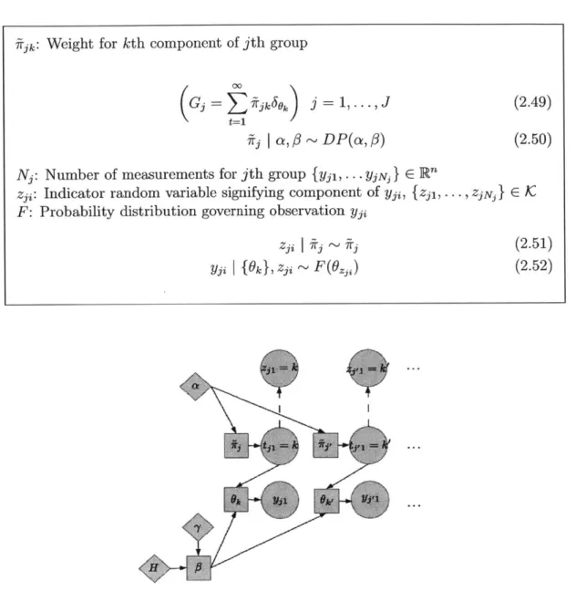
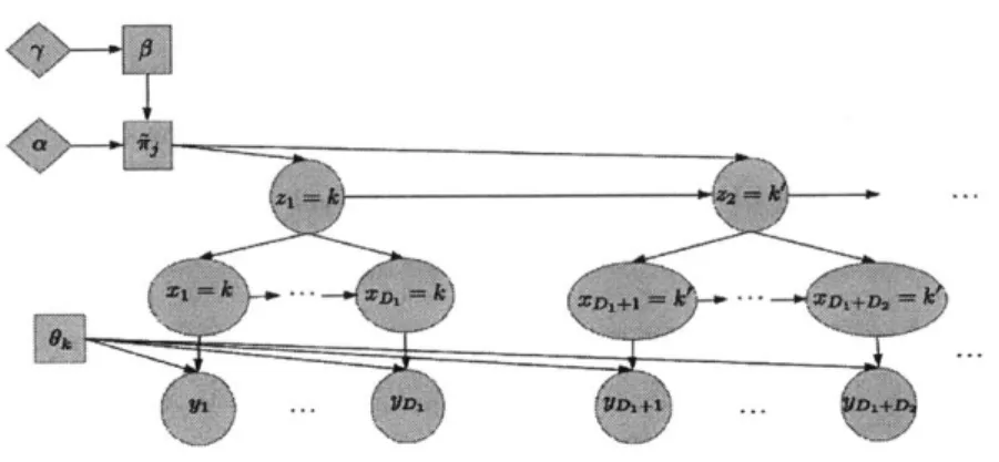
j

Figure 2-4: Hierarchical Dirichlet Process

Teh, et al. metaphorically compares the HDP structure to a "Chinese restaurant

franchise" (CRF) [21]. The CRF is made up of J restaurants, each corresponding to

an HDP group. Within each restaurant is an infinite buffet of dishes corresponding to

parameters {0k}e . This set of dishes is common among all restaurants.

Each customer, corresponding to observation yji is pre-assigned to a given restaurant

determined by that customer's group j. Upon entering the jth restaurant in the CRF,

irjk: Weight for kth component of jth group

G7= Zir.ok) j=1,...,J (2.49)

t=1

-ri I a, / DP(a, /) (2.50)

Nj: Number of measurements for jth group {y, ... yjNj R nR

zji: Indicator random variable signifying component of yji, {zj1, ... , zjNJ} c C

F: Probability distribution governing observation yj

Zyi F(~ ₃ - (2.51)

the customer, corresponding to data point yji (ith customer in the jth restaurant) sits

at one of the currently occupied tables with probability proportional to the number of

people sitting at that table (this distribution is denoted irj) or creates a new table

T+1 (within the jth restaurant) with probability a. The table that customer yji ends

up sitting at is denoted tji.

Whenever a customer is the first customer to sit at a table (implying it is a newly

spawned table), in any of the J restaurants, the customer goes to the buffet line and

chooses from the current set of K dishes, corresponding to {Ok

}Ki1

the franchise or orders a new dish with probability -y (this distribution is denoted

#).

the table tji (denoted by parameter Okjt..) seating yji is known, yji is generated by a

distribution F with parameter 9y

2.3.3

HDP-HMM

Teh, et. al. also presented a formulation of HMMs, extending the HDP (called

"HDP-HMM") as a prior distribution on transition matrices over countably infinite

state spaces [211. In the traditional HDP, explained in the previous section, the data

points yji are pre-partitioned into J groups. Once partitioned, depending on their

group-specific DP Gj, a parameter 0ji, is chosen, deeding on weights Irk, induced by

Gj. The support of parameters is common across all group-specific DPs.

In contrast, the HDP-HMM posits an equivalence between the groups and parameters.

To clarify, assume the previous state zt_1 = k'. k' designates the distribution from

which zt will be chosen, i.e. Zt - irk. Given G0, yt is generated by F(O,,). So, now, the groups are equivalent to the parameters, unlike the traditional HDP. To denote this

significance, we now subscript the parameters 6 with j, instead of k, as done previously.

temporal persistence of states. Fox subsequently introduced an extension: sticky

HDP-HMM, which reduces an HDP-HMM's tendency to rapidly switch between states [191.

This is accomplished by augmenting the HDP-HMM to include a parameter K that

increases the probability of self-transition and a separate prior on this parameter.

Below, we present an exhibit that outlines the HDP-HMM.

HDP-HMM

,3: Dirichlet process with parameters -y, H(A)

Oj: Parameter governing distribution of observations emitted from jth component,

(The group and component index sets are now equal:

J

i~rj: Dirichlet process with parameters a, 3 (state-specific transition distribution

for state j)

(1, . . ., T): Sequence of measurements {yi, ... yT} c Rn

zt: Indicator random variable signifying component of yt, {zi, ... , ZT} E

K

F: Probability distribution governing observation yt

/

I

3)

I

I

K : Self-Transition bias parameter

7r 13|, a, r.-DP a+K) a+ ,i j=1,2,... (2.58)

a+K

2.4

Inference

Bayesian methods for parameter inference are adopted from two perspectives. The first

perspective is based on domain knowledge of the problem. Here, some prior knowledge

parameters, known as a prior. In this setting, bayesian inference is straightforward, since it combines information gathered from data, likelihood to "update" the prior , producing a posterior distribution over the parameters. This posterior distribution is

somehow "better" than the prior, since it takes into account the data points.

There is also the pragmatic perspective. Here, the prior distribution over parameters

is used to make inference tractable. The issue of tractable inference often motivates

the use of conjugate priors. in which the prior and posterior distributions are of

the same form (i.e. in exponential family). Along with tractability, the Bayesian

framework allows for models to flexible, namely hierarchical, with multiple layers. In

this case, priors do not inherently contain information, but their parametric form

will be tailored for tractability. This is why hyper parameters, parameters

govern-ing the distributions of the parameters governgovern-ing the prior are typically inferred, as well.

Bayesian inference, gets its name from Bayes' rule. We see how important conditional

distributions are by examination of this rule. In fact, the likelihood and posterior

distributions are both conditional distributions. Typically, the assumptions a

proba-bilistic model makes in regards to conditional distributions about the random variables

involved, can be easily depicted using graphical models. Graphical models use nodes

to represent random variables and parameters in the probabilistic model and vertices

to depicted probabilistic relations between them. We will also see that the structure

of the conditional dependencies between the random variables and the parameters

of the model is precisely what computational methods such as Gibbs sampling take

advantage of to iteratively compute parameter estimates.

2.4.1

Weak Limit Approximation

In terms of Gibbs sampling the posterior distributions of the Dirichlet process, it is

desirable to maintain a finite approximation to the Dirichlet process mixture model.

One approach to producing such a finite approximation is simply to terminate the

and assign the remaining weight to a single component. This approximation is referred

to as the truncated Dirichlet process.

Let us assume that there are L components in a finite mixture model and we place a finite-dimensional, symmetric Dirichlet prior on these mixture weights:

1 -y - Dir(7/L, . .,y/L) (2.59)

Let G , =

=

f

integrable with respect to the measure H, this finite distribution GL converges weakly

to a countable infinite distribution Go distributed according to a Dirichlet process

[191.

p(zi = k I z\i, 7) = - (2.60)

N -1 +

for each instantiated cluster k. The probability of generating a new cluster is given the remaining mass 7

Another method, motivated by the convergence guarantee of the equation above is to consider the degree L weak limit approximation to the Dirichlet process where L is a number that exceeds the total number of expected mixture components. Both of these approximations, encourage the learning of models with fewer than L components

while allowing the generation of new components, upper bounded by L, as new data are observed [24].

As with the Dirichlet process, the HDP mixture model has an interpretation as the limit of a finite mixture model. Placing a finite Dirichlet prior on 3 induces a finite Dirichlet prior on wrj. As L -+ oo, this model converges in distribution to the HDP mixture model [24]. Inference algorithms for the weak limit approximation of the HDP allows for computational ease and efficiency. Given truncation level L, the weak

limit approximation is as follows,

3 1 -y - Dir(y/L, . ., 7/L) (2.61) (a#,, . . ., a + , . . . , aL) (2.62)

Chapter 3

Non-Bayesian Parametric Model

A non-Bayesian parametric (NBP) HMM (model 1) which will be used to estimate

the degradation rate of a GT rotor, is now presented. In order to model the evolution

of rotor deterioration, a simple model of the the working environment that GenCo's

gas turbines face on any given day must first be established. GenCo supplies bulk

electricity to the wholesale electricity market, creating a stochastic environment with

two main sources of randomness. The first random component is the portion of the

demand of the counter-parties that GenCo must supply. The second component is

the aggregate internal (known only to GenCo) variables-these include company set

thresholds within which the machine must operate, as well as maintenance actions

that the machine must undergo. Even though this last component is endogenous, it is

nonetheless random, as subsystem failure may occur irregularly.

The impact of both of these forces on the rotor must be mathematically defined.

First, notice that these forces affect the evolution of the subsystem at two different

frequencies. The uncertainty in the demand manifests at a much lower frequency due

to the wholesale market structure. This frequency is assumed to be twenty-four hours

(day t) . In contrast, the uncertainty in the endogenous factors operates at a higher frequency. This frequency is set to five minutes (intra-day time r, with 288 total time