HAL Id: hal-02465978
https://hal.inria.fr/hal-02465978
Submitted on 4 Feb 2020
HAL is a multi-disciplinary open access
archive for the deposit and dissemination of
sci-entific research documents, whether they are
pub-lished or not. The documents may come from
teaching and research institutions in France or
abroad, or from public or private research centers.
L’archive ouverte pluridisciplinaire HAL, est
destinée au dépôt et à la diffusion de documents
scientifiques de niveau recherche, publiés ou non,
émanant des établissements d’enseignement et de
recherche français ou étrangers, des laboratoires
publics ou privés.
Curved Path Following of a Farm Tractor Using a
CP-DGPS
Lionel Cordesses, Benoit Thuilot, Philippe Martinet, Christophe Cariou
To cite this version:
Lionel Cordesses, Benoit Thuilot, Philippe Martinet, Christophe Cariou. Curved Path Following of a
Farm Tractor Using a CP-DGPS. SYROCO’00 - 6th IFAC Symposium on Robot Control„ Sep 2000,
Vienne, Austria. pp.489-494, �10.1016/S1474-6670(17)37977-6�. �hal-02465978�
CURVED PATH FOLLOWING OF A FARM TRACTOR USING A CP-DGPS
Lionel Cordesses∗ Benoit Thuilot∗ Philippe Martinet∗ Christophe Cariou∗∗
∗LASMEA - UMR6602 du CNRS, 63177 Aubi`ere, France
∗∗Cemagref, BP 50085, 24 av. des landais 63172 Aubi`ere, France
Abstract: Precision agriculture involves very accurate farm vehicle control along recorded paths. Such repetitive tasks could be handled using Automatic Guided Vehicles (AGV). In this paper, we address the problem of farm tractor control using a single CP-DGPS receiver. A non linear, velocity independent control law has been designed to perform both curved paths and straight lines following. It relies upon the kinematic model of the farm tractor. The control law has been implemented on a commercial farm tractor. Step response as well as curve following are presented and discussed.
Keywords: guidance systems, autonomous mobile robots, robot control, nonlinear control systems, agriculture, implementation.
1. INTRODUCTION
Precision farming can be described as a three steps process. Land surveying is the first one, while agricultural maps recording is the second one. According to the previous steps, the last one could be variable rate seeding, fertilizing,. . . We will focus on the third step, as it requires an accurate vehicle guidance. Let us illustrate this concept in the particular case of a farm tractor. The need for automatic vehicle guidance systems seems obvious on this machine: the driver would only have to finely tune different functions of this machine. Meanwhile, the guidance system would achieve a very accurate positioning, thus insuring neither overlapping nor missing areas.
Many agricultural situations could be reported. Most of them could be classified as two cate-gories. The first one is a ”previously-recorded” path-following task: this trajectory could have
been stored during the seeding for instance, and replayed during weeding. In the second one, the machine must follow a new curve. This curve is computed from the last passage plus an offset (the tool length for instance). We could also mention new possibilities, such as automatic half-turn for driver assistance. All these situations require a control along curved paths.
Many experiments have been conducted and re-ported in the literature. Most approaches can be classified into two categories, as they rely upon two kinds of sensors and information.
1.1 Relative information and guidance systems The first one uses relative information. Re-searchers have focused for instance on the video camera sensor. Mounted at the end of the im-plement or at another appropriate location, it
provides the operator with a set of ”eyes” near the reference line, for instance, a sugar beets row. This contact-free sensing system presents the same off-set information as earlier furrow following or edge-detecting sensors: the reference line to be followed by the vehicle is not the one extracted in the video image. Moreover, it has a challenging feature from a control point of vue: it provides anticipation to the control system, since the camera is scan-ning ahead of the vehicle. Various approaches have been tested. Some rely on 2D information extracted from the image plane (Debain, 1996), (Khadraoui et al., 1998) and (Ollis and Stentz, 1997). Other are based on 3D sensors, for instance made of a laser scanning and a video camera (Chateau et al., 1999). Two kinds of difficulties arise: the first one is the reference extraction. The whole guidance system relies upon the quality and robustness of the image processing algorithms. Extreme conditions of dust, for example, reveal the weakness of the detection side. The other problem arises when the new reference is com-puted in an iterative way from the previous one. The automatic guidance system can lead to oscil-lations. In the same situation, human operators frequently and periodically sacrifice for efficiency. They do not exactly follow the previous path, and often ”straighten out” the edge of the worked area.
1.2 Absolute information and guidance systems The second one uses absolute information. A recent technological development allows accurate three dimensional (3D) positioning of the vehicle in a field without the need for buried cables, field-installed beacons or video sensors: the Global Positioning Systems (GPS). For instance, during the harvest, corn weight measurement devices are coupled to a differential GPS to produce a yield map. It allows farmers to adjust seed, pesticide, and fertilizer to each field location.
State of the art DGPS (Carrier Phase DGPS or CP-DGPS) reach the real-time centimeter accu-racy. This allows the design and implementation of an absolute vehicle guidance system with the availability of a very accurate positioning system. This technology can be used in special operations, in which the vision system is unable to proceed, for instance, in a spraying or fertilizing operation with no visible markers such as boom wheel tracks or foam marks. Researches have been carried out in this area, using fiber optic gyroscopes (FOG) and GPS (Nagasaka et al., 1997). The influence of navigation sensors in GPS based land navigation has also been studied in (Abbot and Powell, 1999). Promising results have been reported where an ” all-GPS ” solution has been preferred: with multiple GPS (O’Connor et al., 1996) or with one GPS (Cordesses et al., 1999).
We will first introduce the reader with the kine-matic model of the farm tractor, with respect to a curved reference. We will then propose a non lin-ear, velocity independent control law designed for curved paths following. A brief description of the straight line case will be derived. Lastly, we will describe our implementation and experimental setup on a farm tractor. Experimental results will be presented and some conclusions will be drawn.
2. VELOCITY INDEPENDENT CONTROL LAW FOR CURVE FOLLOWING In the scope of this paper, we will focus on the particular case of a farm tractor. Most agricul-tural tasks are performed at constant velocity. Unfortunately, this velocity relies upon various factors, such as crop variety and soil properties, and is tuned by the driver. This is the reason why we decided to design a velocity independent control law. Such an approach has been addressed in (Elkaim et al., 1997). We will present here a different solution.
After a brief presentation of the non linear kine-matic model of the farm tractor, we will derive our velocity independent control law for curved path following. We have to mention that we will focus on the path following aspect of the guidance system, while not dealing with the path planning step. In fact, the reference is assumed to exist, as previously stated.
2.1 Kinematic model of the tractor with respect to
a curved reference.
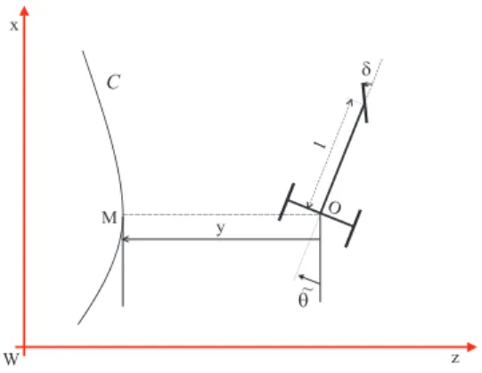
Let (zW x) be an absolute frame. The reference path is assumed to be a curve C in this frame. We will denote s the curvilinear abscissa along C, c(s) the path curvature, and g(s) = dc(s)ds .
The farm tractor model is assumed to match a tricycle model of length l with a controlled front wheel (figure 1). We chose to put the tractor con-trol point at the center of the rear axle, denoted O. Many reasons have led us to use this point. Most of them derive from practical implementation is-sues :
• O is the tractor closest point to the rear
implement. We are highly interested in gath-ering data sensed near the implement, since it performs the agricultural task.
• The GPS antenna antenna must be on the
top of the tractor cabin, to see more satel-lites. Since the control point has to be straight down the antenna, point O suits well. The last reason is a theoretical one. This point
is widely used to deal with the control of car-like systems (Samson, 1995), (Tilbury et al., 1995). Finally, as in (Samson, 1995), we will denote y the distance between O and the closest point M of C. We assume that point O location is always described by a unique couple (s, y). This assump-tion is valid in real world experiments as long as the tractor remains close to the reference path.
Fig. 1. Kinematic model of the farm tractor The configuration of the tractor is thus described without any ambiguity by the state vector X = (s, y, ˜θ)T with :
- s : the curvilinear abscissa of point M - y : the lateral deviation of the tractor with
respect to the reference path.
- ˜θ : the heading of the tractor with respect
to the reference path. It can be described as the angle between the tractor body and the reference tangent at point M .
Two control variables are available, namely U = (v, δ)T with:
- v: linear velocity at point O (the control variable is actually the rotation velocity of the rear wheels, from which the value of v can be inferred).
- δ: orientation of the front wheels (assumed to be superposed, see figure 1).
The vehicle kinematic equations are derived ac-cording to celebrated pure rolling and non-slipping assumptions, and rigid body assump-tions. The former imposes that the linear velocity vector at point O is directed along the vehicle axle. The latter implies that an instantaneous rotation center exists. It has then been proved (see (Samson, 1995)) that the model can write as (for the sake of simplicity, c(s) and g(s) are written hereafter c and g): ˙s = v cos ˜θ 1 − cy ˙y = v sin ˜θ ˙˜θ = v(tan δ l − c cos ˜θ 1 − cy) (1)
The equations are clearly non linear. They become singular when y = 1
c. This means the point O is located at the center of curvature of the reference path. This problem is not encountered in practical situations: the path curvature is small and the farm tractor remains close to the reference.
2.2 Design of a velocity independent control law Farm tractor control along curved paths has al-ready been addressed in some particular cases (Bell et al., 1997). We use hereafter a more general approach: we convert the non linear model (1) into a chained form. Such an approach is interesting as it allows us to use, for a large part, linear systems theory, while still relying upon the non linear model of the plant.
A three dimensional chained form writes as: ˙a1 = m1 ˙a2 = a3m1 ˙a3 = m2 (2) with A = (a1, a2, a3)T and M = (m1, m2)T
respectively the state and control vectors. In order to convert the farm tractor model (1) into chained form (2), let us impose:
a1= s
In order to match (2), the new control m1
neces-sarily writes as:
m1= ˙a∆ 1= v cos ˜θ
1 − cy (3) Moreover, let us impose:
a2= y
We have:
˙a2= v sin ˜θ= a∆ 3m1
Therefore we must choose:
a3= (1 − c y) tan ˜θ
and the last control variable m2is given by:
m2 = ˙a∆ 3 = d
dt((1 − c y)tan˜θ)
= −c v sin ˜θ tan ˜θ − g v cos ˜θ
1 − c ytan˜θ y +(1 − c y)v cos2θ˜ Ã tan δ l − c cos ˜θ 1 − c y ! (4)
In conclusion, the non linear tractor model (1) can be converted into chained form (2) according to the state transformations:
A = Θ(X) with Θ(X) = (s, y, (1 − cy) tan ˜θ)T and the control transformations:
M = Υ(U , X) defined by (3) and (4)
This chained form can be used to design a control law as long as these transformations are invertible,
i.e. v 6= 0 and ˜θ 6= π
2 [π]. From a practical point of
view, once properly initialized, the guided tractor respects these conditions.
In order to get a velocity independent control law, we now replace the time derivative in (2) by a derivation with respect to the curvilinear abscissa
s. The normalized model becomes:
a0 1 = 1 a02 = a3 a03 = m3 with m3= mm21 (5)
The lower part of model (5) is completely linear, so it can be brought to zero using the following virtual control law:
m3= −Kda3− Kpa2 (Kp, Kd) ∈ R+2 (6)
As a matter of fact, reporting (6) in (5), leads to:
a00
2+ Kda02+ Kpa2= 0 (7)
which implies that both a2 and a3, and therefore
y and ˜θ converge to zero.
The above error dynamics is expressed with re-spect to s. So, for any given (Kp, Kd), the re-sulting trajectories remain identical, even if v is varying. This control law is then clearly velocity independent.
Reporting (6) in (3) and (4), the real control is:
δ(y, ˜θ) = arctan à l " cos3θ˜ (1 − c y)2 ³ g y tan ˜θ − Kd(1 − c y) tan ˜θ − Kpy + c (1 − c y) tan2θ˜´+c cos ˜θ 1 − c y #! (8)
The above δ(y, ˜θ) is not bounded, and thus, the
control law does not prevent from actuator satura-tion. It is quite simple to bound the virtual control law m3 to any arbitrary value. Nevertheless, it
leads to a bounded δ only if the trajectory to be followed exhibits some good properties. This is true, for instance, for a circle, where g = 0 and c is constant. The theoretical stability of the closed loop system is still insured, since the chained system is a double integrator (see (Sussmann et
al., 1994)).
2.3 The straight line case
This curved path control law can be gracefully degraded to the case of straight line following. A straight line reference imposes both c = g = 0. The control law (8) then becomes:
δ(y, ˜θ) = arctan(l cos3θ(−K˜
dtan ˜θ − Kpy)) (9)
When we saturate m3using a sigmoid, the
expres-sion of the control law turns to:
δ(y, ˜θ) = arctan
³
K l cos3θ˜1−e−k(Kd tan ˜θ+Kp y)
1+e−k(Kd tan ˜θ+Kp y)
´ (10)
This control law is clearly saturated: K can be tuned so as to ensure: max∀y,∀˜θ|δ(y, ˜θ)| = δmax. Such a control law has been previously designed and used to control a combine harvester along straight lines in a field (Cordesses et al., 1999).
3. EXPERIMENTAL RESULTS
Experiments have been carried out on a farm tractor in our experimental farm in Montoldre, France.
The CP-DGPS dual frequency receiver is a Dassault-Sercel unit: Aquarius 5002 system. Its claimed accuracy is about 1 cm, and its upper sampling frequency is 10 Hz. Three dimensional velocities are computed thanks to Doppler mea-surements. Its short initialization time allows its use in many farm applications.
The controller has been implemented in high level language (C++) on a Pentium based computer.
3.1 Implementation of a state measurement unit Both control laws (8) and (9) require lateral deviation y and heading error ˜θ.
Since the GPS antenna is straight up the point O, the receiver only provides us with the 3D position and velocity of that point.
The y measurement is easily obtained from the knowledge of the reference path and the O coordi-nates. The ˜θ is more complex to derive. A common
and costly solution makes use of additional hard-ware and sensor (either a gyroscope or an attitude measurement unit). We have preferred a cheaper approach based upon our only exteroceptive sen-sor, the CP-DGPS receiver. Under the previously mentioned pure rolling and non-slipping assump-tions, one can easily infer the heading of the farm tractor thanks to realtime velocity data.
3.2 Step response of the system
Although a step path is not common in agricul-ture, we have used the step response to check the behaviour of our closed loop system. All the experiments have been conducted on an almost flat ground with the straight line control law (10). The very first experiments have been carried out with a 2 meters step at 8 km/h. One can compare on figure 2 simulation and experimental results.
0 50 100 150 −0.5 0 0.5 1 1.5 2 2.5
Simulated and experimental step response of the farm tractor (8 km/h)
z (meter)
x (meter) Reference path
Lateral deviation Simulation result
Fig. 2. Simulation and experimental trajectory at 8 km/h
We have also checked the velocity independence property. Experiments have been conducted at 4 and 8 km/h (constant velocity) and from 4 to 8 km/h (varying velocity). One can check on the upper curve of figure 3 that the three step responses almost perfectly overlap. The lower curve plots the raw velocity as computed by the GPS receiver. One can notice the sound behaviour of the farm tractor during all these experiments.
30 40 50 60 70 80 90 100 110 120 0 0.5 1 1.5 2
Farm tractor trajectory at 4 km/h, 8 km/h and 4 to 8 km/h
z (m) x (m) 30 40 50 60 70 80 90 100 110 120 2 4 6 8 10 12 z (m) velocity (km/h)
Farm tractor velocity
Fig. 3. Velocity independence validation
Standard deviation from the mean σx, and bias
µx of the lateral deviation for these experiments are summed up in table I. One can notice that the results appear quite satisfactory (σx< 3.1 cm
and µx< 2.7 cm).
Table I. Bias and standard deviation from mean velocity (km.h−1) 4 8 4 to 8
µx (cm) 2.7 0.3 2.1
σx(cm) 1.9 3.1 3.1
3.3 Curve following
Up to now, we have only validated the straight line following law. In the sequel of these experiments, we now investigate the curved path following control law (8).
We first recorded in open loop a reference path, roughly made of straight lines and a quarter of circle (figure 4).
The closed loop experiments with respect to this new path started with a 0.8 m lateral deviation (see figure 5 at initial time). One can notice that the farm vehicle has converged to the reference path (both curves overlap on figure 5). The bias is about 3 cm and the standard deviation from the mean less than 5 cm. Moreover, the maximum lateral deviation along the whole path is 18.4 cm (see figure 5 at time t = 30 s). The curvature of the reference path at this time is the highest one, thus leading to a δ varying very quickly.
0 20 40 60 80 100 120 140 −80 −70 −60 −50 −40 −30 −20 −10 0 10
Farm tractor trajectory
z (m)
x (m)
Fig. 4. Reference path and closed loop, farm tractor trajectory 1.5 2 2.5 3 3.5 −18 −17.5 −17 −16.5
Zoomed trajectory − worst case
z (m) x (m) 0 10 20 30 40 50 60 70 80 90 100 −0.8 −0.7 −0.6 −0.5 −0.4 −0.3 −0.2 −0.1 0 0.1 0.2
Lateral deviation with respect to a curved reference
Time (s)
y (m)
highest curvature
Fig. 5. Lateral deviation with respect to the curved reference
Such a behaviour can be explained. Our investi-gations have led us to incriminate the low level servoing system. First of all, one must keep in mind this system does have a response time (a few hundreds of milliseconds). Moreover, it has not been optimized for fast tracking: neither the hydraulic components nor the controller - off the shelves devices - can achieve very high perfor-mances.
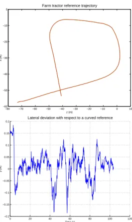
We have recorded a second reference path: it is longer than the previous one, and crosses different types of ground (figure 6). Thorough analysis of the lateral deviation leads to the same conclu-sions.
−80 −70 −60 −50 −40 −30 −20 −10 0 10 −60 −50 −40 −30 −20 −10 0
Farm tractor reference trajectory
z (m) x (m) 0 20 40 60 80 100 120 −0.2 −0.15 −0.1 −0.05 0 0.05 0.1 0.15 0.2
Lateral deviation with respect to a curved reference
Time (s)
y (m)
Fig. 6. Second reference path 4. CONCLUSION
The purpose of this work was to control a farm tractor along a curved path, using a CP-DGPS sensor.
We first built a non linear control law using a chained form of the kinematic model of the farm tractor. Moreover, it has been designed so as to be velocity independent for practical reasons. We have implemented this control law on a farm tractor. Curved path following has been demon-strated. We have also checked the velocity inde-pendence property.
Although results are quite satisfying on an almost flat ground, further research has to be done to take into account for slope. One can also mention the use of other sensors to insure a highest level of reliability, and thus security.
Another important issue is to build a better hydraulic servoing system, in order to decrease both latency time and response time. One could also take into account for the latency of the whole vehicle thanks to an anticipatory system.
REFERENCES
Abbot, A. and D. Powell (1999). Land - vehicle navigation using GPS. Proceedings of IEEE 87(1), 145–162.
Bell, T., M. O’Connor, V. K. Jones, A. Rekow, G. Elkaim and B. Parkinson (1997). Realistic autofarming closed-loop tractor control over irregular paths using kinematic GPS. In:
Eu-ropean Conf. on Precision Agriculture. Vol. 1.
Chateau, T., F. Collange, L. Trassoudaine, C. De-bain and J. Alizon (1999). Fusion d’attributs: application au guidage d’engins agricoles. In: LFA’99 Rencontres francophones sur la
logique floue et ses applications. pp. 141–148.
Cordesses, L., P. Martinet, B. Thuilot and M. Berducat (1999). GPS-based control of a land vehicle. In: IAARC/IFAC/IEEE Intern.
Symp. on Automation and Robotics in Con-struction (ISARC’99). Vol. 1. pp. 41–46.
Debain, C. (1996). Lois de commande pour le contrˆole et la mobilit´e de machines agri-coles. PhD thesis. Universit´e Blaise-Pascal. Clermont-Ferrand, France.
Elkaim, G., M. O’Connor, T. Bell and B. Parkin-son (1997). System identification and robust control of farm vehicles using CDGPS. In:
Proceedings of the 10th International
Meet-ing of the Satellite Division of the Insitute of Navigation. Vol. 2. ION-GPS-97. Kansas
City, Missouri, USA. pp. 1415–1424.
Khadraoui, D., C. Debain, R. Rouveure, P. Mar-tinet, P. Bonton and J. Gallice (1998). Vi-sion based control in driving assistance of agricultural vehicles. International Journal of
Robotics Research 17(10), 1040–1054.
Nagasaka, Y., R. Otani, K. Shigeta and K. Tani-waki (1997). Automated operation in paddy fields with a fiber optic gyro sensor and GPS. In: Proceedings of the Intern. Workshop on
Robotics and Automated Machinery for Bio-Productions, BIO-ROBOTICS’97. pp. 21–26.
O’Connor, M., G. Elkaim, T. Bell and B. Parkin-son (1996). Automatic steering of a farm ve-hicle using GPS. In: Proceedings of the
Inter-national Conference on Precision Agriculture 1996. Vol. 3. pp. 767–777.
Ollis, M. and A. Stentz (1997). Vision based per-ception for an automated harvester. In:
Pro-ceedings of the IEEE Intern. Conf. on Intel-ligent Robots and Systems. Vol. 2. IROS’97.
Grenoble, France. pp. 1838–1844.
Samson, C. (1995). Control of chained sys-tems. Application to path following and time-varying point stabilization of mobile robots. IEEE Trans. on Automatic Control 40(1), 64–77.
Sussmann, H., E. Sontag and Y. Yang (1994). A general result on the stabilization of linear systems using bounded controls. IEEE Trans.
on Automatic Control 39(12), 2411–2425.
Tilbury, D., O. J. Sordalen, L. Bushnell and S.S. Sastry (1995). A multisteering trailer system: conversion into chained form using
dynamic feedback. IEEE Trans. on Robotics