HAL Id: tel-01496107
https://tel.archives-ouvertes.fr/tel-01496107
Submitted on 27 Mar 2017
HAL is a multi-disciplinary open access archive for the deposit and dissemination of sci-entific research documents, whether they are pub-lished or not. The documents may come from teaching and research institutions in France or abroad, or from public or private research centers.
L’archive ouverte pluridisciplinaire HAL, est destinée au dépôt et à la diffusion de documents scientifiques de niveau recherche, publiés ou non, émanant des établissements d’enseignement et de recherche français ou étrangers, des laboratoires publics ou privés.
Characterization of planetary subsurfaces with
permittivity probes : analysis of the
SESAME-PP/Philae and PWA-MIP/HASI/Huygens
data
Anthony Lethuillier
To cite this version:
Anthony Lethuillier. Characterization of planetary subsurfaces with permittivity probes : analysis of the SESAME-PP/Philae and PWA-MIP/HASI/Huygens data. Astrophysics [astro-ph]. Université Paris Saclay (COmUE), 2016. English. �NNT : 2016SACLV071�. �tel-01496107�
1
NNT : 2016SACLV071
T
HESE DE DOCTORAT
DE
L’U
NIVERSITE
P
ARIS
-S
ACLAY
PREPAREE A
L’U
NIVERSITE DE
V
ERSAILLES
ST-Q
UENTIN
-E
N
-Y
VELINES
ECOLE DOCTORALE N° (127)
Astronomie et astrophysique d'Ile-de-France
Sciences de l'Univers
Par
Mr Lethuillier Anthony
Characterization of planetary subsurfaces with permittivity probes: analysis of the
SESAME-PP/Philae and PWA-MIP/HASI/Huygens data.
Thèse présentée et soutenue à Guyancourt, le 21 septembre 2016 :
Composition du Jury :
Mme, Carrasco Nathalie Professeure / UVSQ Présidente du Jury
Mme, Pettinelli Elena Professeure / Université de Rome 3 Rapporteur
M, Quirico Eric Professeur / Université Joseph Fourier Grenoble Rapporteur
M, Lasue Jérémie Astronome-Adjoint / Université de Toulouse Examinateur M, Lebreton Jean-Pierre Chargée de Recherche / LPC2E Examinateur
Mme, Ciarletti Valérie Professeure / UVSQ Directeur de thèse
Mme, Le Gall Alice Maître de Conférences / UVSQ Co-directeur de thèse
2
Titre : Caractérisation des subsurfaces planétaires à l’aide de sondes de permittivité : analyse des données
SESAME-PP/Philae/Rosetta et PWA-MIP/HASI/Huygens/Cassini-Huygens.
Mots clés : Rosetta/Philae, Cassini/Huygens, comètes, Titan, sous-surface, permittivité
Résumé : Les sondes de permittivité sont des instruments de prospection géophysique non destructifs qui
donnent accès aux propriétés électriques, aux basses fréquences (10 Hz-10 kHz), de la proche subsurface. Ce faisant, elles renseignent sur la composition, porosité, température et éventuelle hétérogénéité des premiers mètres sous la surface.
Utilisant généralement 4 électrodes, le principe des sondes de permittivité est simple : il consiste à injecter un courant sinusoïdal de phase et d’amplitude connues entre deux électrodes (dipôle émetteur) et à mesurer l'impédance mutuelle (le rapport complexe entre la tension et le courant injecté) entre ce dipôle émetteur et un dipôle récepteur. La permittivité complexe du matériau de surface, à savoir sa constante diélectrique et sa conductivité électrique, sont alors déduites de la mesure de l’amplitude et de la phase de cette impédance mutuelle. Les fréquences d’opération des sondes de permittivités sont basses là où l’approximation quasi-statique s’applique. A ce jour, les propriétés électriques de seulement deux surfaces planétaires extraterrestres ont été étudiées par des sondes de permittivité : celle de Titan par l’instrument PWA-MIP/HASI/Huygens/Cassini-Huygens et celle du noyau de la comète 67P/Churyumov–Gerasimenko par SESAME-PP/Philae/Rosetta.
Nous présentons la première analyse des données obtenues par SESAME-PP à la surface de la comète 67P/Churyumov–Gerasimenko. Grâce à un travail précis (1) de modélisation numérique de l’instrument et de son fonctionnement, (2) de campagne de mesures (en laboratoire et dans des grottes de glace) afin de valider la méthode d’analyse et (3) d’hypothèses réalistes sur l’environnement proche de la sonde, nous avons pu contraindre la composition et surtout la porosité des premiers mètres du noyau cométaire montrant qu’ils étaient plus compacts que son intérieur. Nous avons également travaillé à une nouvelle analyse des données obtenues en 2005 par PWA-MIP proposant notamment de nouveaux scénarios pour le changement brutal de propriétés électriques observé 11 min après l’atterrissage de Huygens. Ces nouveaux scénarios s’appuient, entre autres, sur les mesures de caractérisation électrique menées au LATMOS sur des échantillons de composés organiques (tholins), analogues possibles des matériaux recouvrant la surface de Titan.
Title: Characterization of planetary subsurfaces with permittivity probes: analysis of the SESAME-PP/Philae
and PWA-MIP/HASI/Huygens data.
Keywords: Rosetta/Philae, Cassini/Huygens, Comets, Titan, subsurface, permittivity
Abstract: Permittivity probes are non-destructive geophysical prospecting instruments that give access to the
low frequency (10 Hz – 10 kHz) electrical properties of the close subsurface. This provides us with information on the composition, porosity, temperature, and heterogeneity of the first meters of the subsurface.
Using 4 electrodes, the technique consists in injecting a sinusoidal current of known phase and amplitude between two electrodes (transmitting dipole) and measuring the mutual impedance (complex ratio of measured potential over injected current) between this dipole and a receiving dipole. The complex permittivity (i.e. dielectric constant and conductivity) of the subsurface material is derived from the measured phase and amplitude of the mutual impedance. The frequency range of operation of permittivity probes is low, therefore the quasi static approximation applies. To this day the electrical properties of only two extra-terrestrial surfaces have been studied by permittivity probes, the surface of Titan by the instrument PWA-MIP/HASI/Huygens/Cassini-Huygens and the surface of the nucleus of comet 67P/Churyumov–Gerasimenko by SESAME-PP/Philae/Rosetta.
We present a first analysis of the data collected by SESAME-PP at the surface of the comet 67P/Churyumov–Gerasimenko. With the help of (1) precise numerical models of the instrument, (2) field measurements (in a controlled and natural environment) in order to validate the analysis method, and (3) realistic hypothesis on the close environment we were able to constrain the composition and porosity of the first meters of the comet’s nucleus, showing that the subsurface is more compact than its interior. We also reanalysed of the data collected in 2005 by PWA-MIP, offering new explanations for the abrupt change in the electrical properties observed 11 minutes after the landing of Huygens. These new scenarios were built in the light of lab measurements performed at LATMOS on samples of organic matter (tholins), possible analogue of Titan’s surface material.
3
“In the beginning the Universe was created. This has made a lot of people very angry and
been widely regarded as a bad move.”
Douglas Adams
“You need to read more science fiction. Nobody who reads science fiction comes out with
this crap about the end of history”
Iain M Banks
4
Acknowledgments
During my three years at LATMOS I have had the opportunity to work, interact, and exchange with many people all around the world, without their help and support this work would not be what it is today.
First and foremost, I would like to thank my two advisors, Alice Le Gall and Valerie Ciarletti who gave me the opportunity to pursue this work and helped me (with a lot of patience) to get through it. It was an honor and a pleasure working under their supervision and they taught me many invaluable lessons which will serve me greatly in the future.
I would like to also thank the people who reviewed my manuscript, Elena Pettinelli and Eric Quirico and those that examined it, Nathalie Carrasco, Jean-Pierre Lebreton and Jérémie Lasue. They helped make this work shine to the fullest.
At LATMOS I was helped immensely by Michel Hamelin and Sylvain Caujolle-Bert who assisted me in many parts of my research. They also had the ungrateful job of explaining electronics to a geologist.
I am grateful to all the members of the SESAME-PP team, Rejean Grard, Walter Schmidt, Klaus J. Seidensticker, Hans-Herbert Fischer and Roland Trautner, and to the Rosetta team in general without whom the SESAME-PP/Philae/Rosetta instrument would not have been possible.
Thanks also to everybody at LATMOS (IT, administration staff, service personnel, engineers and scientists) for making the lab a great work environment, I want to thank the IMPEC team in particular, with whom it was always a pleasure to exchange ideas about our research and who provided many pertinent criticisms that helped me improve as a scientist (especially through the young scientist meetings).
The measurement on tholins would not have been possible without the help of Williams Brett, Francis Schreiber and the ATMOSIM team who provided us with the samples studied.
Finally, but by no means least, a big thanks to all my friends who were always there for me, thank you to my family who always pushed me and helped me get through my studies and gave me the freedom of studying what I loved. A most loving thanks to my wife Alexia for her unbelievable support, proofreading, and cooking; I am infinitely grateful to her for having the patience of dealing with a perpetually distracted husband.
5
Acronyms
67/C-G 67P/Churyumov–Gerasimenko
ADC Analog-to-Digital-Converter
APXS Alpha-P-X-ray Spectrometer
CASSE Comet Acoustic Surface Sounding Experiment
CIMM Capacitance-Influence Matrix Method
CIVA Comet Infrared and Visible Analyzer
CONSERT Comet Nucleus Sounding Experiment by Radio wave Transmission
COSAC COmetary SAmpling and Composition
COSIMA Cometary Secondary Ion Mass Analyzer
DAC Digital-to-Analog-Converter
DIM Dust Impact Monitor
EGSE Electrical Ground Support Equipment
ELF Extremely Low Frequency
ESA European Space Agency
FMI Finnish Meteorological Institute
FPGA Field-Programmable Gate Array
FSS First Science Sequence
GIADA Grain Impact Analyser and Dust Accumulator
HASI Huygens Atmospheric Structure Instrument
HF High Frequency
LATMOS Laboratoire Atmosphères, Milieux, Observations Spatiales
LTS Long Term Science
MARSIS Mars Advanced Radar for Subsurface and Ionosphere Sounding
MIDAS Micro-Imaging Dust Analysis System
MIP Mutual Impedance Probe
MUPUS MUlti PUrpose Sensor for Surface and Subsurface Science
MIRO Microwave Instrument for the Rosetta Orbiter
NASA National Aeronautics and Space Administration
OSIRIS Optical, Spectroscopic and Infrared Remote Imaging System
6
PWA-MIP Permittivity, Waves and Altimetry-MIP
Radars RAdio Detection And Ranging
ROLIS ROsetta Lander Imaging System
ROMAP ROsetta lander Magnetometer And Plasma monitor
ROSINA Rosetta Orbiter Spectrometer for Ion and Neutral Analysis
RPC Rosetta Plasma Consortium
RSI Radio Science Investigation
RSSD Research and Scientific Support Department
SD2 Sample Drilling and Distribution
SDL Separation Descent and Landing
SESAME Surface Electrical, Seismic and Acoustic Monitoring Experiments
SHARAD SHAllow RADar
TDEM Time Domain Electromagnetic Method
UHF Ultra High Frequency
VES Vertical Electrical Sounding
VIRTIS Visible and Infrared Mapping Spectrometer
VLF Very Low Frequency
Notations
𝐸⃗ electric field
𝐵⃗ magnetic field
𝑡 time
𝐷⃗⃗ electric displacement field
𝐻⃗⃗ magnetizing field
𝐽 𝑇 total current density
𝐽 𝑐 current density
𝐽 𝐷 displacement current
𝜌̅ the charge density
𝑃⃗ polarization field
𝜀0 permittivity of free space
7
𝑀⃗⃗ the magnetization field
𝜒 electrical susceptibility
𝜖 permittivity
𝜎 conductivity
𝜌 resistivity
𝜖𝑒𝑓𝑓 effective permittivity
𝜎𝑒𝑓𝑓 effective electric conductivity
𝜖𝑟 complex relative permittivity
𝜖𝑟′ dielectric constant
𝜖𝑟′′ imaginary part of the complex relative permittivity
𝜔 rotational frequency
tan 𝛿 loss tangent
𝜖𝑟𝑠 static permittivity
𝜖𝑟∞ relative high-frequency limit permittivity
𝜏 relaxation time 𝑇 temperature 𝑘𝐵 Boltzmann constant 𝐸 activation energy 𝑉 electric potential Δ𝑉 potential difference
𝐴 period of atomic vibrations
𝑅, 𝑟 distances
𝐼 current
𝑄, 𝑞 electric charge
𝛿𝑠, 𝛿 geometrical factor of an array
𝑍𝑚 mutual impedance
𝑍0 mutual impedance in vacuum
𝑅𝑒 real part
𝐼𝑚 imaginary part
𝛿𝑠𝑑 electrical skin depth
𝜆 wavelength
8
𝑐 velocity of light in vacuum
𝐾𝑘𝑛𝑚 coefficients of the medium capacitance-influence matrix
[𝑲] capacitance-influence matrix of the multi-conductor system [𝑲𝒆] electronic matrix
[𝑲𝒎] environnement capacitance-influence matrix
𝐶 capacitance
9
Index
Acronyms ... 1 Notations ... 6 Index... 9 Introduction ... 14Chapter 1: Characterizing subsurface electric properties ... 17
1. Interaction of electromagnetic fields with matter ... 17
1.1. Maxwell’s equations ... 17
1.2. Frequency dependence of the relative permittivity ... 21
1.3. Propagation and diffusion domains ... 23
2. Electrical properties of natural matter ... 23
2.1. Water ice ... 23 2.2. Liquid water ... 25 2.3. Rocks ... 27 2.4. Chondrites... 28 2.5. Lunar regolith ... 30 2.6. Martian analogs ... 30
2.7. Europa crust analog ... 31
3. Mixing laws ... 32
4. Methods for the characterization of subsurface electric properties ... 36
4.1. Vertical Electrical Sounding (VES) ... 36
4.2. Time Domain Electromagnetic Method (TDEM) ... 38
4.3. Self-impedance probes ... 39
4.4. Mutual impedance probes (MIP) ... 41
4.5. Radars ... 43 4.5.1. Radars in reflection ... 43 4.5.2. Radars in transmission ... 45 4.6. Microwave radiometers... 46 4.7. Comparing techniques ... 47 5. Concluding remarks ... 48
10
1. History and theory of surface Mutual Impedance Probes (MIP) ... 50
1.1. History of MIP ... 50
1.2. Mutual impedance for a quadrupole above a surface: derivation of the surface complex permittivity ... 51
2. Numerical modelling and Capacity-Influence Matrix method ... 54
2.1. Application to realistic problems ... 54
2.2. Derived complex permittivity ... 54
2.3. Comparing simple examples to more realistic cases ... 55
2.3.1. Finite size electrodes ... 55
2.3.2. Presence of conducting elements close to the electrodes ... 56
2.3.3. Influence of the electronics circuit ... 58
2.4. The Capacitance-Influence Matrix Method (CIMM) ... 58
2.5. Derivation of 𝝐𝒓 ... 60
3. Validation of the use of numerical models ... 61
3.1. Method of image charges ... 62
3.1. Simplified model of a MIP ... 64
3.2. Comparison ... 65
4. Exploring the capabilities of the mutual impedance probes ... 66
4.1. Sensitivity of the transmitting electrodes ... 67
4.2. Sounding depth ... 68
4.3. Heterogeneous subsurfaces ... 70
4.3.1. Study cases ... 70
4.3.2. Derived permittivity ... 72
4.4. Maximizing the scientific output ... 73
5. Concluding remarks ... 74
Chapter 3: The SESAME-PP/Philae/Rosetta experiment: modelling approaches and performances ... 75
1. The SESAME-PP/Philae/Rosetta experiment ... 75
1.1. Comets and Rosetta’s mission objectives ... 76
1.1.1. Comets and their scientific interests ... 76
1.1.2. Scientific objectives and description of the Rosetta mission ... 78
1.2. Rosetta’s and Philae’s payload ... 78
1.2.1. Rosetta’s payload ... 78
1.2.2. Philae’s payload ... 81
1.2.3. Depth sounded ... 83
1.3. The SESAME-PP experiment ... 84
11
1.3.2. The SESAME-PP experiment and operation modes ... 85
2. Modeling SESAME-PP ... 91
2.1. SESAME-PP numerical model ... 91
2.2. SESAME-PP lumped element model ... 92
2.3. Application of the Capacity-Influence Matrix Method ... 95
Step 1: Derivation of medium capacitance-influence matrix 𝐾𝑚 ... 95
Step 2: Derivation of the electronic matrix 𝐾𝑒... 96
Step 3: Solving the numerical model ... 98
2.4. SESAME-PP laboratory model ... 99
2.4.1. Description of the laboratory replica of SESAME-PP ... 99
2.4.2. Description of the Lander replica ... 101
2.5. Experimental tests in a controlled environment and validation of the numerical model ... 102
2.5.1. General considerations ... 102
2.5.2. Three-foot configuration measurements in a controlled environment ... 102
2.5.3. Five-electrode configuration in a controlled environment ... 110
2.6. Tests in a natural environment and comparison with the numerical model... 113
2.6.1. Dachstein field campaign ... 114
2.6.2. Description of the area studied ... 114
2.6.3. Three-foot configuration measurements over an icy surface... 115
2.7. Sounding depth of SESAME-PP ... 118
3. Concluding remarks ... 119
Chapter 4: Electrical properties and porosity of the first meter of 67P/Churyumov-Gerasimenko’s nucleus as constrained by SESAME-PP/Philae/Rosetta ... 121
1. RDV, landing and escort ... 122
1.1. The cruise phase and Rosetta “rendez-vous “with 67P/C-G ... 122
1.2. Philae separation and landing at Abydos... 124
1.3. Escort phase ... 127
2. Main results from the Rosetta mission ... 127
2.1. Nucleus ... 127
2.2. Coma ... 133
2.3. Context of the SESAME-PP measurements... 135
3. SESAME-PP observations during the cruise, descent and landing ... 135
3.1. Cruise ... 135
3.2. Separation, Descent, Landing (SDL) ... 138
12
4. Analysis of the SESAME-PP surface data ... 143
4.1. Approach... 143
4.2. FSS passive measurements ... 143
4.3. Transmitted currents ... 144
4.4. Received potentials... 145
4.4.1. Reconstruction of Philae attitude and environment at Abydos ... 146
4.4.2. Retrieval of the dielectric constant of the near surface of Abydos ... 148
5. Implications for the composition and porosity of the first meter of 67P/C-G’s nucleus ... 149
6. Concluding remarks ... 153
Chapter 5: The PWA-MIP/HASI/Huygens instrument, revisiting the data collected on the surface of Titan 154 1. The Cassini/Huygens mission and Titan ... 155
1.1. The Cassini/Huygens mission in brief ... 155
1.2. Titan after Cassini-Huygens ... 155
2. The PWA-MIP/HASI instrument ... 158
2.1. Description ... 158
2.1.1. Transmitting circuit ... 159
2.1.2. Receiving circuit ... 160
2.2. Numerical geometry model ... 160
2.3. Electronic model ... 161
2.4. Sounding depth ... 162
3. Data collected during descent and on the surface ... 163
3.1. Descent measurements ... 164
3.2. Surface measurements ... 164
4. Data calibration and analysis ... 165
4.1. Data calibration and electronic matrix ... 165
4.2. PWA-MIP/HASI configuration of operation at the Huygens landing site ... 166
4.3. Derived permittivity ... 169
4.4. Titan’s first meter surface composition ... 172
4.5. The 9539 s event ... 174
5. Electrical properties of analogues of Titan’s organic materials ... 175
5.1. Tholins ... 175
5.2. Description of the measurement bench ... 178
5.3. Measurement and derivation of the sample complex permittivity ... 179
13
6.1. Frequency and temperature dependence ... 182
6.2. Porosity dependence ... 184
6.3. Derivation of the complex permittivity of bulk tholins ... 185
7. Constrains on Titan’s subsurface composition ... 187
6.2 The liquid inclusion model ... 188
7.1. Thin conductive surface layer model ... 190
8. Concluding remarks ... 193
Conclusion ... 195
14
Introduction
The subsurfaces of planetary objects, i.e. the interface between their deep interior and an atmosphere or a vacuum, are the hosts of exogenic (weathering, thermal stress, impacts, radiations…) and/or endogenic (volcanism, tectonism, …) processes whose signatures may still be measurable. The exploration of planetary subsurfaces has the potential of unveiling these processes and thus the story of the formation and evolution of celestial objects.
Among the techniques developed to study planetary subsurfaces, electromagnetic sounding methods have the advantage of being non-destructive. The first recorded use of such a method dates back to the beginning of the 20th century when Wenner published an article entitled “A method for
measuring earth resistivity” in the Bulletin of the Bureau of Standards. Since then, other techniques have been proposed, RADAR being one of the most used, and rapidly found applications in research as well as in industry. However, in space and planetary exploration, the use of electromagnetic method is relatively recent. Earth-based radars were used in the fifties for the observation of the Moon and meteors but the first sounding experiments (Surface Electrical Properties experiment & ASLE) to fly on board a spacecraft was conducted in the frame of the Apollo 17 lunar mission (1967) and the first planetary radar sounder (MARSIS/Mars Express) was sent to Mars in 2004.
Mutual Impedance Probes (MIP), also called Permittivity Probes (PP), are one of these electromagnetic sounding methods. They are commonly used on Earth, in agronomical and archaeological surveys, to map the electrical properties of soils. MIP measure the complex permittivity, i.e. the dielectric polarizability (or dielectric constant) and electrical conductivity, within the first meters below the surface. These parameters depend on composition and physical state (porosity, heterogeneity…) of the subsurface. Monitoring the variation of the permittivity as a function of space (geological structure), time (day, season) and other environmental properties (temperature) thus provides key insights on the subsurface that can be correlated with the data collected by other means.
Mutual Impedance Probes are based on the quadrupole array technique. The principle of the measurement is as follows. The instrument uses 4 electrodes, generally (but not necessarily) in contact with the ground. In the active mode, a sinusoidal current of frequency generally between 10 Hz and 10 kHz, and known phase and amplitude is injected between two electrodes (transmitting monopole), and the voltage induced between two other electrodes (receiving dipole) is measured. The inferred transfer, or Mutual Impedance (MI) of the array in the quasi-static approximation, i.e. the complex ratio of measured voltage upon injected current, gives access to the complex permittivity of the
15
subsurface at a given frequency that can be varied in the ELF-VLF (Extremely Low Frequency-Very Low Frequency) range. Of importance, at frequencies below 10 kHz, the electrical signature of a material is especially sensitive to the presence of water ice and to its temperature; MIP are thus well suited to the soundings of icy objects such as comets.
To date, two MIPs have flown on space missions. The complex permittivity at low frequency of an extraterrestrial surface was investigated in situ for the first time by PWA-MIP/HASI (Permittivity, Waves and Altimetry-MIP/Huygens Atmospheric Structure Instrument) carried by the ESA Huygens Probe that landed on the surface of Titan, the largest moon of Saturn, on 14 January 2005 in the frame of the Cassini-Huygens mission (NASA/ESA/ASI). Almost ten years later, on November 13, 2014, the SESAME-PP/Philae (Surface Electrical, Seismic and Acoustic Monitoring Experiments - Permittivity Probe) performed measurements on the surface of the nucleus of comet 67P/Churyumov-Gerasimenko in the frame of the Rosetta mission (ESA). The present work is dedicated to the analysis of the data collected by SESAME-PP at the final landing site (called Abydos) of the Philae module as well as to the re-assement of the derivation of the complex permittivity of Titan’s surface with PWA-MIP/HASI. Titan and comets being of great interest for the understanding of the origin of the Solar System and of life on Earth as well as for the search of potential extraterrestrial life, this work is a contribution to key scientific questions.
The present manuscript is composed of five chapters. The first chapter presents the theoretical background of electromagnetic wave interaction with matter as well as a non-exhaustive review of electrical properties of materials relevant to planetary subsurfaces and of the main electromagnetic sounding methods. The second chapter is dedicated to the description of MIP and the approach that we have developed to analyze their data. If the principle of a MIP is simple in theory, in practice, the conductive environment of the instrument (e.g., due to the vicinity of a lander body), the configuration of operation and the electronic circuit have a strong influence on the measurements and thus on the retrieval of the subsurface electrical properties. To address this issue, a numerical approach, based on the Capacitance-Influence Matrix Method (CIMM), has been proposed. In Chapter 2, we present and validate this approach in order to assess the general performances of MIP (sounding depth, heterogeneous subsurface characterization). In Chapter 3, we present the numerical models especially developed for the analysis of SESAME-PP data and validated them by comparison with measurements performed with a laboratory replica of the SESAME-PP instrument, both in a controlled environment (over a perfect electrical reflector) and over a natural icy surface (in the Austrian caves of Dachstein). Chapter 4 describes the data collected by SESAME-PP at Philae final landing site and their analysis. We emphasize that the analysis approach that we have developed takes into account the attitude of the instrument in its environment, which, in the case of Philae at Abydos, was far from
16 nominal. We reconstituted the attitude and environment of Philae using all available constraints from other Rosetta instruments. The results of SESAME-PP data analysis and their implications are discussed in the light of other (Rosetta and non-Rosetta) instrument findings. Lastly, we present in Chapter 5 the re-assement of the data collected at the surface of Titan by PWA-MIP/HASI, accounting for new insights on the final resting position of the Huygens capsule. We also propose scenarios to explain the sudden change of the subsurface electrical properties detected about 11 min after Huygens landing. In support of this analysis, laboratory measurements were performed at LATMOS to characterize the electrical properties of tholins, potential analogs of the complex organic molecules formed by photolysis in the atmosphere of Titan. These measurements are presented and used to constrain the composition of the first meters of Titan using PWA-MIP/HASI result.
This work was performed at the LATMOS (Laboratoire Atmosphères, Milieux, Observations Spatiales, UMR 8190) laboratory as part of the IMPEC (Instrumentation, Modélisation en Planétologie, Exobiologie et Comètes) team. It was financed by the Ile-De-France region through a DIM-ACAV (Domaine d’Intêret Majeur – Astrophysique et Conditions d’Apparition de la Vie) grant. The CNES (Centre National d’Etude Spatial) provided financial help for human and material resources. Logistical help was also received from ESA (European Space Agency), RSSD (Research and Scientific Support Department), DLR (Deutsches Zentrum für Luft- und Raumfahrt) and FMI (Finnish Meteorological Institute).
Chapter 1: Characterizing subsurface electric properties
17
Chapter 1: Characterizing subsurface electric
properties
The geophysical sounding of planetary subsurfaces provides clues on their current state and history. Several electromagnetic methods have been developed and used on Earth since the beginning on the 20th century with multiple applications: hydrology (detection of ground water), geology
(mapping of stratigraphic layers, detection of fossil hydrocarbons), glaciology (detection of isochronic layers) or even archaeology (detection of buried construction sites and archaeology digs). These methods generally aim at determining, in a non-destructive way, the subsurface electromagnetic properties, namely the dielectric constant 𝜖, the electrical conductivity 𝜎 (or its inverse, the resistivity 𝜌), and the magnetic permeability 𝜇. These parameters provide information on the composition, the porosity, the temperature, and the structure of the subsurface.
In Section 1 of this chapter I present the Maxwell laws that control the interaction of electromagnetic fields with matter. Section 2 is dedicated to the state of art on electromagnetic properties of materials relevant to planetary subsurfaces. We then present some of the most used electromagnetic methods, namely, radars, microwave radiometers, vertical electrical sounding, time domain electromagnetic method, self-impedance probes and mutual impedance probes. Finally, we compare these different techniques and show how they are complementary in various ways.
1. Interaction of electromagnetic fields with matter
The electromagnetic investigation methods that will be presented in this manuscript, including the theory behind the two permittivity probes on-board the Rosetta and Cassini missions (SESAME-PP/Philae and PWA-MIP/HASI/Huygens), rely on the interaction of electromagnetic fields with matter as described by Maxwell’s equations.
1.1. Maxwell’s equations
In the second half of the 19th century, James Clerk Maxwell published a set of differential
equations that link the electrical parameters 𝐸⃗ and 𝐷⃗⃗ and the magnetic parameters 𝐵⃗ and 𝐻⃗⃗ :
𝛻⃗ ×𝐸⃗ (𝑟 , 𝑡) = −𝜕𝐵⃗ (𝑟 , 𝑡)
1. Interaction of electromagnetic fields with matter
18
𝛻⃗ . 𝐷⃗⃗ (𝑟 , 𝑡) = 𝜌̅(𝑟 , 𝑡) (Gauss’ law) (2)
𝛻⃗ ×𝐻⃗⃗ (𝑟 , 𝑡) = 𝐽 𝑇(𝑟 , 𝑡) = −𝜕𝐷⃗⃗ (𝑟 , 𝑡)𝜕𝑡 + 𝐽 𝐶(𝑟 , 𝑡) (Ampère’s law extension) (3)
𝛻⃗ . 𝐵⃗ (𝑟 , 𝑡) = 0 (Gauss law for magnetism) (4)
with 𝐸⃗ [V/m] the electric field, 𝜌̅ [C/m3] the charge density, 𝐵⃗ [T] the magnetic field, 𝐷⃗⃗ [C/m2] the
electric displacement field, 𝐻⃗⃗ [A/m] the magnetizing field, 𝐽 𝑐 [A/m2] the current density. All the vectors
are dependent on space 𝑟 and time 𝑡.
Maxwell’s equations describe how fields are related, but in order to describe the interaction of these fields with matter, they have to be combined with the constitutive relations which relate the dielectric displacement to the electric field and the magnetic field to the magnetic magnetizing field. The constitutive relations are generally presented in the following form:
𝐷⃗⃗ (𝑟 , 𝑡) = 𝜖0 𝐸⃗ (𝑟 , 𝑡) + 𝑃⃗ (𝑟 , 𝑡) (5)
where 𝜀0= 8.85418782 ⋅ 10−12 m-3 kg-1 s4 A2 is the permittivity of free space and 𝑃⃗ [C/m2] represents
the polarization field.
𝐻⃗⃗ (𝑟 , 𝑡) =𝐵⃗ (𝑟 , 𝑡)
𝜇0 − 𝑀⃗⃗ (𝑟 , 𝑡)
(6)
with 𝜇0= 4𝜋 ∙ 10−7 H ∙ m−1 being the vacuum magnetic permeability and 𝑀⃗⃗ the magnetization field.
We assume in the rest of the manuscript that the mediums studied are:
I. Linear, i.e. the polarization and magnetization fields evolve linearly with the amplitude of the electromagnetic fields. This can be considered accurate if the amplitudes of the fields are weak.
II. Isotropic, the properties of the material are independent of the orientation of the fields (magnetic or electric).
Chapter 1: Characterizing subsurface electric properties
19
For such mediums, the polarization field can be written as:
𝑃⃗ (𝑟 , 𝑡) = ∫ 𝜖∞ 0𝜒(𝜏)𝐸⃗ (𝑟 , 𝑡 − 𝜏)
0 𝑑𝜏
(7)
Considering a harmonic regime, we introduce complex notations for the fields with a time dependence in exp(𝑗𝜔𝑡) and equation (7) becomes in frequency domain (we use the same notation for the functions in time domain or in frequency domain):
𝑃⃗ (𝑟 , 𝜔) = 𝜖0 𝜒(𝑟 , 𝜔)𝐸⃗ (𝑟 , 𝜔) (8)
with 𝜒 the electrical susceptibility defined in the time domain as:
𝜒(𝑡) = 𝜖
𝜖0− 1 (9)
and 𝜒(𝑟 , 𝜔) the Fourier transform of 𝜒(𝑡).
𝜒(𝑟 , 𝜔) =𝜖(𝑟 , 𝜔) 𝜖0 − 1
(10)
In the harmonic regime, the constitutive equation for the electric field is:
𝐷⃗⃗ (𝑟 , 𝜔) = 𝜖(𝑟 , 𝜔) 𝐸⃗ (𝑟 , 𝜔) (11)
The permittivity 𝜖 represents the polarization, i.e. the change of position of charged particles to compensate for the applied electric field. Polarization occurs when charged particles move very short distances and/or reorient themselves. The real part of the permittivity represents how easily these charged particles reorient themselves. When charged particles move or reorient themselves they cause a dissipation of energy in the form of heat which is represented by the imaginary part of the permittivity. The complex notation of permittivity is:
𝜖 = 𝜖′− 𝑖𝜖′′ (12)
The total current density flowing through a medium 𝐽 𝑇 [A/m2], that appears in the Ampère’s
law extension, can be seen as the sum of the displacement current 𝐽 𝐷 [A/m2] (that describes the
movement of bound charges) and of the conduction current 𝐽 𝐶 [A/m2] (that describes the movement
of free charges). They have the following expression in the time domain:
𝐽𝐷
⃗⃗⃗ (𝑟 , 𝑡) =𝜕𝐷⃗⃗ (𝑟 , 𝑡) 𝜕𝑡
1. Interaction of electromagnetic fields with matter
20
𝐽⃗⃗⃗ (𝑟 , 𝑡) = 𝜎𝐸⃗ (𝑟 , 𝑡) 𝐶 (14)
And in the harmonic regime:
𝐽𝐷
⃗⃗⃗ (𝑟 , 𝜔) = 𝑖𝜔𝐷⃗⃗ (𝑟 , 𝜔) (15)
𝐽𝐶
⃗⃗⃗ (𝑟 , 𝜔) = 𝜎(𝑟 , 𝜔) 𝐸⃗ (𝑟 , 𝜔) (16)
Equations (14) and (16) are known as Ohm’s law. The electric conductivity 𝜎 [S/m] of the matter represents the capacity of motion of free charges in the matter. These free charges can either be electrons or ions. The movement of free charges leads to an accumulation of energy which is represented by the real part of the complex conductivity and also leads to a polarization of the material which contributes to the imaginary part of the conductivity. Its complex mathematical representation is:
𝜎 = 𝜎′+ 𝑖𝜎′′ (17)
We often refer to its inverse, called the resistivity 𝜌 [Ω ∙ m]:
𝜌 =1 𝜎
(18)
Using equations (11), (15) and (16), we derive the following equation in the harmonic regime (we omitted the frequency and spatial dependence for sake of simplicity):
𝐽𝑡
⃗⃗ = 𝐽⃗⃗⃗ + 𝐽𝐶 ⃗⃗⃗ = 𝜎𝐸⃗ + 𝑖𝜔𝐷⃗⃗ = 𝜎𝐸⃗ + 𝑖𝜔(𝜖𝐷 0𝐸⃗ + (𝜖 − 𝜖0)𝐸⃗ ) = (𝜎 + 𝑖𝜔𝜖)𝐸⃗ (19)
From which, we introduce the effective permittivity:
𝜖𝑒𝑓𝑓= (𝜎 + 𝑖𝜔𝜖) (20) Hence: 𝜖𝑒𝑓𝑓 = (𝜖′+ 𝜎′′ 𝜔) − 𝑖 (𝜖′′+ 𝜎′ 𝜔) (21)
According to Equation (21) even in a pure dielectric (i.e. 𝜎′= 0 and 𝜎′′= 0) the effective permittivity remains complex. The effective permittivity is generally normalized by its vacuum value 𝜖0, and we refer to a relative complex permittivity:
Chapter 1: Characterizing subsurface electric properties 21 𝜖𝑟 =𝜖𝑒𝑓𝑓 𝜖0 = ( 𝜖′𝜔 + 𝜎′′ 𝜖0𝜔 ) − 𝑖 ( 𝜖′′𝜔 + 𝜎′ 𝜖0𝜔 ) = 𝜖𝑟 ′ − 𝑖𝜎𝑒𝑓𝑓 𝜖0𝜔 (22)
In practice, we only have access to the real and imaginary parts of the relative permittivity. The respective contributions of the conductivity and permittivity to the real and imaginary parts are indistinguishable and only the relative values can be measured. For the remainder of the paper, we will refer to the dielectric constant as 𝜖𝑟′, the imaginary part of the relative permittivity as 𝜖𝑟′′ and the
effective conductivity as 𝜎𝑒𝑓𝑓 with:
𝜖𝑟′′=𝜎𝑒𝑓𝑓
𝜖0𝜔 (23)
To estimate electrical loss, we commonly define the loss tangent tan 𝛿 that characterizes the dissipation of heat of an electromagnetic wave in matter:
tan 𝛿 =𝜖𝑟
′′
𝜖𝑟′ (24)
Lastly, most non-metallic geologic materials have a magnetic permeability close to that of vacuum, therefore we assume for the rest of the manuscript that 𝜇 is that of vacuum. Equation (6) becomes in the harmonic regime:
𝐻⃗⃗ (𝑟 , 𝜔) =𝐵⃗ (𝑟 , 𝜔) 𝜇0
(25)
1.2. Frequency dependence of the relative permittivity
The electrical properties of a dispersive material are frequency dependent (most materials are dispersive and can only be considered non-dispersive in a defined frequency range). This is related to the different polarization mechanisms at play. There are four different polarization mechanisms that contribute to the total polarization of the matter and therefore to the relative permittivity (Kingery 1976). Each of them is characterized by a specific relaxation time, 𝜏, which characterizes the delay of establishment of the polarization mechanisms in response to the applied electrical field. When the frequency of the applied field is small, all the polarization mechanisms are able to follow the field oscillations. When the frequency is large, some mechanisms are not able to follow the rapidly changing electric field and therefore do not contribute to the total polarization.
1. Interaction of electromagnetic fields with matter
22 Figure 1: Real part of the permittivity as a function of the frequency of the applied field. The different polarization mechanisms are indicated (adapted from Guéguen & Palciauskas 1994)
Figure 1 represents the contribution of the different polarization mechanisms to the total 𝜖′ (dielectric constant) as a function of the frequency of the applied field. The mechanisms are:
I. Electronic polarization
Electronic polarization represents the displacement of the electronic cloud around the atoms in response to the applied field.
II. Ionic or atomic polarization
Ionic polarization represents the motion of ions inside a molecule in response to the applied field.
III. Dipolar polarization
Dipolar polarization occurs in polar molecules: permanent or temporary molecular dipoles align themselves opposite to the electric field. Water is particularly affected by this polarization due to the permanent electric moment of the H2O molecule.
IV. Interfacial or space charge polarization
Interfacial polarization occurs when bound or free charges accumulate at the interfaces between different materials. This mechanism is especially present in heterogeneous mediums. The very long relaxation time associated with space charge polarization makes this mechanism only effective at low frequencies.
Chapter 1: Characterizing subsurface electric properties
23
The respective contribution to the dielectric constant of these polarization mechanisms depends on the frequency of the applied electric field. Electronic and atomic polarization contribute at all frequencies whereas dipolar and space charge polarizations only contribute at low frequencies. The dielectric constant of a material also depends on its temperature because molecular vibrations and polarization are related to temperature. When the temperature decreases, the orientation and space charge polarization mechanisms become less efficient because the dipoles and charge carriers react more slowly to the changes in the electrical field orientation, resulting in smaller dielectric constants.
1.3. Propagation and diffusion domains
At high frequencies (𝜔 ≫ 𝜖′/𝜎′ , neglecting 𝜎′′ the conductive polarization mechanisms) the conduction currents can be considered negligible when compared to the displacement currents. This is the propagation domain. At low frequencies (𝜔 ≪ 𝜖′/𝜎′ ) the displacement currents can be considered negligible when compared to the conduction currents. This is the diffusion domain. Mutual impedance probes operate at low frequencies (smaller than 10 kHz) and therefore operate in the diffusion domain (for most materials).
It is now pertinent to consider the characteristic values of the electromagnetic properties of materials that could be found on the surface or in the subsurface of planetary objects.
2. Electrical properties of natural matter
The electrical properties of matter vary as a function of composition, porosity, temperature and frequency. The dielectric constant varies from 1 in vacuum to roughly 100 for both water ice at -20°C at ELF (Extremely Low Frequency, 3 Hz to 30 Hz) and liquid water at -20°C in HF (High Frequency, 3 MHz to 30 MHz). The effective conductivity presents much larger variations ranging from 0 in vacuum to 1012 S.m-1 in superconductive metals. We will present typical values for natural materials
found in literature. The frequency domain of validity of some of the measurements and models are restrained because they were performed for the application of a given instrument.
2.1. Water ice
The case of water ice is of great interest for the study of the cold bodies of the Solar System (comets, asteroids, satellites and Kuiper objects). In its pure form, this compound has well known electrical properties that have been investigated by many authors (see Petrenko & Whitworth (2002) for a comprehensive review and, more recently, Mattei et al. (2014)). In the frequency range of the mutual impedances probes (10 − 104 Hz), the relative complex permittivity of water ice is well described by the Debye model (Debye 1929):
2. Electrical properties of natural matter
24 𝜖𝑟 = 𝜖𝑟∞+
𝜖𝑟𝑠− 𝜖𝑟∞
1 − 𝑖𝜔𝜏 (26)
where 𝜖𝑟∞ is the relative high-frequency limit permittivity, 𝜖𝑟𝑠 the static (low-frequency limit) relative
permittivity and 𝜏 the relaxation time of water ice in seconds. The relative high-frequency limit of the dielectric constant has a slight temperature dependence that can be approximated by a linear function (Gough 1972):
𝜖𝑟∞(𝑇) = 3.02 + 6.41 ∙ 10−4 T (27)
In contrast, the static permittivity, 𝜖𝑟𝑠 is highly dependent on the temperature; it follows an
empirical law established by Cole in 1969 (Touloukian 1981):
𝜖𝑟𝑠(𝑇) = 𝜖𝑟∞+
𝐴𝑐 𝑇 − 𝑇𝑐
(28)
where 𝑇 is the temperature in Kelvin; 𝑇𝑐= 15 K and 𝐴𝑐 = 2.34 ∙ 104 K were determined by fitting
equation (28) to experimental data for temperatures in the range 200 – 270 K (Johari & Jones 1978).
The relaxation time of water ice 𝜏 is also temperature dependent; it increases when temperature decreases following the empirical Arrhenius’ law, as determined experimentally over the range of temperature from 200 K to 278 K by Auty & Cole (1952) and Kawada (1978) as follows:
𝜏(𝑇) = 𝐴 exp ( 𝐸 𝑘𝐵𝑇)
(29)
where 𝑘𝐵 [eV ∙ K−1] is the Boltzmann constant (𝑘𝐵 = 8.6173324 ∙ 10−5 eV ∙ K−1), 𝐸 = 0.571 eV is
the activation energy of water ice, and 𝐴 = 5.30 ∙ 10−16 s is the period of atomic vibrations (Kovach & Chyba 2001). Separating the real and imaginary parts in equation (26) yields:
𝜖′𝑟(𝜔, 𝑇) = 𝜖𝑟∞+ 𝜖𝑟𝑠(𝑇) − 𝜖𝑟∞(𝑇) 1 + 𝜔2𝜏(𝑇)2 (30) and, 𝜎𝑒𝑓𝑓(𝜔, 𝑇) = 𝜔2𝜏𝜖0 𝜖𝑟𝑠(𝑇) − 𝜖𝑟∞(𝑇) 1 + 𝜔2𝜏(𝑇)2 (31)
The variations with temperature and frequency of the electrical properties of pure water ice as described by equation (30) and (31) are shown in Figure 2 (after extrapolation at low temperatures). These equations provide a fair estimate of the dielectric constant and losses of pure water ice. However, we note that the presence of impurities may significantly affect their validity and increase the conductivity.
Chapter 1: Characterizing subsurface electric properties
25
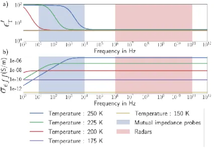
Figure 2: Dielectric constant (a) and electrical conductivity (b) of pure water ice as a function of frequency and temperature. The respective operating frequencies of mutual impedance probes and radars are indicated.
At frequencies below 104 Hz, the dielectric constant rapidly decreases with temperature, ranging from ∼ 100 at 250 K to ∼ 3.1 below 175 K. This is not the case at higher frequencies for which the relative dielectric constant of water ice can be regarded as constant, equal to about 3.1, for all temperatures. Of importance for the analysis of the data collected over a cold objects, such as comets, we highlight that below ∼ 175 K, or 150 K according to the laboratory measurements conducted by Mattei et al. (2014), the temperature does not affect the relative dielectric constant of water ice anymore, which remains equal to the high-frequency limit value, i.e. ∼ 3.1. This is due to a very long relaxation time at cryogenic temperatures.
The value of the water ice dielectric constant at low frequencies (10 Hz to 10 kHz) and for a moderately low temperature (200 K to 250 K) is especially high (between 10 and 100, as shown in Figure 2) compared to typical planetary surface materials (most of these have a relative dielectric constant lower than 10). Water ice also displays rapid increases in a relatively narrow frequency range (which depends on the temperature at ELF and VLF). This is the reason why surface mutual impedance (see section 4.4) probes are well suited to its detection.
The conductivity of water ice strongly varies with temperature at all frequencies. It decreases when the temperature decreases and progressively loses its frequency dependence. The conductivity increases with the degree of impurity of the ice.
2.2. Liquid water
The complex permittivity of liquid water can also be described by a Debye model. The static permittivity of water has a temperature dependence that has been measured experimentally and is
2. Electrical properties of natural matter
26 well modeled in the least square sense by Liebe et al. (1991) in the range of temperatures (-20 °C - 60 °C):
𝜖𝑟𝑠(𝑇) = 77.66 − 103.3× (1 − 300 𝑇(𝐾))
(32)
The high frequency limit permittivity verifies:
𝜖∞= 0.066 𝜖𝑟𝑠 (33)
and the relaxation time is dependent on temperature as described in Table 1.
Table 1: Relaxation time of liquid water as a function of temperature (from Kumbharkhane et al. 1996)
Temperature (°C) 𝝉 (ps)
0 14.8
10 10.3
25 8.7
40 6.9
The variations with temperature and frequency of the electrical properties of pure liquid water as described by equation (32) and (33) are shown in Figure 3. These equations provide a fair estimate of the dielectric constant and losses of pure liquid water. However, pure water is rarely found in natural environments and the presence of impurities may significantly affect their validity and, in particular, increase the conductivity and lower the dielectric constant. Liquid water has a very high dielectric constant (80) in the microwave domain, this is the reason why radars are well suited for its detection.
Figure 3: Dielectric constant (a) and electrical conductivity (b) of pure liquid water as a function of frequency and temperature. The respective operating frequencies of mutual impedance probes and radars are indicated.
Chapter 1: Characterizing subsurface electric properties
27
2.3. Rocks
The term “Rocks” covers a variety of compositions, porosity, density, water content and complex permittivity values. However tendencies can be derived: for example, porosity will systematically diminish the dielectric constant and the conductivity (simply because 𝜖𝑟𝑣𝑎𝑐𝑢𝑢𝑚= 1 and 𝜎𝑣𝑎𝑐𝑢𝑢𝑚= 0) while the presence of water (liquid at HF and ice at ELF) will increase the dielectric
constant. Further relationships between dielectric constant and water content have been determined empirically but for a limited domain of validity. For example, Topp et al. established in 1980 the following equation:
θ = −5.3 ∙ 10−2+ 2.92 ∙ 10−2𝜖
𝑟− 5.5 ∙ 10−4𝜖𝑟2+ 4.3 ∙ 10−6 𝜖𝑟3 (34)
with θ the volumetric liquid water content [m3∙ m−3] and 𝜖𝑟 the dielectric constant of the subsurface.
This equation can only be used in the frequency domain 500 MHz – 1 GHz.
Table 2: Dielectric constant and conductivity of common rocks and materials at two different frequencies in the ELF and HF ranges
Material 𝒇 = 𝟏𝟎𝟎 𝐇𝐳 𝒇 = 𝟏𝟎𝟎 𝐌𝐇𝐳
𝝐𝒓′ 𝝈
𝒆𝒇𝒇 (S/m) 𝝐𝒓′ 𝝈𝒆𝒇𝒇 (S/m)
Sandy soil (dry) 3.41 a N/A 2.56 a 10-5 c
Sandstone 13.0 a 10-4 b 5.20 a 1-10-3 b
Quartz 4.60 a 10-6-10-5 b 4.60 a 10-5-10-3 c
Limestone (dry) 10.4 a 10-5-10-3 b 8.56 a 10-4-10-3 b
Diorite 17 a 10-5-10-4 b 8.57 a N/A
Granite (dry) 8.47 a 10-5 b 6.68 a 10-8-10-6 c
a(Clark 1966), b(Lowrie 2007), c(Davis & Annan 1989)
Table 2 shows values of dielectric constant and conductivity of typical rocky materials. As expected, the dielectric constant is higher at low frequencies due to the additive effect of polarization mechanisms. The conductivity also tends to have lower values at lower frequencies (except for dry granite). Table 2 illustrate the wide range of electrical properties of “rocks”; on Earth this is mainly due to different water content and porosity and one must be cautious when trying to infer composition from the electrical properties. We will later discuss the mixing laws (see Section 3) that can be used to determine the complex permittivity of mixtures of rocks, water, and vacuum.
2. Electrical properties of natural matter
28 One must be cautious in using values measured for rocks to infer the composition of a subsurface as these are extremely dependent on the many parameters described above. Whenever possible a sample of material should be characterized by lab measurements.
2.4. Chondrites
The study of chondrites is of particular interest for the exploration of primitive objects such as asteroids and comets and for the origin of organic material on Earth. Chondritic material is indeed the most common material found in non-differentiated, non-metallic asteroids. Chondritic samples are generally found in meteorites (they represent 80% of the meteorites found). They are characterized by the presence of chondrules, round inclusions embedded in a matrix of different composition (see Figure 4).
Figure 4: Plane-polarized light photomicrographs of the Renazzo meteorite, the spherical inclusions are the chondrules (Weisberg et al. 1993)
We typically distinguish 15 different types of chondrites based on the composition of the matrix and chondrules (Van Schmus & Wood 1967).The two most common groups are:
- carbonaceous chondrites whose main characteristics are the presence of water, organic compounds, silicates, oxides and sulfides (Mcsween 1977)
- ordinary chondrites which contain mainly silicates but also have a non-negligible amount of iron and iron oxide (Nakamura 1974; Kallemeyn et al. 1989)
Few studies have investigated the electrical properties of chondrites. In particular Fensler et al. (1962) measured the DC conductivity and UHF (Ultra High Frequency, 300 MHz to 3000 MHz) dielectric constant and loss tangent of these two types of chondrites.
Table 3: Dielectric constant, conductivity and loss tangent of chondrites (Fensler et al. 1962)
𝝐𝒓′ 𝝈
Chapter 1: Characterizing subsurface electric properties
29
DC N/A 0.08 ∙ 10−3 - 0.20 ∙ 10−3 N/A
UHF 11.9 to 45.9 N/A 0.193 to 0.0261
Lab measurements were also performed in preparation for the CONSERT (Comet Nucleus Sounding Experiment by Radio wave Transmission) bistatic radar experiment on board the Rosetta spacecraft. Heggy et al. (2012) studied the electromagnetic properties of ordinary chondrites (LEW 85320, MET 01260 and MAC 88122 are different samples of ordinary chondrites, additional details can be found in Heggy et al. 2012) over a large range of porosities and temperatures. The results are summarized in Figure 5. We note that there seems to be no variation as a function of frequency of either the loss tangent or the dielectric constant in the frequency range from 0.5 to 90 MHz (CONSERT operates at 90 MHz). The values for the dielectric constant are in the range 4.8-6.0 for ordinary chondrites (RKP A79015 is not an ordinary chondrite).
Figure 5: Real part of the complex permittivity and loss tangent of ordinary chondrites as a function of frequency (Heggy et al. 2012)
Additional measurements of the dielectric constant of carbonaceous chondrites are reported in Kofman et al. (2015, see Figure 6). The values for the dielectric constant are in the range 2.9-3.2 (between 20 and 110 MHz) and do not show great variations with frequency.
2. Electrical properties of natural matter
30 Figure 6: Real part of the complex permittivity of carbonaceous chondrites as a function of frequency. These measurements were made on two meteoritic samples in the CONSERT frequency range (Kofman et al. 2015)
Even if their study did not extend to lower frequencies, they can be extrapolated under certain hypotheses (see Chapter 4, Section Chapter 4:5).
2.5. Lunar regolith
The complex permittivity at HF of lunar regolith sample brought to Earth by the Apollo missions was investigated by Bassett & Shackelford (1972) and Bussey (1978). The values found are reported in Table 4 showing an increasing dielectric constant with frequency (except for the last value) which is unexpected (see section 2.2). This could be explained by the small number of measurements or by the fact that they were performed in the frame of two different studies.
Table 4: Dielectric constants of lunar soil from Bassett & Shackelford (1972) and Bussey (1978).
Frequency (GHz) 𝝐𝒓′
2.0 2.04
9.375 2.10
18.0 3.71
24.0 3.18
We note that the values are higher than that of carbonaceous chondrites but lower than that of ordinary chondrites.
2.6. Martian analogs
The electromagnetic properties of Martian analogs have been extensively studied in support of two radar sounding experiments: SHARAD/Mars (SHAllow RADar) Reconnaissance Orbiter and
Chapter 1: Characterizing subsurface electric properties
31
MARSIS/Mars (Mars Advanced Radar for Subsurface and Ionosphere Sounding) Express experiments (Paillou et al. 2001; Heggy et al. 2001; Williams & Greeley 2004; Stillman & Olhoeft 2008; Stillman et al. 2010; Elshafie & Heggy 2013). Figure 7 shows the dielectric constant and loss tangent of the mars simulant JSC-Mars-1 (Allen et al. 1979) analog as function of temperature and frequency (Simões et al. 2004; Simões et al. 2007). We note an increase of the dielectric constant as the frequency decreases and a decrease in the dielectric constant and loss tangent as the temperature decreases.
Figure 7: Dielectric constant and loss tangent for the JSC-Mars-1 analog with 1% volumetric water and 54% porosity for 6 different temperatures in the 20 Hz – 10 kHz frequency range (Simões et al. 2004)
2.7. Europa crust analog
Europa, one of Jupiter’s moons, is of great interest for the search of life, or at least habitable environment in the Solar System. The surface of Europa is one of the youngest of the solar system. Its crust is composed of silicates-water ice mixture probably overlying a liquid water ocean and the potential presence of thermal vents suggests that conditions similar to those in which life emerged on Earth could exist in this ocean (Chyba et al. 2000). Future missions to Europa and, in particular, the JUICE (JUpiter ICy moons Explorer, ESA) and Europa Clipper (NASA), include ground penetrating radars designed to probe Europa’s crust (thought the chances of detection of the underground ocean are very small). the reasons for which the electromagnetic properties of Europa’s icy crust were investigated was to estimate the attenuation of the electromagnetic signal and the ability of the instrument to probe depths of the order of several kilometers or a few tens of kilometers. Pettinelli et al. (2016) performed dielectric measurements on ice/MgSO4·11H2O mixtures, a possible composition
3. Mixing laws
32 Figure 8: Dielectric constant (a and c) and imaginary part of the relative permittivity (c and d) of Europa’s ice crust analog for different MgSO4.11H2O/H2O ratios, a) & b): pure water ice c) & d): 32 % of MgSO4.11H2O. (from Pettinelli et al. 2016). The
grey areas represent the limit of detection of the instrument.
The results, presented in Figure 8 show the real and imaginary parts of the complex permittivity of mixtures as a function of ratio of MgSO4/H2O, temperature and frequency. As expected
both the real and imaginary parts increase with lower frequencies and higher temperatures. The presence of MgSO4.11H2Oaffects mainly, though moderately (compare Figure 8a to Figure 8c), the
real part by changing its frequency dependence. The presence of MgSO4.11H2O introduces moderate
additional losses (compare Figure 8b to Figure 8d). In order to retrieve the permittivity of pure MgSO4.11H2O,Pettinelli et al. (2016) used a mixing law relating the permittivity of the mixture to the
permittivity of the 2 phases and the fraction of MgSO4.11H2O. In the next section, we will present the
most commonly used mixing laws and the hypotheses behind them.
3. Mixing laws
Mixing laws can be used to estimate the electrical properties of planetary surfaces when they consist of a heterogeneous mixture of different compounds and/or phases. They generally apply when the heterogeneities are sufficiently small (a conservative rule of thumb is that the size of the heterogeneities has to be smaller than a tenth of the wavelength, which implies that mixing laws are more accurate at lower frequencies). Numerous mixing laws have been proposed (see Sihvola (1999) for a complete review), We will present here the most common formulas found in literature.
Chapter 1: Characterizing subsurface electric properties
33
The effective relative permittivity of a homogeneous matrix with small spherical inclusions (Figure 9) can be estimated using the Maxwell-Garnett mixing rule of Effective Medium Theory (Bohren & Huffman 1998):
𝜖𝑟𝑚𝑖𝑥𝑡𝑢𝑟𝑒 = 𝜖𝑟𝑚+ 3𝑓𝜖𝑟𝑚 𝜖𝑟𝑖− 𝜖𝑟𝑚
𝜖𝑟𝑖+ 2𝜖𝑟𝑚− 𝑓(𝜖𝑟𝑖− 𝜖𝑟𝑚)
(35)
where 𝜖𝑟𝑚and 𝜖𝑟𝑖 are the complex relative permittivities of the inclusions and the matrix respectively,
and 𝑓 the volume fraction of the inclusions. This law satisfies well the two limits:
𝑓 → 0, 𝜖𝑟𝑚𝑖𝑥𝑡𝑢𝑟𝑒→ 𝜖𝑟𝑚
𝑓 → 1, 𝜖𝑟𝑚𝑖𝑥𝑡𝑢𝑟𝑒 → 𝜖𝑟𝑖
Figure 9: Spherical inclusions in a homogeneous matrix, the size of the spherical inclusions has to be smaller than a tenth of the wavelength of the electromagnetic wave (Sihvola 2000).
The Maxwell-Garnett mixing rule treats one material as the matrix (host material) in which other materials (the guest material) are embedded in the form of small inclusions. However, this model is not symmetric as the host and guest materials do not contribute on an equal basis to the effective permittivity. This is the main shortcoming of this law: it relies on a good assumption of which material is the host and which is the guest. In some cases, this assumption is straightforward but in other, and in particular when the volume fraction of inclusions is close to 0.5, the choice of the host and guest material can have significant impact on the estimate of the mixture permittivity as illustrated by Figure 10.
3. Mixing laws
34 Figure 10: Dielectric constant of a liquid water/water ice mixture at HF (𝝐𝒓′𝒍𝒊𝒒𝒖𝒊𝒅= 𝟖𝟎 & 𝝐𝒓′𝒔𝒐𝒍𝒊𝒅= 𝟑. 𝟐) as inferred with
equation (35). The orange curve represents the case of liquid water inclusions in water ice and the blue curve represents the case of water ice inclusions in liquid water. The mixing law is verified in the extreme cases 𝒇𝒊𝒄𝒆= 𝟎 and 𝒇𝒊𝒄𝒆= 𝟏 but between
0 & 1 the dielectric constant is dependant on the choice of matrix/inclusions. It is especially inefficient when the volumetric fraction of inclusions is close to 50%.
Equation (35) can be generalized for a medium with multiple spherical inclusions embedded in the host matrix as follows:
𝜖𝑟𝑚𝑖𝑥𝑡𝑢𝑟𝑒 = 𝜖𝑟𝑚+ 3𝜖𝑟𝑚 ∑ 𝑓𝑛𝜖𝜖𝑟𝑖,𝑛− 𝜖𝑟𝑚 𝑟𝑖,𝑛+ 2𝜖𝑟𝑚 𝑁 𝑛=1 1 − ∑ 𝑓𝑛𝜖𝜖𝑟𝑖,𝑛− 𝜖𝑟𝑚 𝑟𝑖,𝑛+ 2𝜖𝑟𝑚 𝑁 𝑛=1 (36)
where 𝜖𝑟𝑖,𝑛 is the complex permittivity and 𝑓𝑛 the fraction of the 𝑛𝑡ℎ inclusion type. Equation (36)
satisfies well the limit:
∑ 𝑓𝑛 𝑁
𝑛=1
→ 0, 𝜖𝑟𝑚𝑖𝑥𝑡𝑢𝑟𝑒→ 𝜖𝑟𝑚
However, when ∑𝑁𝑛=1𝑓𝑛= 1, i.e. when there is no matrix the mixture relative permittivity still
depends on 𝜖𝑟𝑚.
The Bruggeman mixing formula is a corrected version of the Maxwell-Garnett formula that does not have the same shortcoming when considering multiphase mixtures (Sihvola 2000):
∑ 𝑓𝑛(𝜖𝑟𝑖,𝑛− 𝜖𝑟𝑚 𝜖𝑟𝑖,𝑛+ 2𝜖𝑟𝑚) = 0
𝑁
𝑛=1
(37)
We further emphasized that the use of the mixing laws in medium of non-null imaginary part of the relative permittivity is valid only under the condition that the loss mechanisms are the same in the inclusions and in the matrix. In the special case where the matrix has a dielectric constant of 𝜖𝑟𝑚
Chapter 1: Characterizing subsurface electric properties
35
and the inclusions are purely conductive (with a conductivity 𝜎𝑒𝑓𝑓𝑖 ) then the global conductivity of the medium can be written (Sihvola 2000):
𝜎𝑚𝑖𝑥𝑡𝑢𝑟𝑒 = 9𝜖𝑟𝑚 2 𝑓𝜎 𝑒𝑓𝑓𝑖 2𝜖𝑟𝑚2 +𝜎𝑒𝑓𝑓𝑖 2 𝜔2 (38)
The Maxwell-Garnett and Bruggeman formulas are not suitable for dense materials (Sihvola 2000). In these cases, it has been shown that is it more reliable to use the following power law approximation (Sihvola 2000; Zhou et al. 2008):
𝜖𝑟𝛼𝑚𝑖𝑥𝑡𝑢𝑟𝑒 = ∑ 𝑓𝑛𝜖𝑟𝛼𝑛 𝑁
𝑛=1
(39)
with 𝛼 the mean depolarization factor and 𝜖𝑟𝑛the relative permittivity of the n
th phase type. The
depolarization factor typically takes two values: ½ in the Birchak formula (Birchak et al. 1974) or 1/3 in the Landau-Lifshitz-Looyenga's formula (Landau et al. 1984).
Rather than taking a fixed value for the relative permittivity of the mixture, it is more conservative to determine a range of values that encompasses all estimates from previously presented formulas. In 1962, Hashin & Shtrikman (1962) defined an upper and lower bound to the range by reworking the Maxwell-Garnett formula (for a 2 phase material):
𝜖𝑟𝑚𝑖𝑛𝑚𝑖𝑥𝑡𝑢𝑟𝑒 = 𝜖 𝑚+ 𝑓 1 𝜖𝑟𝑖− 𝜖𝑟𝑚+ (1 − 𝑓)(2𝜖𝑟𝑚) (40) 𝜖𝑟𝑚𝑎𝑥𝑚𝑖𝑥𝑡𝑢𝑟𝑒 = 𝜖 𝑖+ 1 − 𝑓 1 𝜖𝑟𝑚− 𝜖𝑟𝑖 +2𝜖𝑓 𝑟𝑖 (41)
These bounds correspond to the two cases presented in Figure 10 where we at turn take one of the phases as the matrix and the other as the inclusion. In the case of a three-phase mixture the same formulas can be used by taking alternatively each phase as the matrix and the other two as inclusions. The effective permittivity of the mixture can safely be assumed to lie between the maximum and minimum values. For illustration Figure 11 presents the effective permittivity of the mixture as calculated by the laws mentioned above. We observe that all estimates are included between the Hashin and Shtrikman bounds. These bounds, though probably over conservative, are good tools to avoid the mis-estimation of the effective permittivity of heterogeneous subsurfaces
4. Methods for the characterization of subsurface electric properties
36 Figure 11: Estimate of the dielectric constant of a liquid water mixture with water ice spherical inclusions using different mixing laws. To be noted is that the Hashin-Shtrikman estimates bound all the others.
As a conclusion, the available mixing laws have their limits and only apply well in specific conditions. A safe assumption is to consider that the relative permittivity of the mixture can be found between the Hashin-Shtrikman bounds. It is recommended, when possible, to directly measure in laboratory the complex relative permittivity of mixtures rather than trying to apply a mixing law. The frequency range reliability of these formulas is dependent on the size of the inclusions: as mentioned previously a conservative rule of thumb is that the size of the inclusions must remain smaller than a tenth of the wavelength (Sihvola 2000). In the case of Mutual Impedance Probes (MIP) the wavelength is very high, making the use of mixing laws justified for this type of instrument.
4. Methods for the characterization of subsurface electric
properties
The relative permittivity of the subsurface of planetary objects can be measured with a variety of methods in situ or by remote sensing. We will first present methods that can only be used on or close to the surface, i.e. in situ. Then, we will describe the radar technique, a technique suitable for many different configurations of operation. Lastly, we will present the passive microwave radiometry which has only been used on orbiters. Other methods exist and this list is not exhaustive.
4.1. Vertical Electrical Sounding (VES)
Historically the first electromagnetic sounding method, the resistivity method patented by Wenner (1916) consists in using a DC generated current to measure the effective apparent resistivity (inverse of the effective apparent conductivity) of the subsurface. The general configuration of operation is presented in Figure 12 where two transmitting electrodes (A and B) deliver a DC current