Experimental analysis of image quality for an horizontal overwater propagation

HAL Id: hal-02480011

https://hal.archives-ouvertes.fr/hal-02480011

HAL is a multi-disciplinary open access archive for the deposit and dissemination of sci-entific research documents, whether they are pub-lished or not. The documents may come from teaching and research institutions in France or abroad, or from public or private research centers.

L’archive ouverte pluridisciplinaire HAL, est destinée au dépôt et à la diffusion de documents scientifiques de niveau recherche, publiés ou non, émanant des établissements d’enseignement et de recherche français ou étrangers, des laboratoires publics ou privés.

Experimental analysis of image quality for an horizontal

overwater propagation

Hubert Beaumont, Claude Aime, Eric Aristidi, Henri Lanteri

To cite this version:

Hubert Beaumont, Claude Aime, Eric Aristidi, Henri Lanteri. Experimental analysis of image quality for an horizontal overwater propagation. SPIE’s 1996 International Symposium on Optical Science, Engineering, and Instrumentation, 1996, Denver, United States. pp.244, �10.1117/12.254172�. �hal-02480011�

Experimental analysis of image quality for an horizontal overwater propagation H. Beaumont, C. Aime, E. Aristidi and H. Lantéri

Département d'Astrophysique. URA 709 du CNRS Université de Nice Sophia-Antipolis. Parc Valrose 06108 Nice Cedex2 France

ABSTRACT

The effect of atmospheric turbulence on the imaging of scenes, for an horizontal propagation of the light over a distance of 20 km, 15 meters above the sea surface, was analyzed at visible wavelength using a 20 cm telescope. Point-sources images were recorded during the night, and the Fried parameter r₀ was derived lead-ing to values ranglead-ing from 1.5 to 3.6 cm. A very high level of scintillation was observed. Studies of correla-tions between close-by sources lead to a very small domain of isoplanatism. Daytime observacorrela-tions of an extended source are also performed; an image motion of small spatial coherent length seems to be drawn by an horizontal wind producing wave-like distortion of horizontal lines and boiling-like of vertical ones.

1. INTRODUCTION

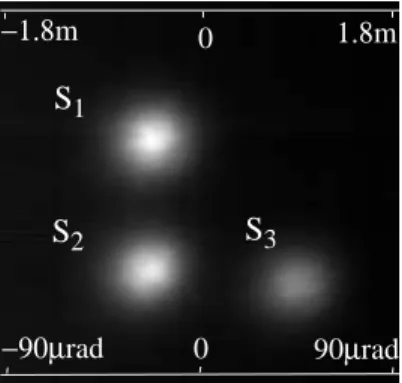
We report in this paper a study of the effects of atmospheric turbulence on the imaging of scenes, for an horizontal propagation of the light over a distance of 20 km, 15 meters above the sea surface. The data mate-rial is the result of a series of observations of images obtained at the focus of a 20 cm telescope and analysed at visible wavelengths with a CCD camera of high sensitivity and variable integration time. Observations were made by night, on point-source targets (fig. 1), and in day time on a complex extended source. The results reported here mostly concerns night-time observations.

Fig 1: Average of 800 instantaneous images of the three sources, distants one another from 170cm, corresponding to an angle of 85µrad for the target set at 20km

of the observer.

The procedure we used to quantify the effects of the atmospheric turbulence for this horizontal propaga-tion is mainly derived from those used in astronomy for site testing. We make use of blurring and image motion models and speckle transfer functions. Several quantities such as C_n2, Fried's parameter r₀ or scintil-lation rate are obtained.

After a brief description of the site and of the observational setup in Section 1, Section 2 describes the blurring, image motion and scintillation effects of point source targets. These low frequency visible features of the effect of turbulence are interpreted in terms of the Fried's parameter. Results on the domain of isopla-natism are also given there. Information about temporal and spatial correlation are retrieved in Section 3 from a speckle interferometry analysis of the image. Finally, the result of day time observations of a complex extended source are reported in Section 4 and a conclusion is drawn in Section 5.

−90µrad 0 90µrad

1.8m

−1.8m ₀

S₁

2. QUALIFICATION OF IMAGE QUALITY USING GLOBAL OBSERVATION.

The presence of atmospheric turbulence degrades the images, and it has long been known that increasing the size of a telescope beyond a certain limit does not improve the visual observation conditions. The atmo-sphere is considered to impose a filtering of the spatial frequencies present in an incident wave, thus limiting the effective resolving power of a ground-based telescope. The definition of image quality, which is expressed by the size of the smallest discernable detail in the image, is thus related uniquely to the state of the atmosphere irrespective of the telescope in use.

Fried1 introduced a parameter r₀ which provides a measure of image quality and can be defined as the telescope diameter which, in the absence of atmospheric turbulence, would give the same image resolution as a telescope of infinite aperture in the presence of turbulence. The parameter r₀ may be interpreted as well as the diameter of coherent portions of the perturbed wavefront incident on the entrance pupil of the tele-scope. For a given telescope, the value of the Fried parameter is enough to quantify the apparent effects called blurring and image motion.

Assuming isoplanatism2, the relationship between the intensity in the focal plane i(x,y) and the illumina-tion of an object o(x,y) in the presence of turbulence can be written as a convoluillumina-tion product:

where t represents time and x, y the position. The function r(x, y, t) is the instantaneous point spread function (PSF) of the atmosphere - instrument ensemble, for which an unresolved bright object appears at any given moment as a distribution of dark and bright spots called speckles. The angular extent of the speck-les is approximately limited to 2.5 λ/r₀. The analysis of the speckle phenomenon will be described in Sec-tion 3.

During long exposures, the time-average of r(x, y, t) drawns the speckles phenomenon and the averaged transfer function acts as a low pass filter, so that only the low frequency information present in the signal is transmitted3. Without entering into any theoretical analysis, we give thereafter a simple heuristic explana-tion of these effects. We start first with the instantaneous image.

The speckles are spread in the image plane over a random surface r_t(x,y) whose instantaneous shape depends on the coherence zones present on the pupil at time t. Their characteristic size can be associated with the blurring, and their transfer function is described by the so called “short- exposure” image as described by Fried, which is actually a long time exposure image corrected for image motion. From one instant to another, r_t(x,y) changes in contrast and moves in the image plane by a factor related to the mean gradient of the phase errors present in the incident wave at the telescope pupil. This image motion decreases when the size of the telescope increases4. The overall, time-averaged value of r_t(x,y) constitutes the long time exposure point spread function R(x,y) as defined by Fried and related directly to r₀.

In Fried's theory, there is a consistency between the raw long time exposure point spread function, the image corrected for motion and the image motion itself. Given the size of the telescope, these three mea-sures should be all related to r₀ and to a coefficient α that allows to take into account the relative importance of amplitude and phase perturbations of the wave front. Our analysis makes it possible to check the validity of Fried's models. It is what we describe in subsection 2.1 and 2.2. Another important global parameter for an observation is the rate of scintillation of the image, which is simply obtained in our experiment by a mea-sure of the whole intensity observed from a source. It is described in subsection 2.3. An important informa-tion may be obtained from the simultaneous observainforma-tion of several sources, that is the isoplanatism angle. We derive this information from joint analysis of image motion and scintillation of close by sources. The results are given in subsection 2.2 and 2.3.

In this paper, we make plenty use of the parameter r₀, but it may also be interesting to make use of the i x y t

(

, ,

)

=

(

,

)

(

, ,

)

refractive index structure C_n2. For spherical waves, Fried's r₀ parameter is related to C_n2 by the relation5:

where h is the distance of a turbulent layer and dh an element of thickness, L is the distance between the object and the observer and k is the optical wave number.

In the case of an horizontal propagation we may considere that C_n2(h) has a constant value over the opti-cal path6, and eq.2 reduces to:

This relation will be used to relate r₀ and C_n2 values in the following of this communication.

2.1 Determination of Fried's parameter r₀ from blurring measurements.

This section presents a measurement made among a large set of data were we measured Fried parame-ter's values between 1.5cm up to 3.6cm. As an example we choose to present especially the one we found to be the more representative for marine turbulence conditions.

We give the values of r₀ from blurred observations of PSF's with and without correction of image motion. Fried gives his results at the level of the Optical Transfer Function (OTF), Fourier transform of the PSF.

For long exposure time and monochromatic observations, the expression of the OTF is:

where τ₀(f) is the diffraction-limited OTF of the telescope, that can be written as the autocorrelation function of the telescope pupil. The PSF can be obtained as the inverse two-dimensional Fourier transform of this expression. We shall denote this PSF as r_LE (x, y).

The second approach consists of using Fried's model for images corrected for image motion. Fried assumes that the image motion follows a Gaussian distribution in the focal plane. He deduces from this assumption that eq. 4 is the result of a filtering by a Gaussian law in the Fourier plane. The corresponding short exposure time MTF, in the sense of Fried, can be written as1:

where D is the diameter of the imaging optics and α is a parameter that may vary from 1, when only eq.2 r₀ 2.1 1.46k2 Cn2

( )

−

(

)

∫

=

=

( )

( )

−

=

( )

( )

−









₍

₋

_⁄

₎

=

phase effects are considered (near field), to 0.5 when amplitude and phase effects are both important (far field). According to Fried1, the parameter α is a function that varies with f; it may be taken as a constant for given experimental conditions. The difference between the two extreme cases can be made by a comparison between the diameter of the telescope D and the quantity (Lλ)1/2, where L is the length of the propagation path through the turbulent medium. The parameter α takes the value 1 for D>>(Lλ)1/2 corresponding to the near field case and the value 0.5 for D<<(Lλ)1/2 corresponding to the far field case. Our experimental condi-tions are typically in the intermediate case, (Lλ)1/2 being of the order of 10cm for a telescope diameter D=20cm, and we may expect to find a value of α lying in the range 0.5 to 1.

As for the above relation 4, the corresponding short time exposure PSF r_SE(x, y) can be obtained as the inverse two-dimensional Fourier transform of eq.5. In fact, there is a problem for the raw application of this formula and its inversion for α=1. Indeed, in eq.5, the term (1-α(λf/D)1/3) of the exponential reduces to zero when f reaches the cut-off frequency D/λ and, consequently, makes the exponential term equal to 1 while it should tend toward zero there. In fact Fried's correction factor is valid only for low frequency values. We used eq. 5 for a limited range of f values, limiting the correcting factor (1-α(λf/D)1/3) to a minimum value of 0.1.

If no a priori assumptions are made on the relative importance of amplitude and phase effects, the fit between theory and experiment in the short exposure case requires the determination of the two parameters r₀ and α. Our approach was to trust the r₀ value obtained in the long exposure experiment and use it in the short exposure case to deduce the α value that best fit the observations.

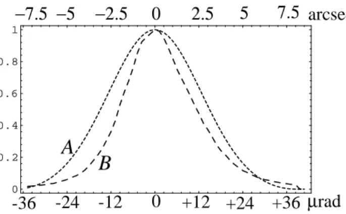
The comparison between data and models was made using a set of 800 images recorded around midnight in clear air and windy conditions. A slice of the average of the raw images and a slice of the average of the recentered images are represented in fig. 2.

Fig 2: Comparison between slices of a raw long exposure image (short dotted line A) and the same observation corrected for image motion, called short exposure image in Fried's

terminology (large dotted line B).

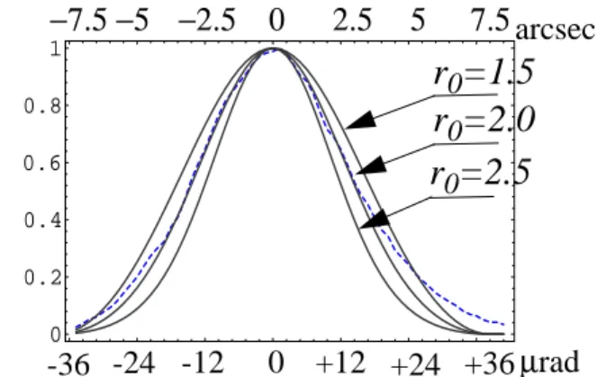
These curves are then compared with the corresponding theoretical models in the next two figures. In fig. 3, curve A of fig.2 i. e., the LTE experimental result is compared with a set of LTE PSFs obtained by a 2D Fourier Transform of eq.4 for various r₀ values. The best fit, in the least square sense, is obtained for r₀=2cm (C_n2=1.94 10-15 m-2/3). 0 10 20 30 40 50 60 0 0.2 0.4 0.6 0.8 1 Coupe de donn335

-12

+12

-24

+24

-36

0

+36

µ

rad

0

−2.5

−5

−7.5

2.5

5

7.5

arcsec

A

B

Fig 3: Comparison between a slice of a long exposure image (dotted line) with Fried's model for different values of r₀.

The best fit (dotted line) is obtained for r₀= 2cm (Cn2= 1.94 10-15 m-2/3).

In fig.4, curve B of fig.2, i. e. the STE experimental result is compared with a set of STE PSFs obtained by a 2D Fourier Transform of eq.5, for a fixed r₀ value of 2cm and variable α values from 0.5 to 1. The best fit in the least square sense is obtained for α=0.6

Fig 4: Comparison between a slice of a short exposure image with Fried's model for r₀= 2cm (Cn2= 1.94 10-15m-2/3) and different values of the α parameter

The optimal value of α is about 0.6.

2.2 Determination of Fried's parameter r₀ from image motion measurements.

The image motion can be directly measured from the set of images as the wandering of the photocenter of each short exposure image. Histograms of the horizontal and vertical motions are given in fig.5. The image motion presents an overall amplitude of 40µrad, equivalent in the object plane to about 80cm. There is a spread of the image motion slightly larger in the horizontal direction than in the vertical one, the stan-dard deviations σ being respectively of 6.8µrad and 6.6 µrad for the two directions.

0 10 20 30 40 50 60 0 0.2 0.4 0.6 0.8 1 Coupe de donn335

-12

+12

-24

+24

-36

0

+36

0

−2.5

−5

−7.5

2.5 5

7.5

_arcsec

µ

rad

r

=1.5

r

=2.0

r

=2.5

-12

+12

-24

+24

-36

0

+36

0

−2.5

−5

−7.5

2.5 5

7.5

arcsec

µ

rad

α

=1.0

α

=0.5

Fig 5:Histograms of the position of the photocenter of an unresolved source: Left, Vertical image motion; Right horizontal image motion.

The unit interval on the abscisse axis represents a 1.2µrad shift. The zero is set at the overall average position.

Assuming isotropy, the standard derivations σ of this Gaussian distribution is related to the observational conditions by:

This result is drawn from relations 7.54 and 7.47 of Roddier7, assuming identical variance of the angle of arrivals in horizontal and vertical directions. The coefficient α is used here to drop the near-field approxi-mation used by Roddier.

A quite good consistency is found between measurements and the theoretical curve for r₀=2cm and α=0.6 leading to σ=6.7µrad. The comparisons are shown in fig.6.

Fig 6: Comparison between the image motion histogram (doted line) and the Gaussian law corresponding to r₀= 2cm, or Cn2= 1.94 10-15 m-2/3 (full line).

Left: vertical image motion; right: horizontal image motion. 1 2 3 4 5 6 7 8 91011121314151617181920212223242526272829303132333435 0.2 0.4 0.6 0.8 1 1234567891011121314151617181920212223242526272829303132333435 d335viation horizontale 0.2 0.4 0.6 0.8 1

0

6.5

0

6.5

-6.5

-6.5

-12

12

18.5

-12

12

-18.5

-18.5

18.5

0

0

-1.3

1.3

-1.3

1.3

-2.7

2.7

-2.7

2.7

-4

4

-4

4

µ

rad

arcsec

σ

_0.18

_α

λ

D

( )

λ

r

( )

⋅

≈

_{eq. 6}

-12

+12

-24

+24

-36

0

+36

0

−2.5

−5

−7.5

2.5

5

7.5

µ

rad

arcsec

0

−2.5

−5

−7.5

2.5

5

7.5

µ

rad

-12

+12

-24

+24

-36

0

+36

a)

b)

2.3 Correlation of image motion

Our target made of three points sources separated from 1.7m made it very easy to check the correlation of image motions between the sources. As recently discussed by Beran and Oz-Vogt6, a simple condition of isoplanatism may be to impose that the propagation of the light coming from two points sources remains with an horizontal distance much less than r₀. This condition is far to be verified in our experiment, and we must expect the image motions to be uncorrelated.

The procedure we used to check this point was to represent the probability density function (PDF) of the difference of observed positions between two close-by sources. There are two opposite cases. If the sources are viewed within an angle lower than the isoplanatic angle, their image motion should be identical. The PDF of differences of positions should be represented by a simple point at the true difference of position of the sources.

If the sources have a separation angle much greater than the isoplanatic angle their motion become uncorrelated. In that case, we expect that the PDF of their difference of position becomes equal to the convo-lution product of their individual motion law of probability. In such a case, assuming for the image motion a Gaussian distribution of standard deviation σ (eq.6), we expect to obtain a Gaussian PDF of standard devia-tion σ_∗∗=σ√2 for the differences of positions.

The comparison between experimental data and the expected theoretical model is made in fig. 7. We have represented the differences between the observed positions of sources S₁, S₂ and S₃ of fig. 1. The observed 2D histograms are compared with the Gaussian PDF corresponding to the uncorrelated case by drawing a circle of diameter D =2 √2σ2_** log(2) of 22.2µrad that should contain 50% of the differences of positions. The obtained results (54.2% for D₁-D₂, 54.6% for D₂-D₃, and 47.5% for D₁-D₃) are roughly con-sistent with the assumption of uncorrelated image motions and we must conclude that the condition of isoplanatism is not satisfied for the 1.7m separation. However, the results obtained for D₁-D₂ and D₂-D₃, corresponding to the 1.7m separation might be consistent with a very small residual rate of coherence that is no more visible for the histogram corresponding to the difference of displacement D₁-D₃ corresponding to a separation of 2.38 m. Moreover, these histograms slightly depart from the expected theoretical isotropic dis-tribution. There is a spread in the direction of the sources.

Fig 7: Differences of observed positions of the 85µrad separated sources.

From left to right: along vertical (S₁-S₂), horizontal (S₃-S₂) and diagonal (S₁-S₃) baseline. The circle superimposed to the figure represent the limit of 2D Gaussian PDF such that the two dimensional integral is 0.5. The measured values are 54.6% for (D₁-D₂), 54.2% for (D₃-D₂) and

47.5% for (D₃-D₁).

As a result, we found that the isoplanatic angle was much less than the separation angle of the sources. We note as well, that the fluctuation in the longitudinal direction (parallel to the base) are larger than in the transverse direction (orthogonal to the base). One should note that such a differential method does not take into account correlated displacements of images caused by large scale phenomena. For instance it cannot measure the effect of a convective cell of dimensions larger or equal to the separation of the source moving in the source plane or also of a convective cell of the dimension of our pupil moving in the pupil plane.

0

0

-60µrad -60µrad -60µrad 0

0

0

2.4 Scintillation-Isoplanatic Angle

We made scintillation measurements for a single source, and analysed the correlation that exists between close by sources. The scintillation of a source produced by the atmospheric turbulence is measured as the variation of the intensity received by a point like detector located on the impinging wavefront8.

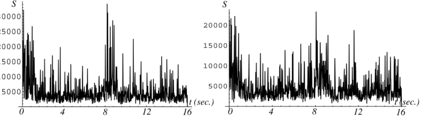
The measurement we performed is made in the focal plane of the telescope. It consists of measuring the whole intensity received from a point source by integrating the intensity of the whole PSF. This corresponds in practice to the integration of a domain of 0.1mrad centered on the source. As a consequence, we can only measure the resulting scintillation of the light integrated over the entrance aperture of the telescope. Fig. 8 shows the evolution of the received intensity as a function of time, for a total duration of 16 seconds, sam-pled at the standard video sample of ∆t_s= 20ms.

Fig 8: Scintillation: comparison of integrated irradiance of two sources 170cm (85µrad) spaced. The sample rate, ∆t_s, is the video standard 20ms sample.

N=800 measurements are represented corresponding to 16 seconds of time.

We observed very strong fluctuations and a comparison with the theory expectation is indicated below. To quantify the strength of turbulence, the theory of optical scintillation uses the scintillation index defined as the ratio of the variance of the intensity to the square of its mean:

We measured σ_I2 values of the order of 0.75. This value is very high if we consider the integration effect of large aperture. According to Bass et al.9, it is possible to recover the magnitude of the pupil averaging effect through a coefficient A defined as:

where σ_I2(D) is the variance of the relative irradiance fluctuation measured with a pupil size of diameter D and σ_I2(0) the one measured with a point-like detector.

To obtain the value of A, we used the curve given by Bass et al. ( fig. 3 of reference 9). Depending of the value we assume for the inner scale l₀, we can deduce that A range between 0.2 and 0.3. In that case, the observed σ_I2(D) value of 0.75 corresponds to possible σ_I2(0)values ranging between 2.5 and 3.75. If we use

200 400 600 800 5000 10000 15000 20000 200 400 600 800 5000 10000 15000 20000 25000 30000 8 4 12 16 t (sec.) 16 12 8 4 0 0 t (sec.) S S

σ

〈

S

〉

−

〈 〉

S

S

〈 〉

=

_{eq. 7}

eq. 8

A

σ

_{( )}

_D

σ

_{( )}

₀

=

the variance of the log amplitude7 σ_χ2, with σ_I2 = 4σ_χ2, we derive that this later quantity varies between 0.93 and 0.625. This possible variation is well inside the interval of values( π2/24, 1) defined by Churnside8 for the saturation domain. According to fig. 4 of Hill and Clifford10, it is possible to locate our measured point either in the bump or in the beginning of the saturation zone. We can exclude the weak turbulence regime. Indeed, a raw application of the Rytov model for a spherical wave would give a σ_χ2 value of the form:

Taking for C_n2 the value measured in subsection 2.1, this relation would have given the inconsistent value of 2.86 for σ_χ2, and therefore the weak turbulence regime can be excluded.

The variation of the integrated intensity coming from two sources is shown in figure 8 as a function of time. Strong uncorrelated fluctuations are visible from a sample to another, leading us to conclude that the scintillation correlation time is much smaller than 20 ms of time, as expected11.

Generally, one recognize periods of strong fluctuations of the two sources (for example in the zone 0 to 2 seconds, and just after 8 seconds) and periods of relatively quieter conditions clearly showing the non sta-tionarity of the phenomenon.

As we did for the image motion in the former section, we also studied the correlation of scintillation between two close-by sources. This comparison is performed using the couples of sources 1.70m (85µrad) spaced whose scintillation is shown in fig. 8 One can note the uncorrelated fluctuation of the two sources directly in this representation. This appears clearly in the correlation diagram shown in fig. 9, together with the regression lines.

Fig 9: Correlation diagram of close by sources with the two linear regression lines.

The rate of correlation is very weak, of the order of 60% to 70%, depending on the observations. As a result, we concluded that the scintillation isoplanatism domain is less than 1.7m for this 20km horizontal propagation.

3. TEMPORAL AND SPATIAL CORRELATION.

The results obtained in the former section can be verified and completed using a speckle analysis of instantaneous images. Let us first give a very short description of speckle observations.

The speckle technique developed by Labeyrie11 in astronomy is based on the fact that short exposure images presents bright features of the size of the Airy disc of the telescope. The problem is to know how

eq. 9

σ

_0.124k

L

C

=

short must be the exposure time to observe this phenomenon. The characteristic time for a modification of the speckle's shape is called the “boiling“ time12, by reference to the visual appearance of the speckle image. Speckle boiling times are generally found of the order of 5 to 20 ms in astronomy. The image detection sys-tem we have is not fast enough to sample in time this evolution, since our data recording is based on the standard television rate of 50 images/sec. We can however modify the integration time of each image, and therefore check the effect on the resulting image, or more conveniently, on the power spectra.

In order to estimate t₀, we performed records with several exposure times, such records allow us to com-pare the different power spectrum and then to conclude about t₀.

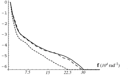
As the exposure time decreases, the energy at high spatial frequencies in the image increases but also the noise. An optimum can be found when the exposure time becomes of the order of the correlation time of the turbulence. It is then possible to distinguish the treshold due to the correlation time of the turbulence. Fig.10 show a slice of power spectra computed for 10, 8 and 4 ms. These power spectrum are cleaned from noise bias.

Fig 10: Comparison between power spectra obtained with different exposure times. Short doted line: exposure time of 10ms; Long doted line: exposure time 8ms.

Full line: exposure time:4ms.

We note that power spectra we obtained at 8 and 4 ms are close enough to assess a correlation time less or equal to 8ms. We generally processed data recorded with 4ms exposure time.

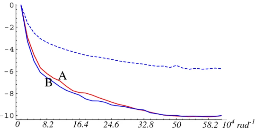
We have also checked the isoplanatism domain for the speckle experiment by computing the cross spec-trum between instantaneous images of the form < τ₁(f) τ*₂(f)>, where τ₁(f) and τ₂(f) are the Fourier Trans-form of the speckle patterns simultaneously produced by the sources S₁ and S₂ at the telescope focus. The symbol “*” stands for complex conjugate. This curve is reproduced in fig. 11 where it is compared with a cross spectrum obtained between images separated in time by 8seconds, and that we expect to be fully uncorrelated. The image power spectrum is also represented.

10 20 30 40 50 60 -6 -5 -4 -3 -2 -1 0

f (

Fig 11: Comparison between the power spectrum of a source (dotted line), the cross spectrum of instantaneous point sources (A) 1.7 m separated and the cross spectrum obtained for the same point sources, but separated in time by 8 seconds (B). There is a residual correlation for the

instantaneous images.

The results support the conclusion derived in section II. In a first approximation, PSFs corresponding to point sources separated by 1.7m are uncorrelated, as it can be seen from the comparison between <τ₁(f) τ*

2(f)> and <|τ(f)|2>. However, we cannot exclude some residual correlation, since the cross spectrum

corre-sponding to simultaneous images presents slightly more power in the high frequencies than the one com-puted for long time lagged images. It may be also interesting to note that the default of isoplanatism does not influence the OTF in the low frequency range.

4. DAYTIME OBSERVATIONS.

Daytime observation were made using as object source a rectangular target of dimension 4x3 m repre-sented in fig.12. Records were done in the afternoon, from 1 to 6 pm during nine days, from September 26th to November 13th when the air's transparency was satisfactory. Indeed, the daytime observations are strongly affected by the turbidity phenomenon, so that observation was impossible during about 74% of the time. In good condition of transparency we measured r₀ values from 3.6cm to less than 0.5cm. Typical conditions are found to be of the order of 1.5cm. Furthermore, we observed distortions of our rectangular object in a way similar to what is currently observed by solar astronomers on the solar limb at sunset. There is a general per-turbation of the image, producing wavelike distortions along horizontal edges and some kind of boiling like distortion for the verticals edges. These distortions seem to be drawn by the wind.

Fig 12: Day-time image of an extended object represented on a panel of

4 metres long and 3 metres high observed at a distance of 20 km with a 20 cm telescope. The effects of wavelike distorsionsdescribed in the body of the

communication are visible only when looking to a movie.

5 10 15 20 25 30 -10 -8 -6 -4 -2 0 8.2 16.4 24.6 32.8 50 58.2 104 rad-1 0

B

A

5. CONCLUSION

We have reported in this paper the result of a series of observations of the effects of the atmospheric turbulence on the imaging of scenes, for an horizontal propagation of the light over a distance of 20km, 15 meters above the surface of the sea. The image formed at the focus of a telescope was analyzed at visible wavelength with a CCD camera. Observations were made during the night and on daytime.

During the night, a target made of three point sources was used. The characterisation of image quality was first made using global observations of blurring, image motion and scintillation of these point sources. The parameter of Fried r₀ was deduced from the raw long time exposure point source image and the one corrected for image motion. A typical value of 2cm was found for r₀ using Fried's theory for blurring. The image motion was directly measured as the wandering of the photocenter of each short exposure image. This measurement shows standard deviations of about 6.7 µrad, slightly larger in the horizontal direction than in vertical one. The value r₀ derived from image motion alone is in agreement with the former one for a Fried's coefficient α of 0.6 corresponding to intermediate conditions between far field and near field. These observations were completed by scintillation measurements. These measurements were obtained by simply integrating the image of a point source at the focus of the 20cm diameter telescope. We found an integrated scintillation index of the order of 0.75, which corresponds to a saturation mode for the intensity of the wave at the telescope aperture.

The use of several point sources made it possible to check the isoplanatism angle. This was made from image motion and scintillation measurements of close by sources. Although theory predicts a very small isoplanatic domain, of the order of r₀ in the target plane, a very weak residual correlation was found between sources separated by 1.7m

This analysis was completed using speckle measurements. An estimate of the boiling time was obtained from the analysis of the power spectrum of images recorded with different integration times. A typical value of 4ms seems to be sufficient to freeze the speckle image. The r₀ values obtained from speckle measurements confirmed the previous ones for which global observation were used. Speckle analysis also confirmed the measurements concerning the residual correlation for the isoplanatic domain at 1.7m.

The daytime observations reported here are the results of a preliminary approach; they already show clearly the very poor seeing conditions and the importance of the turbidity phenomenon. However, rather good images were observed during some short periods.

6. ACKNOWLEDGMENT

We would like to thanks Alexandre Robini for the help given in the construction of the instrumental device. Thanks are also due to Gilbert Ricort and to Paul Massiani, Marco Barilli and Alessandro Barducci for assistance during the observations.

7. REFERENCES

1. Fried D L 1966 J. Opt. Soc. Am. 56 pp 1372-1379 2. Goodman J W 1985 Statistical Optics

3. Korff D, Dryder G, and Miller M G 1972 Opt. Commun. 5 187

4. Ziad A, Borgnino J, Martin F,Agabi K 1994 A&A, Vol. 282 pp 1021-1033 5. Tofsted D H 1991 SPIE 1487 372

6. Beran M J and Oz-Vogt J 1994 Progress in Optics Vol. XXXIII 319-388

7. Roddier F 1981 Progress in Optics Vol. XIX, ed E. Wolf,editor (North-Holland) pp 281-376 8. Churnside J H 1990 N.O.A.A.

9. Bass E, Lackovic B D and Andrews L C 1995 Optical Engineering 34 10. Hill R J and Clifford S F 1981 J. Opt. Soc. Am. 71

11. Labeyrie A 1970 Astron. Astrophys. 9, pp 85-87 12. Roddier F, Gilli J M, Lund G 1982 J. Optics, 13-5