HAL Id: hal-01790292
https://hal.archives-ouvertes.fr/hal-01790292
Submitted on 11 May 2018
HAL is a multi-disciplinary open access
archive for the deposit and dissemination of
sci-entific research documents, whether they are
pub-lished or not. The documents may come from
teaching and research institutions in France or
abroad, or from public or private research centers.
L’archive ouverte pluridisciplinaire HAL, est
destinée au dépôt et à la diffusion de documents
scientifiques de niveau recherche, publiés ou non,
émanant des établissements d’enseignement et de
recherche français ou étrangers, des laboratoires
publics ou privés.
Pivot Routing Improves Wireless Sensor Networks
Performance
Nancy Rachkidy, Alexandre Guitton, Michel Misson
To cite this version:
Nancy Rachkidy, Alexandre Guitton, Michel Misson. Pivot Routing Improves Wireless Sensor
Net-works Performance. Journal of NetNet-works, Academy Publisher, 2012. �hal-01790292�
Pivot Routing Improves Wireless Sensor
Networks Performance
Nancy El Rachkidy
(1,2), Alexandre Guitton
(1,2), Michel Misson
(3,2)(1) Clermont Universit´e, Universit´e Blaise Pascal, LIMOS, BP 10448, F-63000 Clermont-Ferrand, France (2) CNRS, UMR 6158, LIMOS, F-63173 Aubi`ere, France
(3) Clermont Universit´e, Universit´e d’Auvergne, LIMOS, BP 10448, F-63000 Clermont-Ferrand, France Emails:{nancy,guitton,misson}@sancy.univ-bpclermont.fr
Abstract—Nowadays, wireless sensor networks (WSNs) are used in several applications such as environmental monitoring. When network size and data rate increase, congestion becomes as an important issue, especially when an emergency situation generates alarm messages in a specific area of the network. In this paper, we describe the pivot routing protocol named PiRAT, which avoids congested paths by using intermediate pivot nodes. Simulations show that PiRAT has better performance than previous protocols in terms of packet loss, end-to-end delay, congestion and node overload. Moreover, we show that the load-balancing ability of PiRAT allows it to benefit from nodes having independent low duty cycles.
Index Terms—Pivot routing, congestion, packet loss, end-to-end delay, node usage, load-balancing.
I. INTRODUCTION
Most wireless sensor networks (WSNs) are composed of cheap battery-powered devices that are able to sense their environment and to communicate with each other in a wireless manner. Their low-cost and energetic autonomy has enabled environmental monitoring applications to emerge in the recent years. For instance, WSNs have been used for wildlife tracking [1] and monitoring [2]. In order to last for years with the current technology, it is crucial to save nodes energy in a WSN. As the radio module of a sensor node generally needs several times more energy than its processor [3], many researchers have focused on implementing energy-efficient communication protocols, where sensor nodes go to sleep mode periodically.
In a typical monitoring application (such as in forest fire monitoring), a WSN is deployed over a large area. Sensor nodes sense the environment periodically and report their measurements to a sink. In order to reduce the amount of packets sent, many strategies can be used. Sensor nodes usually refrain from sending packets when their new measurement is close to the previous [4]. However, unexpected changes in the environment (such as the detection of a fire) yield to the generation of high data-rate, bursty traffic from all the sensor nodes of the neighboring area. Most of the data being forwarded to the same sink, high contention is likely to occur along the path from the sources to the destination. In such a scenario, the network might experience high latency and high loss-rate, which is not acceptable in an emergency scenario. Thus, it is very important to design
communi-cation protocols that can reduce the latency or loss-rate in the case of bursty traffic. Additionally, high loss-rate might cause a large number of retransmissions, which causes congestion. Minimizing the congestion is therefore an important issue.
In this paper, we describe the PiRAT protocol [5], designed to route alarms (or more generally, packets from a limited region to a dedicated sink) using intermediate pivot nodes, thus reducing congestion. The contributions of the paper are three-fold. First, we propose rules to select pivots, and we compare the results obtained by our rules with the results from an optimal selection (obtained using an integer linear program). Second, we present a distributed protocol that can be used to implement the pivot selection rules. Third, we evaluate the performance of PiRAT according to several scenarios. We first simulate PiRAT behavior when all the nodes are active. Then, we discuss how PiRAT can benefit from nodes having low duty cycles, which is typical in a WSN intended to operate for years.
The rest of this paper is organized as follows. Section II presents the IEEE 802.15.4 and ZigBee standards, as well as some routing protocols used in WSNs. We present our PiRAT protocol in Section III. The pivot selection algo-rithm is described, and its results are compared with an optimal selection. Section IV compares the performance of the shortcut routing protocol with PiRAT when all the nodes of the network are active simultaneously. Section V emphasizes the benefits of PiRAT as the duty cycle of the nodes decreases. Finally, we conclude our work in Section VI.
II. STATE OF THE ART
IEEE 802.15.4 and ZigBee are the main standards for low-rate wireless personal area networks. They are suitable for WSNs and are commercially available, which makes them good candidates for monitoring applications. After briefly describing these standards, we present the existing routing protocols that are relevant to our study. A. IEEE 802.15.4 and ZigBee standards
The IEEE 802.15.4 standard [6] describes the physical layer (PHY) and the medium access control sublayer (MAC) of a low-power wireless personal area network.
IEEE 802.15.4 is used to interconnect ultra low-cost sensors, actuators, and processing devices [7], [8]. This standard is based on a topology composed of several coordinators (called full-function devices in the standard) and several end-devices (called reduced-function devices in the standard). One of the coordinator initiates the network, it is referred to as the personal area network (PAN) coordinator. IEEE 802.15.4 operates in two modes: the beacon-enabled mode and the non beacon-enabled mode.
The ZigBee standard [9] mainly defines the speci-fication of the upper layers of a low-power wireless personal area network, based on top of the lower layers defined in IEEE 802.15.4. It describes how the network can form a tree topology (called the cluster-tree), where coordinators are internal nodes of the tree and end-devices are its leaves. ZigBee also defines the allocation of logical addresses (referred to as short addresses) to nodes and the routing protocol. To compute these addresses, each node of the network has to know the values of three parameters: Cm, Rm, and Lm. Cm is the maximum
number of children for a coordinator. Rmis the maximum
number of children (among the Cmchildren) that can be
coordinators. Lm is the maximum depth of the tree. The
root of the tree topology is known as PAN coordinator. a) Hierarchical tree routing protocol: The hierar-chical tree routing protocol is the protocol defined by ZigBee when the distributed address assignment mecha-nism is used. Every coordinator has its own address space. Packets are routed according to the tree structure in the following way. End-devices only forward their packets to their parent coordinator. Given the short address d of a destination, a coordinator has to determine whether d is in its address space or not. If d is not in its address space, the coordinator simply forwards the frame to its parent. If d is in the address space of the coordinator, the coordinator has to determine whether d is one of its child end-devices, or to which of its children coordinators the address belongs to.
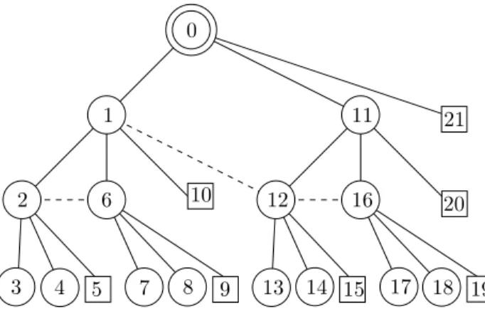
Let us consider the topology shown on Figure 1. The solid lines represent hierarchical links, while the dashed lines represent links with the neighbors. The PAN coordinator of the network is represented by a double circle, coordinators by circles and end-devices by squares. Let us suppose that a packet is sent from end-device 9
to coordinator 14. End-device 9 sends the packet to its
parent, which has address 6. Coordinator 6 determines
that the destination is not in its address space so it sends the packet to its parent, which has the address
1. Coordinator 1 sends the packet in turn to its parent,
which has the address0. Coordinator 0 (which is the PAN
coordinator) has to determine if destination14 is within
its address space[0; 20] or not. Then, the coordinator has
to determine if the destination is one of its children, or if the packet has to be sent to an intermediate child router. Here, coordinator 0 detects that destination 14 is within
the address space [11; 20] of its child 11, so it forwards
the packet to coordinator 11. Similarly, coordinator 11
determines that14 is within the address space [12; 15] of
its child router12, and forwards the packet to coordinator 12. Finally, coordinator 12 determines that destination 14
is one of its child coordinators. Coordinator12 sends the
packet to the destination14.
The main drawback of the hierarchical tree routing protocol is that routing paths are not optimal in terms of number of hops. 0 1 2 3 4 5 6 7 8 9 10 11 12 13 14 15 16 17 18 19 20 21
Figure 1. Example of tree topology with Cm = 3, Rm = 2 and
Lm= 3.
B. Shortcut tree routing protocol
The shortcut tree routing protocol [10] improves the hierarchical tree routing protocol by using the information stored in one-hop neighbor tables. The shortcut protocol also relies on the distributed address assignment mecha-nism. In this protocol, when a node generates or receives a packet for a destination d, it examines its neighbor table. For each neighbor, the node computes the distance along the tree from this neighbor to the destination of the packet (which can be computed locally based on the addresses of the neighbor and of d). Then, the node chooses as next hop the neighbor providing the shortest path to this destination. Note that this choice of neighbor can shortcut the tree topology.
Figure 1 illustrates also an example of the shortcut routing protocol. Let us consider the same example stud-ied for the hierarchical tree routing protocol, i.e. end-device9 generates a packet to send to coordinator 14. For
each neighbor, 9 computes the expected distance to the
destination14. However, it has only one neighbor which
is its parent 6, so it sends the packet to 6. Therefore, 6
computes the expected distance to the destination for each neighbor and chooses to route the packet to the neighbor that guarantees the smallest path to the destination. For neighbor2, the expected path is (2, 1, 0, 11, 12, 14) and
the distance is 5. For neighbor 1, the expected path is (1, 0, 11, 12, 14) and the distance is 4. For neighbors 7, 8,
and9 the expected distance is 6. Therefore, coordinator 6
sends the packet to1. 1 in turn examines each of its
neigh-bors. For neighbor0, the expected path is (0, 11, 12, 14)
and the distance is 3. For neighbor12, the expected path
is (12, 14) and the distance is 1. For neighbors 2, 6,
packet to its neighbor12 which shortcuts the tree. Finally,
coordinator12 detects that the destination 14 is one of its
neighbors, and sends the packet directly to it.
C. Pivot routing
In [11], Bein proposes a centralized approach where k paths are built from the source to the destination. Each path goes through several pivots, but the distance between pivots is limited by a threshold. This algorithm requires a global knowledge of the network. Our paper proposes a distributed pivot routing protocol. We focus on the case where k = 1, but the choice of pivots is not limited
to the neighborhood of the source. In [12], the authors propose a pivot routing protocol which aims to reduce the control message overhead and extend the network lifetime. Pivot nodes are determined in the following way. The sink propagates a query and selects candidate nodes as pivots based on the distance (for instance). A node is candidate if its distance from the sink (or from a previous pivot) exceeds a threshold. Each node maintains a return path to the previous pivot (or sink). In addition, several paths can be maintained between pivots. In our approach, we use only one pivot per path. Our objective is to select pivots so that paths from sources to destinations do not overlap and do not cause congestion.
III. DESCRIPTION OFPIRAT
PiRAT (pivot routing for alarm transmissions) has been proposed in [5] as a routing protocol based on pivot nodes for alarm transmissions. It can be applied to any type of high-priority traffic generated in a local area. It works as follows. Initially, each potential source of the network identifies a pivot node for each possible destination. Instead of sending alarm messages directly to the destination, PiRAT forwards messages to the pivot first, which forwards it in turn to the destination. The role of pivot nodes is to distribute the traffic load on several nodes, rather than overloading the shortest path between the sources (generally localized in a small area) and the destination and causing congestion. PiRAT improves the shortcut routing algorithm by using diversity in routing and decreasing the congested areas in the network.
PiRAT aims to reduce the congestion induced by alarm traffic in a wireless sensor network. It provides multi-path routing to the destination. Therefore, a larger number of nodes participates in routing packets. Thus, the load is balanced among the nodes of the network.
A. Pivot selection
The performance of PiRAT is tightly related to the selection of pivot nodes. Pivot nodes should not be on the shortest path from the source to the destination, otherwise PiRAT would behave as the shortcut protocol. However, pivot nodes should not be too far away from the shortest path, as this would increase the number of hops for packets. Moreover, pivot nodes should not be too close to
the source, in order to ensure that paths do not converge too early.
In this subsection, we first present an optimal algo-rithm to select paths. This algoalgo-rithm requires a global knowledge of the topology, is centralized and needs high computational resources, which makes it unrealistic in a real deployment. Then, we present a distributed algo-rithm which only requires a local knowledge. Finally, we compare the behavior of the optimal algorithm with the behavior of our distributed algorithm, in order to validate a set of rules.
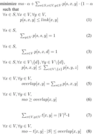
1) ILP formulation: In this part, we propose to find an optimal set of paths. Notice that we are not referring to pivot nodes here, as pivot nodes are only used in PiRAT to approximate the optimal paths. In order to find the optimal set of paths, we propose an integer linear program (ILP) formulation which computes a set of paths, one per source, such that each path is short and shares a small number of links with other paths. The trade-off between the lengths of the paths and the maximum number of links shared is given by a parameter α.
The constants of our ILP are the following. V repre-sents the nodes of the network, and link reprerepre-sents the adjacency matrix of the network. The cardinal of V is denoted by|V |. S ⊂ V is a set of sources, and d ∈ V is a
destination. The cardinal of S is denoted by|S|. α ∈ [0; 1]
corresponds to the trade-off between the lengths of the paths and the number of paths overlapping on the same link.
The variables we use are the following. p[s, x, y]
de-fines whether the link (x, y) is used by the path from s to d or not. overlap[x, y] counts the number of paths
that use the link(x, y). maxOverlap, referred to as mo
in the following, corresponds to the maximum number of paths sharing the same link. Finally, t[x, y] is a temporary
binary variable used to compute mo.
The objective function and constraints of our ILP are given on Figure 2.
In the objective function of our ILP, we weight the maximum number of shared links by α∈ [0; 1], and the
total lengths of the paths by1 − α. The first constraint of
the ILP states that the paths can only use links that are in the network. Then, we define three constraints in order to ensure that p represents the set of|S| paths, from each
node of S to the destination d. The fifth constraint com-putes the number of paths that are overlapping on a given link(x, y). The three last constraints are used to model the
non-convex function mo = maxx∈V,y∈V overlap[x, y],
using convex functions. The sixth constraint ensures that
mo is greater than or equal to every overlap[x, y]. The
seventh and the eighth constraints ensures that mo does not exceed the maximum overlap[x, y]. Indeed, notice
that as there are only|S| paths, overlap[x, y] ≤ |S|. Also
notice that only one t[x, y] is equal to 0 (due to the eighth
constraint). For all the pairs(x, y) such that t[x, y] = 1,
the ninth constraint becomes mo≤ overlap[x, y] + |S|.
For the single pair (x0, y0) such that t[x0, y0] = 0,
minimize mo· α +Ps∈S,x∈V,y∈V p[s, x, y] · (1 − α) such that ∀s ∈ S, ∀x ∈ V, ∀y ∈ V, p[s, x, y] ≤ link[x, y] (1) ∀s ∈ S, P y∈V p[s, s, y] = 1 (2) ∀s ∈ S, P x∈V p[s, x, d] = 1 (3) ∀s ∈ S, ∀x ∈ V \{d}, ∀y ∈ V \{d}, p[s, x, y] ≤ Pz∈V \{x}p[s, y, z] (4) ∀x ∈ V, ∀y ∈ V, overlap[x, y] =Ps∈Sp[s, x, y] (5) ∀x ∈ V, ∀y ∈ V, mo≥ overlap[x, y] (6) P x∈V,y∈Vt[x, y] = |V | 2 -1 (7) ∀x ∈ V, ∀y ∈ V, mo− t[x, y] · |S| ≤ overlap[x, y] (8)
Figure 2. Integer linear program for the computation of paths.
other words, mo ≥ overlap[x, y] for all (x, y) (due to
the sixth constraint), and there exists (x0, y0) such that
mo≤ overlap[x0, y0]. This corresponds to the modeling
of the maximum of a set of variables.
2) Heuristic for pivot selection: In practice, it is not realistic to find the optimal set of paths from sources to the destination using the ILP formulation. Moreover, the optimal formulation makes assumptions about the network and the nodes that are not realistic. This is why we propose here an heuristic approach based on a distributed algorithm that only requires a local knowledge. We propose to select the pivots in a large area in order to avoid the convergence of paths and thus balance the load of the traffic in the network. A sensor node is considered as a pivot when it satisfies the following criteria:
1) it is closer to the sink than to the source,
2) it is not located on the shortest path from the source to the destination,
3) it is not located on areas of the network that have a low density.
The first condition states that the pivot is closer to the destination than to the source. This is required to push the path convergence as far away as possible from the source. The second condition states that the path via the pivot does not follow the shortest path from the source to the destination, which is the most congested area. The third condition is needed as nodes in low-density areas (usually on the boundaries of the network) have less routing options than the other nodes, which reduces the
available routing diversity and increases congestion. The distance used in the previous conditions should ide-ally be the physical distance between nodes. However, as nodes have no knowledge of their geographical positions, we propose to consider the number of hops according to the shortcut tree routing as our distance. This metric is better than the number of hops computed according to the hierarchical tree routing, as it is based on the environment (through the neighbor tables) rather than on the tree topology only.
Once a source has determined a set of possible pivot nodes, it randomly chooses one of them. Then, packets are routed through this pivot.
The pivot selection protocol is the following. First, we assume that the nodes located in the potential alarm areas know in advance that they are potential sources. Thus, they initiate a pivot discovery phase by broadcasting a pivot discovery message (PDM). This message contains the distance between the source s and the destination d (computed according to the shortcut tree routing). When a node n receives a PDM, it verifies that all the three following conditions hold:
• d(s, n) > d(n, d),
• d(s, n) + d(n, d) ≥ d(s, d) + ε1, where ε1 is a
threshold chosen according to the network size,
• the number of neighbors of n is greater than a threshold ε2.
All the nodes that satisfy the three conditions are candi-dates for the pivot selection. Each candidate sends a pivot notification message (PNM) to the source to inform it that it is a potential pivot. Once the source has received a given number of PNM, or has waited for a given time duration, it chooses randomly one of them to be its dedicated pivot. If no pivot nodes are found, a new PDM is broadcasted with smaller thresholds ε1 and ε2. Notice that setting
ε1 = 0 and ε2 = 0 ensures PiRAT finds pivots on the
shortest path from the source to the destination.
3) Validation of the heuristic: We have described three ways of computing paths. The first way is to use the shortcut algorithm. The second way follows from our ILP formulation. The third way is our pivot-based heuristic. In this part, we compare the solutions found by these three approaches.
We generated a small network1 of 36 nodes deployed
according to a grid of 60m×60m. The PAN was located at
the center of the network. The communication range was set to 23 m. The destination was chosen at the top right-hand corner of the network. We generated ten independent events, each of them having a range of 13 meters. All the nodes in range of the event are sources. In our experiments, we had between two and three sources for each event. The heuristic had the following parameters:
ε1= 1 and ε2= 3.
Table I shows the average length of paths from source to destination, and the average number of overlapped links between paths, for the three algorithms. It can be seen that
1As we decided to obtain optimal solutions using a non-polynomial
the shortcut algorithm produces paths 45% longer than the ILP, on average. This is because the shortcut algorithm has only a local knowledge of the network links. Our heuristic produces paths longer than the shortcut algorithm, as pivots are introduced. However, with our choice of a small value for ε1, the paths produced by our heuristic are only
21% longer than those produced by the shortcut algo-rithm, on average. The average number of the overlapped links is 1 for the ILP: for each set of sources, the ILP was always able to find disjoint paths to the destination. This is mainly due to our limited number of sources (which was at most three), but this small number of sources is realistic for our topology. On the other hand, the average number of paths with overlapped links of shortcut was 2.5. In fifty percent of the cases, the three paths were overlapping. In the other fifty percent of the cases, only two paths have overlapped links. This happened when the sources were close to the destination. With the shortcut algorithm, paths converge quickly. Our heuristic is able to have an average number of overlapped links of 1.8. Overlapping of paths could not be completely avoided, but it could be greatly reduced compared to the shortcut algorithm.
Table I
VALIDATION OF THE PIVOT SELECTION HEURISTIC.
Algorithm Average path length Average overlapped links
Shortcut 3.2 2.5
ILP 2.2 1
Heuristic 3.9 1.8
B. Pivot discovery protocol
Our pivot selection algorithm can be implemented using two types of messages: pivot discovery message (PDM) and pivot notification message (PNM). PDMs are sent by each source. Each PDM contains the addresses of the source s and of the destination d, as pivot nodes can be different for each destination. The PDMs also contain a sequence number and the parameters (ε1 and ε2) used by
the pivot selection heuristic. Upon receiving the first PDM for a pair(s, d), a node n determines whether or not it can
be a pivot for pair(s, d). If all the rules match, n sends
a PNM back to s as a unicast message. Otherwise, the node rebroadcasts the PDM. Further PDMs for the same pair(s, d) and with a sequence number that is lower than
or equal to the one processed are discarded by node n. The PNM contains the pair (s, d) and the address of the
pivot p. If the source receives several PNMs for the same destination, it chooses randomly a pivot among all the candidates. As stated earlier, if a source does not receive PNMs after a given time, it can broadcast a new PDM with a higher sequence number, and with a weaker set of parameters.
It is also possible for the source to select a pivot without exchanging PNMs and PDMs. This is useful when the source was unable to find a pivot after having tried several set of parameters. In this case, the source can deduce from the addresses s and d a set of nodes that are close to
d (from a topological point of view), and use them as
pivots. For instance, on the example shown on Figure 1, it is possible to infer the existence of nodes0, 1, 2 and 6 from the knowledge of the address 7. Similarly, it is
possible to infer the existence of nodes 0, 1, 11 and 12
from the knowledge of address13.
We implemented our mechanism and simulated it on uniform topologies, as we varied the number of nodes from 25 to 100. We setup three random sources and computed the total number of PDMs and PNMs sent for a single destination. We averaged our results over 100 simulations. Results are shown on Figure 3. We notice that the number of PDMs and PNMs increases with the network size. This is due to the fact that, in large networks, the number of nodes participating to the pivot discovery mechanism increases. However, the number of messages does not grow too fast. On a network of 100 nodes, there are only about 200 PDMs for three sources. Indeed, potential pivot nodes do not rebroadcast PDMs. We also notice that the number of PNMs is lower than the number of PDMs. PDMs are broadcasted by every node searching for a pivot, while PNMs simply follow the path from each pivot to the source.
PDM PNM 0 50 100 150 200 20 30 40 50 60 70 80 90 100 110
Number of exchanged messages
Number of nodes
Figure 3. Average number of control messages.
IV. SIMULATION RESULTS FOR HIGH DUTY CYCLES
In this section, we describe the extensive simulations that we conducted in order to evaluate PiRAT, when all the nodes are active simultaneously. Simulations are carried out using the network simulator NS2 [13], version 2.31. We used the existing implementation of the IEEE 802.15.4 PHY and MAC layers. We used the two ray ground propagation model (with default parameters). The transmission power is set to a realistic value of 3.16
µW, which corresponds to -25 dBm, and the reception
threshold is set to 0.347412 pW (for a radio range of 30 m) or 0.195419 pW (for a radio range of 40 m). NS2 also requires the user to specify a carrier sense threshold. The carrier sense threshold could be chosen equal to the reception threshold as the IEEE 802.15.4 throughput is limited to only 250 kbps. We decided to limit the size of the alarm queue to 5 packets of 34 bytes (at the PHY layer), while the queue size for unprioritized packets
can be setup to hold more packets, typically about 15 (note that in our simulations, there are no unprioritized packets). Limiting the size of the alarm queue is imposed by the limited storage capabilities of the WSN devices. Moreover, this small size ensures that the delay of alarm packets is kept small. Increasing the alarm queue size would increase the delay, while reducing the packet loss rate.
We compared the PiRAT protocol with the hierarchical tree routing protocol, referred to as tree, and the shortcut tree routing protocol, referred to as shortcut. Each sim-ulation is performed over one hundred repetitions. We displayed the 95% confidence intervals on the following
figures. We considered a simple topology of 100 nodes, uniformly distributed in a 100 m×100 m area. Notice that
our pivot selection algorithm is suitable for any network topology. The PAN coordinator is located at the center of the area. The network parameters are defined as follows:
Cm= 5, Rm= 5 and Lm= 5. We varied the radio range
from 30 m to 40 m.
The alarm traffic is produced in the following way. First, we assume that an emergency event occurs at the bottom left-hand corner of the network. This event is detected by all the sensors located within a given radius. In our simulations, we set the detection radius to 25 m. Thus, eight nodes are sources. Notice that the event occurs in the network after all the associations are performed and the pivot selection algorithm is accomplished. There is no background traffic as we focus on the alarm traffic only. We assume that the destination is located in the top right-hand corner. All the nodes of the network participate to the multi-hop routing process. Finally, we assume that the alarm notifications last for 30 seconds and we vary the alarm data rate from 1 packet per second to 30 packets per second. Alarm notifications are produced periodically to inform the destination of the evolution of the event in a real-time manner.
In the following, PiRAT is evaluated and compared to the existing protocols according to several performance metrics:
• Packet loss: the packet loss is defined as the ratio of the number of packets successfully received by the sink over the number of packets generated by the source nodes. Thus, the packet loss ratio takes into account the losses due to collisions or queue overflows.
• End-to-end delay: the end-to-end delay is the time
interval between the transmission of a packet by the source and the reception of the same packet by the sink. Thus, the end-to-end delay only takes into account the packets that are correctly received.
• Number of hops: the number of hops is defined as the number of intermediate nodes required to forward a packet from the source to the sink. Only the packets received by the sink are considered.
• Node usage: the node usage indicates how many nodes are used in the routing process, and how many times they have to forward packets.
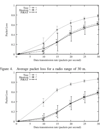
A. Packet loss
Figure 4 and Figure 5 show the mean packet loss as a function of the frequency of the alarm transmission rate with a radio range of 30 m and 40 m respectively. It is defined as the ratio of the number of packets successfully received by the destination over the number of packets generated by the source nodes. Thus, the packet loss ratio takes into account the losses due to collisions or queue overflows. We notice that the packet loss for all the protocols increases consistently with the data transmission rate. As the hierarchical routing protocol uses long paths, the probability of loosing packets is high. It can reach up to 80% for 30 packets per second and a radio range of 30 m, and up to 85% for 30 packets per second and a radio range of 40 m. The shortcut and PiRAT protocols are able to achieve lower packet loss rates by shortening the paths from the sources to the destination. They achieve only 60% packet loss rates for 30 packets per second and both radio range.
0 0.2 0.4 0.6 0.8 1 0 5 10 15 20 25 30 Packet Loss
Data transmission rate (packets per second) Tree
Shortcut PiRAT
Figure 4. Average packet loss for a radio range of 30 m.
0 0.2 0.4 0.6 0.8 1 0 5 10 15 20 25 30 Packet Loss
Data transmission rate (packets per second) Tree
Shortcut PiRAT
Figure 5. Average packet loss for a radio range of 40 m.
B. End-to-end delay
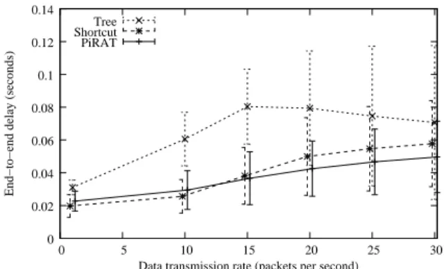
Figure 6 and Figure 7 show the mean end-to-end delay between the generation and the reception of a packet, as a function of the frequency of the alarm transmission rate with a radio range of 30 m and 40 m respectively. It is defined as the time interval between the transmission of a packet by the source and the reception of the same packet by the destination. Thus, the end-to-end delay only takes into account the packets that are correctly received.
For the hierarchical tree routing, the delay increases quickly and becomes stable after 15 packets per second.
This is due to the fact that routes are long and the number of retransmissions is high (as the packet loss is high, see Subsect. IV-A). As the data transmission rate increases, the packet loss becomes higher and several packets are dropped. The packets most likely to be dropped are those that correspond to long routes. Only packets that follow short routes enter into account when computing the end-to-end delay, which reduces the end-end-to-end delay.
For the shortcut tree routing and PiRAT, the delay increases with the data transmission rate. This is mainly due to the increasing congestion and the necessary re-transmissions. However, these two protocols outperform the hierarchical tree routing. When the alarm transmission rate is high, PiRAT has the best behavior in terms of delay. The end-to-end delay reduction of PiRAT over shortcut reaches 28% when the alarm transmission rate reaches 30 packets per second, for a radio range of 30 m, and 40% for a radio range of 40 m. When the radio range increases, shortcut and PiRAT have better performance as nodes have more neighbors to route packets to.
0 0.02 0.04 0.06 0.08 0.1 0.12 0.14 0 5 10 15 20 25 30
End−to−end delay (seconds)
Data transmission rate (packets per second) Tree
Shortcut PiRAT
Figure 6. Average end-to-end delay for a radio range of 30 m.
0 0.02 0.04 0.06 0.08 0.1 0.12 0.14 0 5 10 15 20 25 30
End−to−end delay (seconds)
Data transmission rate (packets per second) Tree
Shortcut PiRAT
Figure 7. Average end-to-end delay for a radio range of 40 m.
C. Number of hops
Table II represents the average number of hops pro-duced by the hierarchical tree routing, the shortcut rout-ing, and PiRAT protocols and the 95% confidence
in-tervals when the radius of communication range vary between 30 m and 40 m. The number of hops is defined as the number of intermediate nodes required to forward a packet from the source to the destination. Only the packets received by the destination are considered. As expected, the number of hops does not depend on the network load.
Table II
AVERAGE NUMBER OF HOPS FOR THE THREE ROUTING PROTOCOLS.
Hierarchical tree shortcut PiRAT
30 9 ± 0.5 5.5 ± 0.92 6.5 ± 0.67
40 9 ± 0.5 4.4 ± 0.7 4.8 ± 0.56
With the hierarchical tree routing, packets follow average paths of 9 hops with a 95% confidence interval of 0.5
independently from the radio range. Only the association range (which is about 20 m) is taken into account in the hierarchical tree routing protocol. The shortcut routing algorithm decreases the number of hops since it routes packets via a short path. We notice an average path length of 5.5 hops with a confidence interval of 0.92 for a radio range of 30 m and an average path length of 4.4 hops with a confidence interval of 0.7 for a radio range of 40 m. This is due to the fact that as the radio range increases, more neighbors can be used to shortcut the tree. With PiRAT, the routes are longer than those used by the shortcut tree routing, but our pivot selection algorithm ensures that the number of hops does not become too large. The average path length for PiRAT consists of 6.5 hops with a confidence interval of 0.67 for a radio range of 30 m and of 4.8 hops with a confidence interval of 0.56 for a radio range of 40 m.
D. Node usage
The node usage metric is the most important metric for PiRAT. PiRAT improves the shortcut routing algorithm by using diversity in routing and decreasing the congested areas in the network. With PiRAT, only the area around the destination is congested (see Figure 8 and Figure 9). Figure 8 and Figure 9 allow us to compare the traffic on a uniformly deployed WSN and the participation of the nodes in the routing process, when the shortcut protocol and PiRAT are used. The eight sources are nodes of
{0, 1, 2, 10, 11, 12, 20, 21}, located on the bottom
left-hand corner and the destination is node99, located at the
top right-hand corner. Links represent the packets sent between two nodes. The width of the link indicates the number of packets being sent through the link. Indeed, a thick line indicates that the link is used several times while a thin line indicates that a link is rarely used. Pivot nodes are represented using dashed circles.
Paths followed with the shortcut tree protocol (see Figure 8) tend to converge to a single path as packets become closer to the destination. This fact causes conges-tion along the common path. Moreover, as soon as one of the nodes of the path drains its energy because it has transmitted too many packets, the routes becomes inactive and the network is considered down. On the contrary, paths followed with PiRAT (see Figure 9) present more diversity. Indeed, new nodes participate in the routing process, but the traffic load is reduced for each node. PiRAT paths avoid the central area in order to reduce congestion. The probabilistic feature of PiRAT can be seen as each node uses several paths to reach a given destination (either the pivot node or the sink). While the
shortcut tree routing protocol uses21 nodes, PiRAT uses
a total of 42 nodes. Thus, PiRAT doubles the number
of nodes used, and then, it reduces the amount of the transmitted packets per node. This leads to reduce the overloaded paths and balance the energy consumption of the nodes, which greatly improves the network lifetime.
0 1 2 3 4 5 6 7 8 9 10 11 12 13 14 15 16 17 18 19 20 22 22 23 24 25 26 27 28 29 30 31 32 33 34 35 36 37 38 39 40 41 42 43 44 45 46 47 48 49 50 51 52 53 54 55 56 57 58 59 60 61 62 63 64 65 66 67 68 69 70 71 72 73 74 75 76 77 78 79 80 81 82 83 84 85 86 87 88 89 90 91 92 93 94 95 96 97 98 99
Figure 8. Node usage with the shortcut tree routing protocol.
00 00 00 00 11 11 11 11 00 00 00 00 00 11 11 11 11 11 000 000 000 000 000 111 111 111 111 111 00 00 00 00 11 11 11 11 00 00 00 00 00 11 11 11 11 11 00 00 00 00 11 11 11 11 0 1 2 3 4 5 6 7 8 9 10 11 12 13 14 15 16 17 18 19 20 22 22 23 24 25 26 27 28 29 30 31 32 33 34 35 36 37 38 39 40 41 42 43 44 45 46 47 48 49 50 51 52 53 54 55 56 57 58 59 60 61 62 63 64 65 66 67 68 69 70 71 72 73 74 75 76 77 78 79 80 81 82 83 84 85 86 87 88 89 90 91 92 93 94 95 96 97 98 99
Figure 9. Node usage with PiRAT protocol.
As we can see on Figure 8, the path from the PAN coordinator (node 45) to the sink (node 99) via the
intermediate nodes 66, 86, and 97 is overloaded. This
is due to the fact that all the packets converge to the same path. However, as it can be seen on Figure 9, the nodes used by the shortcut protocol are less solicited to route packet when PiRAT is used. With PiRAT, new nodes participate in the routing process; the traffic load is reduced for each node. Indeed, because of the diversity in routing, node 45 sends packets to nodes 47 and 75
and does not use the wireless link(45 − 66). Then, node 86 receives less packets from more nodes (56, 68, 83, 84)
than on Figure 8. However, since the destination is always the same (node99), the destination is always overloaded
with both protocols. Thus, the area around it is congested.
V. IMPROVEMENT OFPIRATFOR LOW DUTY CYCLES
In this section, we discuss about the benefits brought by PiRAT when nodes have a low duty cycle. We assume here that each node is periodically active and inactive. The activity period of nodes are independent and chosen randomly at the beginning of the simulation, as in [14]. We assume that each node knows the activity cycle of its neighbors, that is, each node can predict when any of its neighbors is going to be active or inactive. This can be achieved by having each node broadcasting to its neighbors its own activity schedule, initially. An example with a low duty cycle of 0.5 is shown on Fig. 10, which depicts the activity (in solid plain rectangles) and inactiv-ity (in striped rectangles) of three nodes. As it can be seen, the activity periods of the nodes are independent. For instance, the time during which node 1 can communicate with node 2, denoted as 1⇔2, is smaller than the whole
activity period of node 1.
000 000 000 000 000 111 111 111 111 111 0000 0000 0000 0000 0000 1111 1111 1111 1111 1111 00000 00000 00000 00000 00000 11111 11111 11111 11111 11111 0000 0000 0000 0000 0000 1111 1111 1111 1111 1111 00000 00000 00000 00000 00000 11111 11111 11111 11111 11111 0000 0000 0000 0000 0000 1111 1111 1111 1111 1111 0000 0000 0000 0000 1111 1111 1111 1111 0000 0000 0000 0000 1111 1111 1111 1111 00 00 00 00 11 11 11 11 node 1 node 2 node 3 time time time 1⇔3 2⇔3 1⇔2
Figure 10. In low duty cycles, the activity periods of nodes are
independent (which does not require synchronization).
Based on these assumptions, we adapt the MAC sub-layer in the following way. When the MAC subsub-layer examines a frame in the frame queue, it checks whether the next hop for this frame is active or not. If it is active, the MAC sublayer sends the frame to the selected neighbor. Otherwise, the MAC sublayer examines the next frame in the queue. The rationale behind this is that the next hop for the second frame in queue might be different from the next hop of the first frame in queue, and it might correspond to an active neighbor. If none of the frames of the queue can be forwarded, the MAC sublayer waits until any next hop becomes active again. This approach is a case of cross-layering, which is a commonly used technique in WSNs to improve performance [15]–[17].
When an emergency situation occurs, several messages are generated for the same destination. In the case of the shortcut protocol, when a node has several frames in its queue, all of these frames have the same next hop. Thus, our adaptation of the MAC sublayer has no effect on the shortcut protocol. However, for PiRAT, a node might have frames for different pivot nodes in its queue. Instead of being blocked because the next hop of the first frame is inactive, the node might be able to send another frame to an active neighbor.
In order to measure the benefits of this improvement, we evaluated by simulation the average waiting time before a neighbor becomes active. We varied the number of neighbors, and we activated the nodes independently. Each node is activated periodically every 2 seconds, for 50% to 100% of the time. Thus, the duty cycle of nodes varies from 0.5 to 1. With this setup, the sender is always able to be active at the same time as any of its neighbors. We computed the waiting time before the activation of the selected neighbor (which is 0 if both nodes are active at the same time). Values are averaged over 10,000 repetitions.
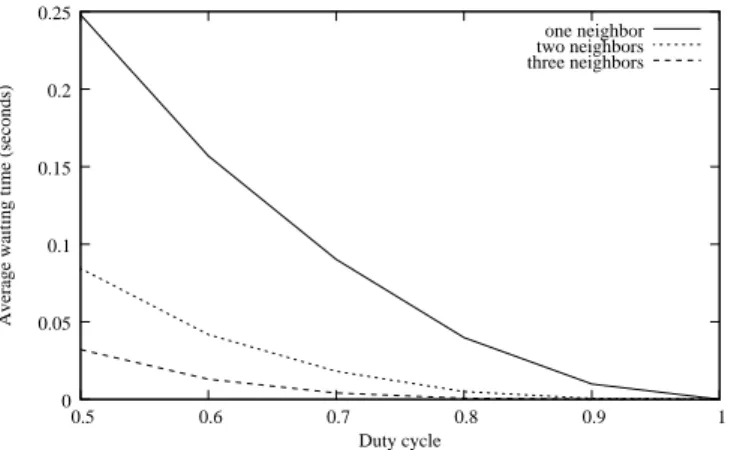
Figure 11 shows the average waiting time as a function of the duty cycle. As expected, the average waiting time decreases as the duty cycle of nodes increases. It can be noticed that this delay is not negligible, as it can reach 0.25 seconds for an duty cycle of 0.5. The main result depicted on the figure is the gain brought by allowing a node to consider two or three neighbors, rather than only one (as shortcut does). When the duty cycle is 0.5, considering two neighbors instead of only one reduces the delay by 68%. Similarly, considering three neighbors instead of one reduces the delay by 88%.
0 0.05 0.1 0.15 0.2 0.25 0.5 0.6 0.7 0.8 0.9 1 Duty cycle one neighbor two neighbors three neighbors
Average waiting time (seconds)
Figure 11. The average waiting time is greatly reduced when several
neighbors are considered.
Reducing the average waiting time is critical for a routing protocol in a low duty cycle WSN. Indeed, each node of the path delays the packet by this time (on average), as each node has to wait for the next hop to be active. This delay negatively impacts all the packets in the queue, as packets are usually processed sequentially. PiRAT, however, is less subject to this phenomenon than other protocols, due to two main reasons: (i) As PiRAT uses several intermediate pivots, the packets in the queue of a node can have different next hops, and PiRAT can thus send one of those packets as soon as the corresponding neighbor becomes active. (ii) As PiRAT balances the load on several links rather than using only a few links, it can maintain a high throughput even if the link availability is reduced due to the low duty cycle of nodes. On the contrary, a protocol which uses few links requires many packets to be sent on each link. If the link availability is reduced, a larger time is required, which decreases the overall throughput.
VI. CONCLUSIONS
When a WSN is used for a monitoring application, the presence of an emergency situation might be detected simultaneously by several sensor nodes within a limited region, which results into high data rate, bursty traffic sharing several links. We described the PiRAT protocol, which uses pivot nodes in order to avoid the congested area by balancing the load over multiple nodes. PiRAT is able to compete with the current state-of-the art protocols when all the nodes are active simultaneously. The per-formance improvement brought by PiRAT is maximized when the energy constraint of the WSN requires that sensor nodes have low duty cycles.
ACKNOWLEDGEMENT
This work has been partially supported by a research grant from the Lebanese National Council for Scientific Research (LNCSR).
REFERENCES
[1] P. Juang, H. Oki, Y. Wang, M. Martonosi, L. S. Pen, and D. Ruben-stein, “Energy-efficient computing for wildlife tracking: design tradeoffs and early experiences with ZebraNet,” ACM SIGOPS Operating Systems Review, vol. 36, no. 5, pp. 96–107, 2002. [2] T. He, S. Krishnamurthy, J. A. Stankovic, T. Abdelzaher, L. Luo,
R. Stoleru, T. Yan, L. Gu, J. Hui, and B. Krogh, “Energy-efficient surveillance system using wireless sensor networks,” in International Conference on Mobile Systems, Applications and Services, 2004, pp. 270–283.
[3] C. A. SmartRF, “CC2420 preliminary datasheet,” Chipcon, Datasheet revision 1.2, 2004.
[4] C. Lageweg, J. Janssen, and M. Ditzel, “Data aggregation for target tracking in wireless sensor networks,” in Smart Sensing and Context, ser. LNCS, no. 4272, 2006, pp. 15–24.
[5] N. El Rachkidy, A. Guitton, and M. Misson, “Pirat: Pivot Routing for Alarm Transmission in Wireless Sensor Networks,” in IEEE Local Computer Networks, 2009.
[6] IEEE 802.15, “Part 15.4: Wireless medium access control (MAC) and physical layer (PHY) specifications for low-rate wireless personal area networks (WPANs),” ANSI/IEEE, Standard 802.15.4 R2006, 2006.
[7] J. Zheng and M. J. Lee, “Will IEEE 802.15.4 make ubiquitous network a reality? a discussion on a potential low power, low bit rate standard,” IEEE Communications Magazine, vol. 27, no. 6, pp. 23–29, 2004.
[8] E. Callaway, P. Gorday, L. Hester, J. Gutierrez, M. Naeve, B. Heile, and V. Bahl, “Home networking with IEEE 802.15.4: A develop-ing standard for low-rate wireless personal area network,” IEEE Communications Magazine, vol. 40, no. 8, pp. 70–77, 2002. [9] ZigBee, “ZigBee Specification,” ZigBee Standards Organization,
Standard ZigBee 053474r17, January 2008.
[10] T. Kim, D. Kim, N. Park, S.-E. Yoo, and T. S. L ´opez, “Shortcut tree routing in ZigBee networks,” in Proceedings IEEE International Symposium on Wireless Pervasive Computing PISWPC), February 2007, pp. 42–47.
[11] D. Bein, “Fault-tolerant k-fold Pivot Routing in Wireless Sensor Networks,” in 41st Hawaii Internation Conference on System Sciences, 2008.
[12] J. Lee, R. J.P., and H. K.J., “Efficient Routing Scheme Using Pivot Node in Wireless Sensor Networks,” in ICCS, ser. LNCS, no. 4490, 2007, pp. 574–577.
[13] “Network simulator 2,” 2002, http://www.isi.edu.nsnam/ns. [14] A. Koubaa, M. Alves, M. Attia, and A. Van
Nieuwen-huyse, “Collision-free beacon scheduling mechanisms for IEEE 802.15.4/Zigbee cluster-tree wireless sensor networks,” Polytech-nic Institute of Porto, TechPolytech-nical Report TR-061104, November 2006.
[15] I. F. Akyildiz, M. C. Vuran, and O. B. Akan, “A cross-layer protocol for wireless sensor networks,” in Annual Conference on Information Sciences and Systems, 2006, pp. 1102–1107.
[16] W. Su and T. L. Lim, “Cross-layer design and optimization for wireless sensor networks,” in International Conference on Software Engineering, Artificial Intelligence, Networking and Par-allel/Distributed Computing, 2006, pp. 278–284.
[17] K. Al Agha, G. Chalhoub, A. Guitton, E. Livolant, S. Mahfoudh, P. Minet, M. Misson, J. Rahm´e, T. Val, and A. Van Den Bossche, “Cross-layering in an industrial wireless sensor network: Case study of OCARI,” Journal of Networks, vol. 4, no. 6, pp. 411– 420, 2009.
Nancy El Rachkidy is currently working as a research assistant at LIMOS-CNRS, Clermont-Ferrand, France. She obtained her PhD in computer science in 2011, at Universit´e Blaise Pascal. She received her MSc degree in networks and computer science from the Lebanese University of Beirut, Lebanon, in 2006. Her research interests include routing and MAC protocols and cross-layering in wireless sensor networks.
Alexandre Guitton is an assistant professor at Clermont Univer-sit´e, Universit´e Blaise Pascal, France. He is doing his research at LIMOS-CNRS. He received his PhD in 2005 and his MSc in 2002 at University of Rennes I, in the field of computer networks. He has been working at Clermont Universit´e since 2007. His research interests include wireless communications, sensor networks, MAC protocols, and energy-efficiency.
Michel Misson obtained his PhD thesis in nuclear physics and his ”Habilitation `a Diriger des Recherches” (HDR) degree respectively in 1979 and 2001 both at Universit´e Blaise Pascal, Clermont-Ferrand in France. In 1983, he became a lecturer, teaching networks and system architecture in the Computer Science Department of the institute of Technology in Clermont-Ferrand. He is now Professor in the Networks and Telecom-munications Department and he manages the research team ”R´eseaux et Protocoles” of the Computer Science Laboratory of Universit´e Blaise Pascal: LIMOS-CNRS. He served on many conference committees and journals reviewing processes. He has also held a visiting position in the research Laboratory T´el´ebec in Underground Communications of Quebec Univer-sity in Abitibi-Temiscamingue (LRTCS-UQAT). His current research interests are Wireless Local Area Networks, Low Power Wireless Personal Networks, Wireless Sensor Networks real-time systems and protocol engineering.