WORKING
PAPERS
SES
N. 508
IX.2019
Direct and Indirect Effects
based on
Changes-in-Changes
Martin Huber,
Mark Schelker,
and
Anthony Strittmatter
Direct and Indirect Effects based on Changes-in-Changes
Martin Huber*, Mark Schelker*, Anthony Strittmatter+
*University of Fribourg, Dept. of Economics
+University of St. Gallen, Swiss Institute for Empirical Economic Research
Abstract: We propose a novel approach for causal mediation analysis based on changes-in-changes assumptions restricting unobserved heterogeneity over time. This allows disen-tangling the causal effect of a binary treatment on a continuous outcome into an indirect effect operating through a binary intermediate variable (called mediator) and a direct ef-fect running via other causal mechanisms. We identify average and quantile direct and indirect effects for various subgroups under the condition that the outcome is monotonic in the unobserved heterogeneity and that the distribution of the latter does not change over time conditional on the treatment and the mediator. We also provide a simulation study and an empirical application to the Jobs II programme.
Keywords: Direct effects, indirect effects, mediation analysis, changes-in-changes, causal mechanisms, treatment effects.
JEL classification: C21.
We have benefited from comments by conference/seminar participants at the Universities of Melbourne, Sydney, Hamburg, and Lisbon, the Luxembourg Institute of Socio-Economic Research, and the 2019 Meetings of the International Association for Applied Econometrics. Addresses for correspondence: Martin Huber, Chair of Applied Econometrics - Evaluation of Public Policies, Uni-versity of Fribourg, Bd. de P´erolles 90, 1700 Fribourg, Switzerland,[email protected]. Mark
Schelker, Chair of Public Economics, University of Fribourg, Bd. de P´erolles 90, 1700 Fribourg, Switzerland, [email protected]. Anthony Strittmatter, Swiss Institute for Empirical
Eco-nomic Research (SEW), University of St. Gallen, Varnb¨uelstr. 14, 9000 St. Gallen, Switzerland,
1
Introduction
Causal mediation analysis aims at disentangling a total treatment effect into an indirect effect operating through an intermediate variable – commonly referred to as mediator – as well as the direct effect. The latter includes any causal mechanisms not operating through the mediator of interest. Even when the treatment is random, direct and indirect effects are generally not identified by simply controlling for the mediator without accounting for its potential endogeneity, as this likely introduces selection bias, seeRobins and Greenland (1992).
This paper suggests a novel identification strategy for causal mediation analysis based on changes-in-changes (CiC) as suggested by Athey and Imbens (2006) for evaluating (total) average and quantile treatment effects. We adapt the approach to the identification of the direct effect and the indirect effect running through a binary mediator. The outcome variable must be continuous and is required to be observed both prior to and after treatment and mediator assignment as it is the case in repeated cross sections or panel data. The key identifying assumptions imply that the continuous outcome is strictly monotonic in unobserved heterogeneity and that the distribution of unobserved heterogeneity does not change over time condi-tional on the treatment and the mediator (the latter assumption is also known as stationarity). Given appropriate common support conditions, this permits identify-ing direct effects on subpopulations conditional on the treatment and the mediator states, even if both treatment and mediator assignment are endogenous.
Augmenting the assumptions by random treatment assignment and weak mono-tonicity of the mediator in the treatment allows for causal mediation analysis in subpopulations defined upon whether and how the mediator reacts to the treat-ment. Specifically, we show the identification of direct effects among those whose mediator is always one (always-takers in the denomination of Angrist, Imbens, and Rubin,1996) and never one (never-takers) irrespective of treatment assignment, re-spectively. Furthermore, we identify the total, direct, and indirect treatment effects
any set of assumptions, we discuss the identification of both average and quantile direct and indirect effects. We note that if appropriately weighted, the respective av-erage effects among compliers, always-takers, and never-takers add up to the avav-erage direct and indirect effects in the population.
Identification in the earlier mediation literature typically relied on linear models for the mediator and outcome equations and often neglected endogeneity issues, see for instanceCochran(1957),Judd and Kenny(1981), andBaron and Kenny (1986). More recent contributions use more general identification approaches based on the potential outcome framework and take endogeneity issues explicitly into considera-tion. Examples include Robins and Greenland (1992), Pearl (2001), Robins (2003),
Petersen, Sinisi, and van der Laan (2006), VanderWeele (2009), Imai, Keele, and Yamamoto (2010), Hong (2010), Albert and Nelson (2011), Imai and Yamamoto
(2013), Tchetgen Tchetgen and Shpitser (2012), Vansteelandt, Bekaert, and Lange
(2012), and Huber (2014). The vast majority of the literature assumes that the covariates observed in the data are sufficiently rich to control for treatment and mediator endogeneity. Also in empirical economics, there has been an increase in the application of such selection on observables approaches, see for instance Simon-sen and Skipper (2006), Flores and Flores-Lagunes (2009), Heckman, Pinto, and Savelyev(2013),Huber(2015),Keele, Tingley, and Yamamoto(2015),Conti, Heck-man, and Pinto (2016), Huber, Lechner, and Mellace (2017), Bijwaard and Jones
(2019),Bellani and Bia (2018),Huber, Lechner, and Strittmatter(2018), andDoerr and Strittmatter(2019). Comparably few studies in economics develop or apply in-strumental variable approaches for disentangling direct and indirect effects, see for instance Fr¨olich and Huber (2017), Powdthavee, Lekfuangfu, and Wooden (2013),
Brunello, Fort, Schneeweis, and Winter-Ebmer (2016) and Chen, Chen, and Liu
(2017). Our paper provides another, CiC-based identification strategy that neither rests on selection on observables assumptions nor on instrumental variables for the treatment or the mediator.
pop-ulation, a smaller strand of the literature uses the principal stratification framework ofFrangakis and Rubin (2002) to investigate effects in subpopulations (or principal strata) defined upon whether and how the mediator reacts to the treatment, see
Rubin (2004). This approach has been criticized for typically focussing on direct effects on populations whose mediator is constant (i.e. always- and never-takers) rather than decomposing direct and indirect effects on compliers and for consider-ing subpopulations rather than the total population, see VanderWeele (2008) and
VanderWeele (2012). Deuchert, Huber, and Schelker (2017) suggest a difference-in-differences (DiD) strategy that alleviates such criticisms. Identification relies on a randomized treatment, monotonicity of the (binary) mediator in the treatment, and particular common trend assumptions on mean potential outcomes across principal strata. The latter imply that mean potential outcomes under specific treatment and mediator states change by the same amount over time across specific subpopulations. Depending on the strength of common trend and effect homogeneity assumptions across principal strata, direct and indirect effects are identified for different subpop-ulations and under the strongest set of assumptions even for the total population.
Our paper contributes to this literature on principal strata effects, but relies on different identifying assumptions thanDeuchert, Huber, and Schelker(2017). While differential time trends across subpopulations are permitted, our approach restricts the conditional distribution of unobserved heterogeneity over time. The two sets of assumptions are not nested and their appropriateness is to be judged in the empirical context at hand. However, both approaches could be used simultaneously for testing the joint validity of the identifying assumptions of either method, in which case both CiC and DiD converge to the same, true average direct and indirect effects. As a further distinction to Deuchert, Huber, and Schelker (2017), our proposed method also permits assessing quantile treatment effects (QTEs) rather than average effects only.
We provide a simulation study in which we compare the CiC to the DiD approach to illustrate our identification results. We also consider an empirical application to
the Jobs II programme previously analysed by Vinokur, Price, and Schul (1995), a randomized job training intervention designed to analyse the impact of job train-ing on labour market and mental health outcomes. We investigate the direct effect of the randomized offer of treatment on a depression index, as well as its indirect effect through actual participation in the programme as mediator. The reason for investigating the direct effect is that treatment assignment could have a motiva-tion or discouragement effect on those randomly offered or not offered the training. We, however, find the direct effect estimates to be close to zero and statistically insignificant and therefore no indication for the violation of the exclusion restriction when using treatment assignment as instrumental variable for actual participation. In contrast, the moderately negative total and indirect effects on those induced to participate by assignment are statistically significant at least at the 10% level in all but one case and very much in line with the estimate obtained by instrumental variable regression.
The remainder of this study is organized as follows. Section 2 introduces the notation and defines the direct and indirect effects of interest. Section 3 presents the assumptions underlying our CiC approach as well as the identification results. Section4provides a simulation study. Section 5 provides an application to Jobs II. Section6 concludes.
2
Notation and effects
2.1
Average effects
Let D denote a binary treatment (e.g., receiving the offer to participate in a training programme) and M a binary intermediate variable or mediator that may be a func-tion of D (e.g., the actual participafunc-tion in a training programme). Furthermore, let T indicate a particular time period: T = 0 denotes the baseline period prior to the realisation of D and M , T = 1 the follow up period after measuring D and M in which the effect of the outcome is evaluated. Finally, let Yt denote the outcome of
interest (e.g., health measures) in period T = t. Indexing the outcome by the time period t ∈ {0, 1} implies that it is measured both in the baseline period and after the realisation of D and M . To define the parameters of interest, we make use of the potential outcome notation, see for instance Rubin (1974), and denote by Yt(d, m) the potential outcome for treatment state D = d and mediator state M = m in time T = t, with d, m, t, ∈ {0, 1}. Furthermore, let M (d) denote the potential mediator as a function of the treatment state d ∈ {0, 1}. For notational ease, we will not use any time index for D and M , because either is assumed to be measured at a single point in time between T = 0 and T = 1, albeit not necessarily at the same point, as D causally precedes M . Therefore, D and M correspond to the actual treatment and mediator status in T = 1, while it is assumed that no treatment or mediation takes place in T = 0.
Using this notation, the average treatment effect (ATE) in the ex-post period is defined as ∆1 = E[Y1(1, M (1)) − Y1(0, M (0))]. That is, the ATE corresponds to the effect of D on the outcome that either affects the latter directly (net of any effect on the mediator) or indirectly through an effect on M . Indeed, the total ATE can be disentangled into the direct and indirect effects, denoted by θ1(d) = E[Y1(1, M (d)) − Y1(0, M (d))] and δ1(d) = E[Y1(d, M (1)) − Y1(d, M (0))], by adding and subtracting Y1(1, M (0)) or Y1(0, M (1)), respectively:
∆1 = E[Y1(1, M (1)) − Y1(0, M (0))], = E[Y1(1, M (1)) − Y1(1, M (0))] | {z } =δ1(1) + E[Y1(1, M (0)) − Y1(0, M (0))] | {z } =θ1(0) , = E[Y1(1, M (1)) − Y1(0, M (1))] | {z } =θ1(1) + E[Y1(0, M (1)) − Y1(0, M (0))] | {z } =δ1(0) .
Distinguishing between θ1(1) and θ1(0) or δ1(1) and δ1(0), respectively, implies the possibility of interaction effects between D and M such that the direct and indirect effects could be heterogeneous across values d = 1 and d = 0.
specific subpopulations. The latter are either defined conditional on the treatment and mediator values or conditional on potential mediator values under either treat-ment states, which matches the so-called principal stratum framework ofFrangakis and Rubin (2002). As outlined in Angrist, Imbens, and Rubin (1996) in the con-text of instrumental variable-based identification, any individual i in the population belongs to one of four strata, henceforth denoted by τ , according to their potential mediator status under either treatment state: always-takers (a: M (1) = M (0) = 1) whose mediator is always one, compliers (c: M (1) = 1, M (0) = 0) whose mediator corresponds to the treatment value, defiers (de: M (1) = 0, M (0) = 1) whose medi-ator opposes the treatment value, and never-takers (n: M (1) = M (0) = 0) whose mediator is never one. Note that τ cannot be pinned down for any individual, because either M (1) or M (0) is observed, but never both.
Let ∆τ
1 = E[Y1(1, M (1)) − Y1(0, M (0))|τ ] denote the ATE conditional on τ ∈ {a, c, de, n}; θτ
1(d) and δ1τ(d) denote the corresponding direct and indirect effects. Because M (1) = M (0) = 0 for any never-taker, the indirect effect for this group is by definition zero (δn
1(d) = E[Y1(d, 0) − Y1(d, 0)|τ = n] = 0) and ∆n1 = E[Y1(1, 0) − Y1(0, 0)|τ = n] = θ1n(1) = θ1n(0) = θ1n equals the direct effect for never-takers. Correspondingly, because M (1) = M (0) = 1 for any always-taker, the indirect effect for this group is by definition zero (δ1a(d) = E[Y1(d, 1) − Y1(d, 1)|τ = a] = 0) and ∆a
1 = E[Y1(1, 1) − Y1(0, 1)|τ = a] = θa1(1) = θ1a(0) = θa1 equals the direct effect for always-takers. For the compliers, both direct and indirect effects may exist. Note that M (d) = d due to the definition of compliers. Accordingly, θc
1(d) = E[Y1(1, d) − Y1(0, d)|τ = c] equals the direct effect for compliers, δ1c(d) = E[Y1(d, 1)−Y1(d, 0)|τ = c] equals the indirect effect for compliers, and ∆c
1 = E[Y1(1, 1)−Y1(0, 0)|τ = c] equals the total effect for compliers. In the absence of any direct effect, the indirect effects on the compliers are homogeneous, δ1c(1) = δ1c(0) = δ1c, and correspond to the local average treatment effect (LATE, e.g.,Angrist, Imbens, and Rubin,1996). Analogous results hold for the defiers.
values D = d and mediator states M = M (d) = m, which are denoted by θ1d,m(d) = E[Y1(1, m) − Y1(0, m)|D = d, M (d) = m]. These parameters are identified under weaker assumptions than strata-specific effects, but are also less straightforward to interpret, as they refer to mixtures of two strata. For instance, θ11,0(1) = E[Y1(1, 0)− Y1(0, 0)|D = 1, M (1) = 0] is the effect on a mixture of never-takers and defiers, as these two groups satisfy M (1) = 0. Likewise, θ10,0(0) refers to never-takers and compliers satisfying M (0) = 0, θ10,1(0) to always-takers and defiers satisfying M (0) = 1, and θ11,1(1) to always-takers and compliers satisfying M (1) = 1.
2.2
Quantile effects
We denote by FYt(d,m)(y) = Pr(Yt(d, m) ≤ y) the cumulative distribution function
of Yt(d, m) at outcome level y. Its inverse, FY−1t(d,m)(q) = inf{y : FYt(d,m)(y) ≥ q}, is
the quantile function of Yt(d, m) at rank q. The total QTE are denoted by ∆1(q) = FY−1
1(1,M (1))(q) − F
−1
Y1(0,M (0))(q). The QTE can be disentangled into the direct quantile
effects, denoted by θ1(q, d) = FY−1
1(1,M (d))(q) − F
−1
Y1(0,M (d))(q), and the indirect quantile
effects, denoted by δ1(q, d) = FY−11(d,M (1))(q) − FY−11(d,M (0))(q).
The conditional distribution function in stratum τ is FYt(d,m)|τ(y) = Pr(Yt(d, m) ≤
y|τ ) and the corresponding conditional quantile function is FY−1
t(d,m)|τ(q) = inf{y :
FYt(d,m)|τ(y) ≥ q} for τ ∈ {a, c, d, n}. Using the previously described
stratifica-tion framework, we define the QTE condistratifica-tional on τ ∈ {a, c, de, n}: ∆τ1(q) = FY−1
1(1,M (1))|τ(q) − F
−1
Y1(0,M (0))|τ(q). The direct quantile treatment effect among
never-takers equals ∆n1(q) = FY−1
1(1,0)|n(q) − F
−1
Y1(0,0)|n(q) = θ
n
1(q). The direct quantile effect among always-takers equals ∆a
1(q) = F −1 Y1(1,1)|a(q) − F −1 Y1(0,1)|a(q) = θ a 1(q). The total QTE among compliers equals ∆c
1(q) = F −1
Y1(1,1)|c(q) − F
−1
Y1(0,0)|c(q), the direct quantile
effect among compliers equals θc
1(q, d) = F −1
Y1(1,d)|c(q) − F
−1
Y1(0,d)|c(q), and the indirect
quantile effect among compliers equals δc
1(q, d) = F −1
Y1(d,1)|c(q) − F
−1
Y1(d,0)|c(q). Finally,
and mediator states M = M (d) = m, θ1d,m(q, 1) = FY−1 1(1,m)|D=d,M (1)=m(q) − F −1 Y1(0,m)|D=d,M (1)=m(q) and θ1d,m(q, 0) = FY−1 1(1,m)|D=d,M (0)=m(q) − F −1 Y1(0,m)|D=d,M (0)=m(q),
with the quantile function FY−1
t(d,m)|D=d,M (d)=m(q) = inf{y : FYt(d,m)|D=d,M (d)=m(y) ≥
q} and the distribution function FYt(d,m)|D=d,M (d)=m(y) = Pr(Yt(d, m) ≤ y|D =
d, M (d) = m).
2.3
Observed distribution and quantile transformations
We subsequently define various functions of the observed data required for the iden-tification results. The conditional distribution function of the observed outcome Yt conditional on treatment value d and mediator state m, is given by FYt|D=d,M =m(y) =
Pr(Yt ≤ y|D = d, M = m) for d, m ∈ {0, 1}. The corresponding conditional quantile function is FY−1
t|D=d,M =m(q) = inf{y : FYt|D=d,M =m(y) ≥ q}. Furthermore,
Qdm(y) := FY−11|D=d,M =m◦ FY0|D=d,M =m(y) = F
−1
Y1|D=d,M =m(FY0|D=d,M =m(y))
is the quantile-quantile transform of the conditional outcome from period 0 to 1 given treatment d and mediator status m. This transform maps y at rank q in period 0 (q = FY0|D=d,M =m(y)) into the corresponding y
0 at rank q in period 1 (y0 = FY−1
1|D=d,M =m(q)).
3
Identification and Estimation
3.1
Identification
This sections discusses the identifying assumptions along with the identification results for the various direct and indirect effects. We note that our assumptions could be adjusted to only hold conditional on a vector of observed covariates. In
this case, the identification results would hold within cells defined upon covari-ate values. In our main discussion, however, covaricovari-ates are not considered for the sake of ease of notation. For notational convenience, we maintain throughout that Pr(T = t, D = d, M = m) > 0 for t, d, m ∈ {1, 0}, implying that all possible treatment-mediator combinations exist in the population in both time periods. Our first assumption implies that potential outcomes are characterized by a continuous nonparametric function, denoted by h, that is strictly monotonic in a scalar U that reflects unobserved heterogeneity.
Assumption 1: Strict monotonicity of continuous potential outcomes in unob-served heterogeneity.
The potential outcomes satisfy the following model: Yt(d, m) = h(d, m, t, U ), with the general function h being continuous and strictly increasing in the scalar unob-servable U ∈ R for all d, m, t ∈ {0, 1}.
Assumption 1 requires the potential outcomes to be continuous implying that there is a one-to-one correspondence between a potential outcome’s distribution and quan-tile functions, which is a condition for point identification. For discrete potential outcomes, only bounds on the effects could be identified, in analogy to the discus-sion in Athey and Imbens (2006) for total (rather than direct and indirect) effects. Assumption 1 also implies that individuals with identical unobserved characteristics U have the same potential outcomes Yt(d, m), while higher values of U correspond to strictly higher potential outcomes Yt(d, m). Strict monotonicity is automatically sat-isfied in additively separable models, but Assumption 1 also allows for more flexible non-additive structures that arise in nonparametric models.
The next assumption rules out anticipation effects of the treatment or the media-tor on the outcome in the baseline period. This assumption is plausible if assignment to the treatment or the mediator cannot be foreseen in the baseline period, such that behavioral changes affecting the pre-treatment outcome are ruled out.
Similarly,Athey and Imbens(2006) andChaisemartin and D’Haultfeuille(2018) as-sume the assignment to the treatment group does not affect the potential outcomes as long as the treatment is not yet realized.
Furthermore, we assume conditional independence between unobserved hetero-geneity and time periods given the treatment and no mediation.
Assumption 3: Conditional independence of U and T given D = 1, M = 0 or D = 0, M = 0.
(a) U ⊥⊥ T |D = 1, M = 0, (b) U ⊥⊥ T |D = 0, M = 0.
Under Assumption 3a, the distribution of U is allowed to vary across groups de-fined upon treatment and mediator state, but not over time within the group with D = 1, M = 0. Assumption 3b imposes the same restriction conditional on D = 0, M = 0. Assumption 3 thus imposes stationarity of U within groups defined on D and M . This assumption is weaker than (and thus implied by) requiring that U is constant across T for each individual i. For example, Assumption 3 is satisfied in the fixed effect model U = η + vt, with η being a time-invariant individual-specific unobservable (fixed effect) and vt an idiosyncratic time-varying unobservable with the same distribution in both time periods.
Athey and Imbens (2006) and Chaisemartin and D’Haultfeuille (2018) impose time invariance conditional on the treatment status, U ⊥⊥ T |D = d, to identify the average treatment effect on the treated, ϕ1 = E[Y1(1, M (1)) − Y1(0, M (0))|D = 1] or local average treatment effect, ϕ1 = E[Y1(1, M (1))−Y1(0, M (0))|τ = c], respectively. We additionally condition on the mediator status to identify direct and indirect effects.
For our next assumption, we introduce some further notation. Let FU |d,m(u)) = Pr(U ≤ u|D = d, M = m) be the conditional distribution of U with support Udm. Assumption 4: Common support given M = 0.
(a) U10⊆ U00, (b) U00⊆ U10.
Assumption 4a is a common support assumption, implying that any possible value of U in the population with D = 1, M = 0 is also contained in the population with D = 0, M = 0. Assumption 4b imposes that any value of U conditional on D = 0, M = 0 also exists conditional on D = 1, M = 0. Both assumptions together imply that the support of U is the same in both populations, albeit the distributions may generally differ.
Assumptions 1 to 3 permit identifying direct effects on mixed populations of never-takers and defiers as well as never-takers and compliers, respectively, as for-mally stated in Theorem 1.
Theorem 1: Under Assumptions 1–3,
(a) and Assumption 4a, the average and quantile direct effects under d = 1 con-ditional on D = 1 and M (1) = 0 are identified:
θ11,0(1) = E[Y1− Q00(Y0)|D = 1, M = 0], θ1,01 (q, 1) = FY−1
1|D=1,M =0(q) − F
−1
Q00(Y0)|D=1,M =0(q).
(b) and Assumption 4b, the average and quantile direct effects under d = 0 con-ditional on D = 0 and M (0) = 0 are identified:
θ10,0(0) = E[Q10(Y0) − Y1|D = 0, M = 0], θ0,01 (q, 0) = FQ−1
10(Y0)|D=0,M =0(q) − F
−1
Y1|D=0,M =0(q).
Proof. See AppendixA.
To identify direct effects on further populations, we invoke a conditional inde-pendence assumption that is in the spirit of Assumption 3, but refers to different combinations of the treatment and the mediator.
Assumption 5: Conditional independence of U and T given D = 0, M = 1 or D = 1, M = 1.
(b) U ⊥⊥ T |D = 1, M = 1.
Under Assumption 5a, the distribution of U is allowed to vary by treatment and mediator group, but not over time conditional on D = 0, M = 1. Assumption 5b imposes the same restriction conditional on D = 1, M = 1.
Assumption 6 is similar to Assumption 4, but imposes common support condi-tional on M = 1 rather than M = 0.
Assumption 6: Common support given M = 1. (a) U01⊆ U11,
(b) U11⊆ U01.
Assumptions 6a implies that any possible value of U in the population with D = 0, M = 1 is also contained in the population with D = 1, M = 1. Assumptions 6b states that any value of U conditional on D = 1, M = 1 exists conditional on D = 0, M = 1.
Theorem 2 shows the identification of the direct effects on mixed populations of always-takers and defiers as well as always-takers and compliers.
Theorem 2: Under Assumptions 1-2, 5,
(a) and Assumption 6a, the average and quantile direct effects under d = 0 con-ditional on D = 0 and M (0) = 1 are identified:
θ10,1(0) = E[Y1− Q11(Y0)|D = 0, M = 1], θ0,11 (q, 0) = FY−1
1|D=0,M =1(q) − F
−1
Q11(Y0)|D=0,M =1(q).
(b) and Assumption 6b, the average and quantile direct effects under d = 1 is identified conditional on D = 1 and M (1) = 1 are identified:
θ11,1(1) = E[Q01(Y0) − Y1|D = 1, M = 1], θ1,11 (q, 1) = FQ−1
01(Y0)|D=1,M =1(q) − F
−1
Y1|D=1,M =1(q).
In the instrumental variable framework, any direct effects of the instrument are typically ruled out by imposing the exclusion restriction, in order to identify the causal effect of an endogenous regressor on the outcome, see for instanceImbens and Angrist (1994). By considering D as instrument and M as endogenous regressor, θ1,01 (1) = θ10,0(0) = θ0,11 (0) = θ11,1(1) = 0 yield testable implications of the exclusion restriction under Assumptions 1-6.
So far, we did not impose exogeneity of the treatment or mediator. In the following, we assume treatment exogeneity by invoking independence between the treatment and the potential post-treatment variables.
Assumption 7: Independence of the treatment and potential mediators/outcomes. {Yt(d, m), M (d)} ⊥⊥ D, for all d, m, t, ∈ {0, 1}.
Assumption 7 implies that there are no confounders jointly affecting the treatment on the one hand and the mediator and/or outcome on the other hand. It is satis-fied under treatment randomization as in successfully conducted experiments. This allows identifying the ATE: ∆1 = E[Y1|D = 1] − E[Y1|D = 0].
Furthermore, we assume the mediator to be weakly monotonic in the treatment. Assumption 8: Weak monotonicity of the mediator in the treatment.
Pr(M (1) ≥ M (0)) = 1.
Assumption 8 is standard in the instrumental variable literature on local average treatment effects when denoting by D the instrument and by M the endogenous regressor, see Imbens and Angrist (1994) and Angrist, Imbens, and Rubin (1996). It rules out the existence of defiers.
As discussed in the AppendixC, the total ATE ∆1 = E[Y1|D = 1] − E[Y1|D = 0] and QTE ∆1(q) = FY−11|D=1(q)−F
−1
Y1|D=0(q) for the entire population are identified
un-der Assumption 7. Furthermore, Assumptions 7 and 8 yield the strata proportions, denoted by pτ = Pr(τ ), as functions of the conditional mediator probabilities given the treatment, which we denote by p(m|d) = Pr(M = m|D = d) for d, m ∈ {0, 1}
(see AppendixC):
pa = p1|0, pc= p1|1− p1|0 = p0|0− p0|1, pn= p0|1. (1)
Furthermore, Assumptions 2, 7, and 8 imply that (see AppendixC)
∆0,c = E[Y0(1, 1) − Y0(0, 0)|c] =
E[Y0|D = 1] − E[Y0|D = 0] p1|1− p1|0
= 0. (2)
Therefore, a rejection of the testable implication E[Y0|D = 1] − E[Y0|D = 0] = 0 in the data would point to a violation of these assumptions.
Assumptions 7 and 8 permit identifying additional parameters, namely the total, direct, and indirect effects on compliers, and the direct effects on never- and always-takers, as shown in Theorems 3 to 5. This follows from the fact that defiers are ruled out and that the proportions and potential outcome distributions of the various principal strata are not selective w.r.t. the treatment.
Theorem 3: Under Assumptions 1–3, 7-8,
a) and Assumption 4a, the average and quantile direct effects on never-takers are identified:
θ1n= θ1,01 (1) and θn1(q) = θ1,01 (q, 1).
b) and Assumption 4, the average direct effect under d = 0 on compliers is identified: θc1(0) = p0|0 p0|0− p0|1 θ10,0(0) − p0|1 p0|0− p0|1 θ11,0(1).
Furthermore, the potential outcome distributions under d = 0 on compliers are identified: FY1(1,0)|τ =c(y) = p0|0 p0|0− p0|1FQ10(Y0)|D=0,M =0(y) − p0|1 p0|0− p0|1c FY1|D=1,M =0(y), (3)
FY1(0,0)|τ =c(y) = p0|0 p0|0− p0|1FY1|D=0,M =0(y) − p0|1 p0|0− p0|1 FQ00(Y0)|D=1,M =0(y). (4)
Therefore, the direct quantile effect under d = 0 on compliers, θc
1(q, 0) = FY−1
1(1,0)|c(q) − F
−1
Y1(0,0)|c(q), is identified.
Proof. See AppendixD.
Theorem 4: Under Assumptions 1–2, 5, 7-8,
a) and Assumption 6a, the average and quantile direct effects on always-takers are identified:
θ1a= θ0,11 (0) and θa1(q) = θ0,11 (q, 0).
b) and Assumption 6, the average direct effect under d = 1 on compliers is identified: θc1(1) = p1|1 p1|1− p1|0 θ11,1(1) − p1|0 p1|1− p1|0 θ10,1(0).
Furthermore, the potential outcome distributions under d = 1 for compliers are identified: FY1(1,1)|τ =c(y) = p1|1 p1|1− p1|0 FY1|D=1,M =1(y) − p1|0 p1|1− p1|0FQ11(Y0)|D=0,M =1(y), (5) FY1(0,1)|τ =c(y) = p1|1 p1|1− p1|0 FQ01(Y0)|D=1,M =1(y) − p1|0 p1|1− p1|0 FY1|D=0,M =1(y). (6)
Therefore, the direct quantile effect under d = 1 on compliers θc
1(q, 1) = FY−1
1(1,1)|c(q) − F
−1
Y1(0,1)|c(q) is identified.
Proof. See AppendixE.
a) and Assumptions 4a, 6a, the total average treatment effect on compliers is identified: ∆c1 = p1|1 p1|1− p1|0 E[Y1|D = 1, M = 1] − p1|0 p1|1− p1|0 E[Q11(Y0)|D = 0, M = 1] − p0|0 p1|1− p1|0 E[Y1|D = 0, M = 0] + p0|1 p1|1− p1|0 E[Q00(Y0)|D = 1, M = 0].
Furthermore, the total quantile treatment effect on compliers ∆c
1(q) = F −1
Y1(1,1)|c(q)−
FY−1
1(0,0)|c(q) is identified using the inverse of (5) and (4).
b) and Assumptions 4a, 6b, the average indirect effect under d = 0 on compliers is identified: δ1c(0) = p1|1 p1|1− p1|0E[Q11(Y0)|D = 1, M = 1] − p1|0 p1|1− p1|0E[Y1|D = 0, M = 1] − p0|0 p1|1− p1|0 E[Y1|D = 0, M = 0] + p0|1 p1|1− p1|0 E[Q00(Y0)|D = 1, M = 0].
Furthermore, the quantile indirect effect under d = 0 on compliers δc
1(q, 0) = FY−1
1(0,1)|c(q) − F
−1
Y1(0,0)|c(q) is identified using the inverse of (6) and (4).
c) and Assumptions 4b, 6a, the average indirect effect under d = 1 on compliers is identified: δ1c(1) = p1|1 p1|1− p1|0 E[Y1|D = 1, M = 1] − p1|0 p1|1− p1|0 E[Q11(Y0)|D = 0, M = 1] − p0|0 p1|1− p1|0 E[Q00(Y0)|D = 0, M = 0] + p0|1 p1|1− p1|0 E[Y1|D = 1, M = 0].
Furthermore, the quantile indirect effect under d = 1 on compliers δ1c(q, 1) = FY−1
1(1,1)|c(q) − F
−1
Y1(1,0)|c(q) is identified using the inverse of (5) and (3).
3.2
Estimation
As in Assumption 5.1 of Athey and Imbens (2006), we assume standard regularity conditions, namely that conditional on T = t, D = d, and M = m, Y is a random draw from that subpopulation defined in terms of t, d, m ∈ {1, 0}. Furthermore, the outcome in the subpopulations required for the identification results of interest must have compact support and a density that is bounded from above and below as well as continuously differentiable. Denote by N the total sample size across both periods and all treatment-mediator combinations and by i ∈ {1, ..., N } an index for the sampled subject, such that (Yi, Di, Mi, Ti) correspond to sample realizations of the random variables (Y, D, M, T ).
The total, direct, and indirect effects may be estimated using the sample anal-ogy principle, which replaces population moments with sample moments (e.g. Man-ski, 1988). For instance, any conditional mediator probability given the treatment, Pr(M = m|D = d), is to be replaced by an estimate thereof in the sample, PN
i=1I{Mi=m,Di=d}
PN
i=1I{Di=d} . A crucial step is the estimation of the quantile-quantile
trans-forms. The application of such quantile transformations dates at least back to
Juhn, Murphy, and Pierce (1991), see also Chaisemartin and D’Haultfeuille (2018),
W¨uthrich (2019), and Strittmatter(2019) for recent applications. First, it requires estimating the conditional outcome distribution, FYt|D=d,M =m(y), by the conditional
empirical distribution ˆFYt|D=d,M =m(y) =
1 Pn
i=1I{Di=d,Mi=m,Ti=t}
P
i:Di=d,Mi=m,Ti=tI{Yi ≤
y}. Second, inverting the latter yields the empirical quantile function ˆFY−1
t|D=d,M =m(q).
The empirical quantile-quantile transform is then obtained by
ˆ
Qdm(y) = ˆFY−11|D=d,M =m( ˆFY0|D=d,M =m(y)).
This permits estimating the average and quantile effects of interest. Average effects are estimated by replacing any (conditional) expectations with the corresponding sample averages in which the estimated quantile-quantile transforms enter as
plug-in estimates. Takplug-ing θ1,01 (see Theorem 1) as an example, an estimate thereof is ˆ θ11,0(1) = Pn 1 i=1I{Di = 1, Mi = 0, Ti = 1} X i:Di=1,Mi=0,Ti=1 Yi − Pn 1 i=1I{Di = 1, Mi = 0, Ti = 0} X i:Di=1,Mi=0,Ti=0 ˆ Q00(Yi).
Likewhise, quantile effects are estimated based on the empirical quantiles.
For the estimation of total ATE and QTE, Athey and Imbens (2006) show that the resulting estimators are √N -consistent and asymptotically normal, see their Theorems 5.1 and 5.3. These properties also apply to our context when splitting the sample into subgroups based on the values of a binary treatment and mediator (rather than the treatment only). For instance, the implications of Theorem 1 in
Athey and Imbens(2006) when considering subsamples with D = 1 and D = 0 carry over to considering subsamples with D = 1, M = 0 and D = 0, M = 0 for estimating the average direct effect on never-takers. In contrast to Athey and Imbens (2006), however, some of our identification results include the conditional mediator proba-bilities Pr(M = m|D = d). As the latter are estimated with√N -consistency, too, it follows that the resulting effect estimators are again√N -consistent and asymptoti-cally normal. We use a non-parametric bootstrap approach to calculate the standard errors. Chaisemartin and D’Haultfeuille (2018) show the validity of the bootstrap approach for such kind of estimators, which follows from their asymptotic normality. For the case that identifying assumptions to only hold conditional on observed covariates, denoted by X, estimation must be adapted to allow for control variables. Following a suggestion by Athey and Imbens (2006) in their Section 5.1, basing estimation on outcome residuals in which the association of X and Y has been purged by means of a regression is consistent under the additional assumption that the effects of D and M are homogeneous across covariates. As an alternative,Melly and Santangelo (2015) propose a flexible semiparametric estimator that does not impose such a homogeneity-in-covariates assumption and show√N -consistency and asymptotic normality.
4
Simulations
To shape the intuition for our identification results, this section presents a brief simulation based on the following data generating process (DGP):
T ∼ Binom(0.5), D ∼ Binom(0.5), U ∼ U nif (−1, 1), V ∼ N (0, 1)
independent of each other, and
M = I{D + U + V > 0}, YT = Λ((1 + D + M + D · M ) · T + U ).
Treatment D as well as the observed time period T are randomized, while the mediator-outcome association is confounded due to the unobserved time constant heterogeneity U . The potential outcome in period 1 is given by Y1(d, M (d0)) = Λ((1 + d + M (d0) + d · M (d0)) + U ), where Λ denotes a link function. If the latter corresponds to the identity function, our model is linear and implies a homogeneous time trend T equal to 1. If Λ is nonlinear, the time trend is heterogeneous, which invalidates the common trend assumption of difference-in-differences models. M is not only a function of D and U , but also of the unobserved random term V , which guarantees common support w.r.t. U , see Assumptions 4 and 6. Compliers, always-takers, and never-takers satisfy, respectively: c = I{U + V ≤ 0, 1 + U + V > 0}, a = I{U + V > 0}, and n = I{1 + U + V ≤ 0}.
In the simulations with 1,000 replications, we consider two sample sizes (N = 1, 000, 4, 000) and investigate the behaviour of our change-in-changes methods as well as the difference-in-differences approach ofDeuchert, Huber, and Schelker (2017) in both a linear (Λ equal to identity function) and nonlinear outcome model where Λ equals the exponential function. To implement the change-in-changes estimators in the simulations as well as the application in Section 5, we make use of the ‘cic’ command in the qte R-package byCallaway (2016) with its default values.
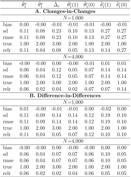
Table 1: Linear model with random treatment ˆ θn 1 θˆa1 ∆ˆc θˆ1c(1) θˆc1(0) δˆ1c(1) ˆδ1c(0) A. Changes-in-Changes N =1,000 bias 0.00 -0.00 -0.01 -0.01 -0.01 -0.00 -0.01 sd 0.11 0.08 0.23 0.10 0.13 0.27 0.27 rmse 0.11 0.08 0.23 0.10 0.13 0.27 0.27 true 1.00 2.00 3.00 2.00 1.00 2.00 1.00 relr 0.11 0.04 0.08 0.05 0.13 0.14 0.27 N =4,000 bias -0.00 -0.00 0.00 -0.00 -0.01 0.01 0.01 sd 0.06 0.04 0.12 0.05 0.07 0.14 0.14 rmse 0.06 0.04 0.12 0.05 0.07 0.14 0.14 true 1.00 2.00 3.00 2.00 1.00 2.00 1.00 relr 0.06 0.02 0.04 0.02 0.07 0.07 0.14 B. Difference-in-Differences N =1,000 bias 0.01 -0.00 -0.01 -0.01 0.00 -0.02 0.00 sd 0.11 0.09 0.14 0.14 0.12 0.19 0.10 rmse 0.11 0.09 0.14 0.14 0.12 0.19 0.10 true 1.00 2.00 3.00 2.00 1.00 2.00 1.00 relr 0.11 0.04 0.05 0.07 0.12 0.10 0.10 N =4,000 bias -0.00 -0.00 0.00 -0.00 -0.00 0.00 0.00 sd 0.06 0.04 0.07 0.07 0.06 0.10 0.05 rmse 0.06 0.04 0.07 0.07 0.06 0.10 0.05 true 1.00 2.00 3.00 2.00 1.00 2.00 1.00 relr 0.06 0.02 0.02 0.04 0.06 0.05 0.05
Note: ‘bias’, ‘sd’, and ‘rmse’ provide the bias, standard deviation, and root mean squared error of the respective estimator. ‘true’ and ‘relr’ are the respective true effect as well as the root mean squared error relative to the true effect.
(‘rmse’), true effect (‘true’), and the relative root mean squared error in percent of the true effect (‘relr’) of the respective estimators of θ1n, θa1, ∆c, θ1c(1), θ1c(0), δ1c(1), and δc1(0) for the linear model. In this case, the identifying assumptions underly-ing both the change-in-changes (Panel A.) and difference-in-differences (Panel B.) estimators are satisfied. Specifically, the homogeneous time trend on the individ-ual level satisfies any of the common trend assumptions in Deuchert, Huber, and Schelker (2017), while the monotonicity of Y in U and the independence of T and U satisfies the key assumptions of this paper. For this reason any of the estimates
in Table 1 are close to being unbiased and appear to converge to the true effect at the parametric rate when comparing the results for the two different sample sizes.
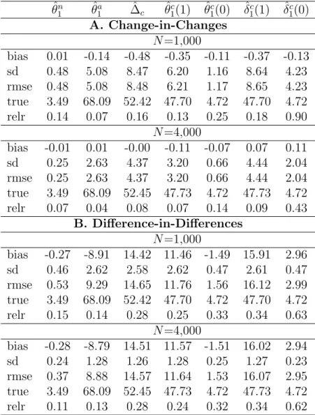
Table 2: Nonlinear model with random treatment ˆ θ1n θˆa1 ∆cˆ θˆc1(1) θˆc1(0) δˆ1c(1) δˆc1(0) A. Change-in-Changes N =1,000 bias 0.01 -0.14 -0.48 -0.35 -0.11 -0.37 -0.13 sd 0.48 5.08 8.47 6.20 1.16 8.64 4.23 rmse 0.48 5.08 8.48 6.21 1.17 8.65 4.23 true 3.49 68.09 52.42 47.70 4.72 47.70 4.72 relr 0.14 0.07 0.16 0.13 0.25 0.18 0.90 N =4,000 bias -0.01 0.01 -0.00 -0.11 -0.07 0.07 0.11 sd 0.25 2.63 4.37 3.20 0.66 4.44 2.04 rmse 0.25 2.63 4.37 3.20 0.66 4.44 2.04 true 3.49 68.09 52.45 47.73 4.72 47.73 4.72 relr 0.07 0.04 0.08 0.07 0.14 0.09 0.43 B. Difference-in-Differences N =1,000 bias -0.27 -8.91 14.42 11.46 -1.49 15.91 2.96 sd 0.46 2.62 2.58 2.62 0.47 2.61 0.47 rmse 0.53 9.29 14.65 11.76 1.56 16.12 2.99 true 3.49 68.09 52.42 47.70 4.72 47.70 4.72 relr 0.15 0.14 0.28 0.25 0.33 0.34 0.63 N =4,000 bias -0.28 -8.79 14.51 11.57 -1.51 16.02 2.94 sd 0.24 1.28 1.26 1.28 0.25 1.27 0.23 rmse 0.37 8.88 14.57 11.64 1.53 16.07 2.95 true 3.49 68.09 52.45 47.73 4.72 47.73 4.72 relr 0.11 0.13 0.28 0.24 0.32 0.34 0.62
Note: ‘bias’, ‘sd’, and ‘rmse’ provide the bias, standard deviation, and root mean squared error of the respective estimator. ‘true’ and ‘relr’ are the respective true effect as well as the root mean squared error relative to the true effect.
Table 2 provides the results for the exponential outcome model, in which the time trend is heterogeneous and interacts with U through the nonlinear link func-tion. While the change-in-changes assumptions hold (Panel A.), average time trends are heterogeneous across complier types such that the difference-in-differences ap-proach (Panel B.) ofDeuchert, Huber, and Schelker (2017) is inconsistent.
Accord-sample size increases, while this is not the case for the difference-in-differences esti-mates. Change-in-changes yields a lower root mean squared error than the respective difference-in-differences estimator in all but one case (namely ˆδ1c(0) with N = 1, 000) and its relative attractiveness increases in the sample size due to its lower bias.
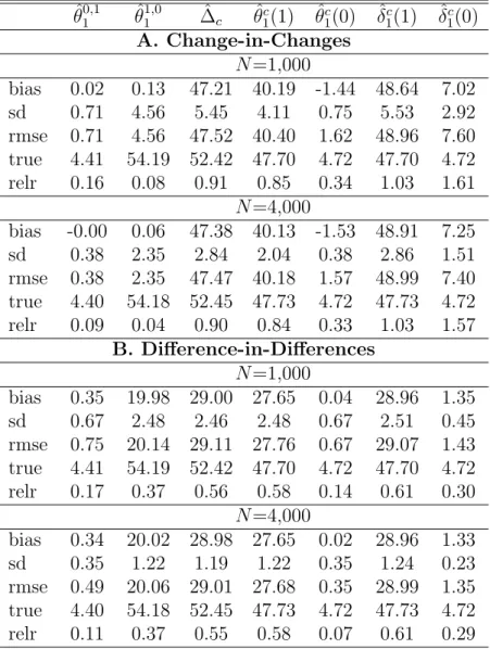
Table 3: Nonlinear model with non-random treatment ˆ θ10,1 θˆ11,0 ∆ˆc θˆc1(1) θˆc1(0) δˆ1c(1) δˆc1(0) A. Change-in-Changes N =1,000 bias 0.02 0.13 47.21 40.19 -1.44 48.64 7.02 sd 0.71 4.56 5.45 4.11 0.75 5.53 2.92 rmse 0.71 4.56 47.52 40.40 1.62 48.96 7.60 true 4.41 54.19 52.42 47.70 4.72 47.70 4.72 relr 0.16 0.08 0.91 0.85 0.34 1.03 1.61 N =4,000 bias -0.00 0.06 47.38 40.13 -1.53 48.91 7.25 sd 0.38 2.35 2.84 2.04 0.38 2.86 1.51 rmse 0.38 2.35 47.47 40.18 1.57 48.99 7.40 true 4.40 54.18 52.45 47.73 4.72 47.73 4.72 relr 0.09 0.04 0.90 0.84 0.33 1.03 1.57 B. Difference-in-Differences N =1,000 bias 0.35 19.98 29.00 27.65 0.04 28.96 1.35 sd 0.67 2.48 2.46 2.48 0.67 2.51 0.45 rmse 0.75 20.14 29.11 27.76 0.67 29.07 1.43 true 4.41 54.19 52.42 47.70 4.72 47.70 4.72 relr 0.17 0.37 0.56 0.58 0.14 0.61 0.30 N =4,000 bias 0.34 20.02 28.98 27.65 0.02 28.96 1.33 sd 0.35 1.22 1.19 1.22 0.35 1.24 0.23 rmse 0.49 20.06 29.01 27.68 0.35 28.99 1.35 true 4.40 54.18 52.45 47.73 4.72 47.73 4.72 relr 0.11 0.37 0.55 0.58 0.07 0.61 0.29
Note: ‘bias’, ‘sd’, and ‘rmse’ provide the bias, standard deviation, and root mean squared error of the respective estimator. ‘true’ and ‘relr’ are the respective true effect as well as the root mean squared error relative to the true effect.
In our final simulation design, we maintain the exponential outcome model but assume D to be selective w.r.t. U rather than random. To this end, the treatment model in (4) is replaced by D = I{U + Q > 0}, with the independent variable Q ∼ N (0, 1) being an unobserved term. Under this violation of Assumption 7,
complier shares and effects are no longer identified, which is confirmed by the sim-ulation results presented in Table3. The bias in the change-in-changes based total, direct, and indirect effects on compliers do not vanish as the sample size increases. Furthermore, under non-random assignment of D (while maintaining monotonicity of M in D), the never-takers’ and always-takers’ respective distributions of U dif-fer across treatment. Therefore, average direct effects among the total of never or always-takers, respectively, are not identified. Yet, θ1,01 , which is still identified by the same estimator as before, yields the direct effect among never-takers with D = 1 (as defiers do not exist). Likewise, θ0,11 corresponds to the direct effect on always-takers with D = 0. Indeed, the results in Table 3suggest that both parameters are consistently estimated with the change-in-changes model (Panel A.).
5
Application
Our empirical application is based on the JOBS II data byVinokur and Price(1999). JOBS II was a randomized job training intervention in the US, designed to anal-yse the impact of job training on labour market and mental health outcomes, see
Vinokur, Price, and Schul (1995). It was a modified version of the earlier JOBS programme, which had been found to improve labour market outcomes such as job satisfaction, motivation, earnings, and job stability, seeCaplan, Vinokur, Price, and van Ryn(1989) andVinokur, van Ryn, Gramlich, and Price(1991), as well as mental health, seeVinokur, Price, and Caplan (1991). According to the results ofVinokur, Price, and Schul(1995), the JOBS II programme increased reemployment rates and improved mental health outcomes, especially for participants having an elevated risk of depression. The JOBS interventions had an important impact in the academic literature (see e.g. Wanberg, 2012, Liu, Huang, and Wang, 2014) and the method-ology was implemented in field experiments in Finland (Vuori, Silvonen, Vinokur, and Price, 2002, Vuori and Silvonen, 2005) and the Netherlands (Brenninkmeijer and Blonk,2011), suggesting positive effects on labour market integration in either
The JOBS II intervention was conducted in south-eastern Michigan, where 2,464 job seekers were eligible to participate in a randomized field experiment, seeVinokur and Price(1999). In a baseline period prior to programme assignment, individuals responded to a screening questionnaire that collected pre-treatment information on mental health. Based on the latter, individuals were classified as having either a high or low depression risk and those with a high risk were oversampled before the training was randomly assigned.1 The job training consisted of five 4-hours seminars
conducted in morning sessions during one week between March 1 and August 7, 1991. Members of the treatment group who participated in at least four of the five sessions received USD 20. Each of the standardized training sessions consisted, among other aspects, of the learning and practicing of job search and problem-solving skills.2 The control group received a booklet with information on job search methods (Vinokur, Price, and Schul, 1995, p. 44-49).
We analyse the impact of job training on mental health, namely symptoms of depression 6 months after training participation. The health outcome (Y ) is based on a 11-items index of depression symptoms of the Hopkins Symptom Checklist. For example, respondents were asked how much they were bothered by symptoms such as crying easily, feeling lonely, feeling blue, feeling hopeless, having thoughts of ending their lives, or experiencing a loss of sexual interest. The questions were coded on a 5-point scale, going from ‘not at all’ (1) to ‘extremely’ (5), and summarized in a depression variable that consists of the average across all questions.
One-sided non-compliance with the random assignment is a major issue in JOBS 1In the JOBS II intervention, randomization was followed by yet another questionnaire sent out two
weeks before the actual job training, seeVinokur, Price, and Schul (1995), which also provided information on whether an individual had been assigned the training. Consequently, the data collected in that questionnaire must be considered post-treatment as they could be affected by learning the assignment. Therefore, we rely on the earlier screening data as the relevant pre-treatment period prior to random programme assignment.
2When compared to the earlier JOBS programme (Caplan, Vinokur, Price, and van Ryn, 1989),
the job training sessions of JOBS II focused more strongly on building a sense of mastery, personal control and self- efficacy in job search. Previous research had suggested that an increase in this sense of mastery, control and self-efficacy improved observed effort in job search behaviour (Eden and Aviram,1993). Results in Marshall and Lang(1990) suggest that mastery is a strong predictor of depression symptoms among women. For a detailed discussion of the literature, the exact sampling process, the training programme, and further aspects, seeVinokur, Price, and Schul(1995).
II. While the study design rules out always-takers because members of the control group did not have access to the job training programme, 45% of those assigned to training in our data did not participate and are therefore never-takers, the remaining 55% are compliers. In order to avoid selection bias w.r.t actual participation, the original JOBS II study by Vinokur, Price, and Schul (1995) analysed the total effect of the policy (i.e. the intention-to-treat effect), including those who, despite receiving an offer to participate, did not take part in the job training. In contrast, we use our methodology to separate the direct effect of mere training assignment, which is our treatment D, from the indirect effect operating through actual training participation, which is our mediator M , among compliers.3 We also consider the direct effect on never-takers, which likely differs from that on the compliers. While being offered (or not offered) the job training might affect compliers’ mental health by inducing motivation/enthusiasm (or discouragement), it may not have the same effect among never-takers, who do not attend such seminars whatsoever.
More concisely, we base identification on Theorem 3a with Assumption 4a for the average direct effect on never-takers, θn
1, on Theorem 3b with Assumption 4 for the direct effect on compliers under d = 0, θ1c(0), and Theorem 5 with Assumptions 4b and 6a for the indirect effect on compliers under d = 1, δ1c(1). None of these approaches requires the presence of always-takers in the sample. We also note that if random assignment operated through other mechanisms than actual participation in any of the subpopulations as it may appear reasonable in the context of mental health outcomes, this would violate the exclusion restriction when using assignment as instrumental variable for actual participation in a two stage least squares regression. Given that our identifying assumptions hold, our approach can therefore be used to statistically test the exclusion restriction.
Our evaluation sample consists of a total of 3,360 observations in the pre-treatment and post-mediator periods with non-missing information for D, M , and Y . It is an 3Imai, Keele, and Tingley(2010) analyse Jobs II in a mediation context as well, but consider a
different mediator, namely job search self-efficacy, and a different identification strategy based on selection on observables.
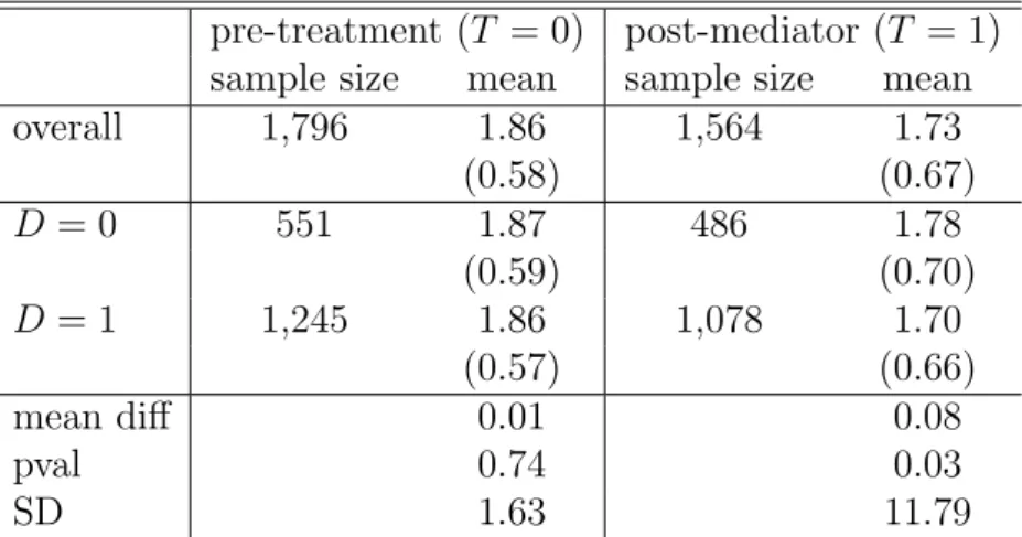
Table 4: Descriptive statistics on outcomes in pre- and post-mediator periods pre-treatment (T = 0) post-mediator (T = 1)
sample size mean sample size mean
overall 1,796 1.86 1,564 1.73 (0.58) (0.67) D = 0 551 1.87 486 1.78 (0.59) (0.70) D = 1 1,245 1.86 1,078 1.70 (0.57) (0.66) mean diff 0.01 0.08 pval 0.74 0.03 SD 1.63 11.79
Note: Standard deviations are in parentheses. ‘mean diff’, ‘pval’, and ‘SD’ are the mean difference, its p-value, and the standardized difference, respectively.
unbalanced panel due to attrition of roughly 13% of the initial respondents between the two periods. Table 4 provides summary statistics for the outcome in the total sample as well as by treatment group over time. We verify whether randomiza-tion was successful by comparing the outcome means of the treatment and control groups in the pre-treatment period (T = 0) just prior to the randomization of D. The small difference of 0.01 is not statistically significant according to a two sample t-test. Furthermore, the standardized difference test suggested by Rosenbaum and Rubin (1985) yields a value of just 1.68 and is thus far below 20, a threshold fre-quently chosen for indicating problematic imbalances across treatment groups. To test for potential attrition bias we also consider these statistics in the pre-treatment period exclusively among the panel cases that remain in the sample in the post-mediator period (not reported in Table 4). The p-value of the t-test amounts to 0.52 and the standardized difference of 3.5 is low such that attrition bias does not appear to be a concern. We therefore do not find statistical evidence for a violation of the random assignment of D in our sample. Table4also reports the mean differ-ence in outcomes in the post-mediator period (T = 1) 6 months after participation, which is an estimate for the total (or intention-to-treat) effect of D. The difference of 0.08 is statistically significant at the 5% level.
Table 5: Empirical results for Jobs II
Changes-in-Changes Difference-in-Differences Type shares ˆ θn 1 ∆ˆc θˆ1c(0) ˆδ1c(1) θˆ1n ∆ˆc θˆc1(0) δˆ1c(1) p(n)ˆ p(c)ˆ est -0.04 -0.11 0.06 -0.17 -0.03 -0.12 -0.06 -0.06 0.45 0.55 se 0.05 0.06 0.05 0.08 0.05 0.06 0.05 0.07 0.01 0.01 pval 0.40 0.06 0.26 0.04 0.52 0.03 0.21 0.43 0.00 0.00
Note: ‘est’, ‘se’, and ‘pval’ provide the effect estimate, standard error, and p-value of the respective estimator. ˆp(n) and ˆp(c) are the estimated never-taker and complier shares. Standard errors are based on cluster bootstrapping the effects 1999 times where clustering is on the respondent level.
strategy ofDeuchert, Huber, and Schelker(2017) when (linearly) controlling for the gender of respondents in either case. Standard errors rely on cluster bootstrapping the direct and indirect effects 1999 times, where clustering is on the respondent level. The CiC and DiD estimates of the direct effects on never-takers, ˆθn1(0), as well as on compliers, ˆθc1(0), are not statistically significant at conventional levels. Hence, we do not find statistical evidence for a direct effect of the mere assignment into the training programme on the depression outcome, which would point to a violation of the exclusion restriction when using assignment as instrument for par-ticipation. In contrast, we find for both CiC and DiD negative total effects among compliers ˆ∆c that are statistically significant at least at the 10% level. In the case of CiC, also the negative indirect effect among compliers, ˆδ1c(1), is significant at the 5% level, while this is not in the case for DiD. By and large, our results point to a moderately negative treatment effect on depressive symptoms through actual pro-gramme participation, rather than through other (i.e. direct) mechanisms. The CiC estimates ˆδc
1(1) and ˆ∆c are in fact rather similar to the result of a two stage least squares regression relying on the exclusion restriction by using D as instrument for M . The latter approach yields a local average treatment effect on compliers in the post-mediator period of -0.14 with a heteroskedasticity-robust standard error of 0.07 (significant at the 5% level).
6
Conclusion
We proposed a novel identification strategy for causal mediation analysis with re-peated cross sections or panel data based on changes-in-changes (CiC) assumptions that are related but yet different to Athey and Imbens (2006) considering total treatment effects. Strict monotonicity of outcomes in unobserved heterogeneity and distributional time invariance of the latter within groups defined on treatment and mediator states are key assumptions for identifying direct effects within these groups. Additionally assuming random treatment assignment and weak monotonicity of the mediator in the treatment permits identifying direct effects on never-takers and always-takers as well as total, direct, and indirect effects on compliers. We also provided a brief simulation study and an empirical application to the Jobs II pro-gramme.
References
Albert, J. M., and S. Nelson (2011): “Generalized causal mediation analysis,” Biometrics, 67, 1028–1038.
Angrist, J. D., G. W. Imbens, and D. B. Rubin (1996): “Identification of Causal Effects Using Instrumental Variables,” Journal of the American Statistical Association, 91, 444–472.
Athey, S., and G. W. Imbens (2006): “Identification and Inference in Nonlinear Difference-In-Difference Models,” Econometrica, 74, 431–497.
Baron, R. M.,andD. A. Kenny (1986): “The Moderator-Mediator Variable Dis-tinction in Social Psychological Research: Conceptual, Strategic, and Statistical Considerations,” Journal of Personality and Social Psychology, 51, 1173–1182.
Bellani, L., and M. Bia (2018): “The long-run effect of childhood poverty and the mediating role of education,” Journal of the Royal Statistical Society: Series A, 182, 37–68.
Bijwaard, G. E., and A. M. Jones (2019): “An IPW estimator for mediation effects in hazard models: with an application to schooling, cognitive ability and mortality,” Empirical Economics, 57, 129–175.
Brenninkmeijer, V.,and R. W. Blonk (2011): “The effectiveness of the JOBS program among the long-term unemployed: a randomized experiment in the Netherlands,” Health Promotion International, 27, 220–229.
Brunello, G., M. Fort, N. Schneeweis, and R. Winter-Ebmer (2016): “The Causal Effect of Education on Health: What is the Role of Health
Behav-iors?,” Health Economics, 25, 314–336.
Callaway, B. (2016): “Quantile Treatment Effects in R: The qte Package,” working paper, Temple University, Philadelphia.
Caplan, R. D., A. D. Vinokur, R. H. Price, and M. van Ryn (1989): “Job seeking, reemployment, and mental health: A randomized field experiment in coping with job loss,” Journal of Applied Psychology, 74, 759–769.
Chaisemartin, C., and X. D’Haultfeuille (2018): “Fuzzy Differences-in-Differences,” Review of Economic Studies, 85, 999–1028.
Chen, S. H., Y. C. Chen, and J. T. Liu (2017): “The impact of family compo-sition on educational achievement,” Journal of Human Resources, 0915-7401R1.
Cochran, W. G. (1957): “Analysis of Covariance: Its Nature and Uses,” Biomet-rics, 13, 261–281.
Conti, G., J. J. Heckman,andR. Pinto (2016): “The Effects of Two Influential Early Childhood Interventions on Health and Healthy Behaviour,” The Economic Journal, 126, F28–F65.
Deuchert, E., M. Huber, and M. Schelker (2017): “Direct and indirect ef-fects based on difference-in-differences with an application to political preferences
following the Vietnam draft lottery,” forthcoming in the Journal of Business & Economic Statistics.
Doerr, A., and A. Strittmatter (2019): “Identifying causal channels of policy reforms with multiple treatments and different types of selection,” working paper, University of St. Gallen.
Eden, D., and A. Aviram (1993): “Self-efficacy training to speed reemployment: Helping people to help themselves,” Journal of Applied Psychology, 78, 352–360.
Flores, C. A., and A. Flores-Lagunes (2009): “Identification and Estimation of Causal Mechanisms and Net Effects of a Treatment under Unconfoundedness,” IZA Discussion Paper No. 4237.
Frangakis, C., and D. Rubin (2002): “Principal Stratification in Causal Infer-ence,” Biometrics, 58, 21–29.
Fr¨olich, M., and M. Huber (2017): “Direct and Indirect Treatment Effects – Causal Chains and Mediation Analysis with Instrumental Variables,” Journal of the Royal Statistical Society: Series B, 79, 1645–1666.
Heckman, J., R. Pinto, and P. Savelyev (2013): “Understanding the Mech-anisms Through Which an Influential Early Childhood Program Boosted Adult Outcomes,” American Economic Review, 103, 2052–2086.
Hong, G. (2010): “Ratio of mediator probability weighting for estimating natural direct and indirect effects,” in Proceedings of the American Statistical Association, Biometrics Section, p. 2401–2415. Alexandria, VA: American Statistical Associa-tion.
Huber, M. (2014): “Identifying causal mechanisms (primarily) based on inverse probability weighting,” Journal of Applied Econometrics, 29, 920–943.
Huber, M. (2015): “Causal pitfalls in the decomposition of wage gaps,” Journal of Business and Economic Statistics, 33, 179–191.
Huber, M., M. Lechner, and G. Mellace (2017): “Why Do Tougher Case-workers Increase Employment? The Role of Program Assignment as a Causal Mechanism,” The Review of Economics and Statistics, 99, 180–183.
Huber, M., M. Lechner, and A. Strittmatter (2018): “Direct and indirect effects of training vouchers for the unemployed,” Journal of the Royal Statistical Society: Series A (Statistics in Society), 181, 441–463.
Imai, K., L. Keele, and D. Tingley (2010): “A General Approach to Causal Mediation Analysis,” Psychological Methods, 15, 309–334.
Imai, K., L. Keele, and T. Yamamoto (2010): “Identification, Inference and Sensitivity Analysis for Causal Mediation Effects,” Statistical Science, 25, 51–71.
Imai, K., and T. Yamamoto (2013): “Identification and Sensitivity Analysis for Multiple Causal Mechanisms: Revisiting Evidence from Framing Experiments,” Political Analysis, 21, 141–171.
Imbens, G. W., and J. Angrist (1994): “Identification and Estimation of Local Average Treatment Effects,” Econometrica, 62, 467–475.
Judd, C. M., andD. A. Kenny (1981): “Process Analysis: Estimating Mediation in Treatment Evaluations,” Evaluation Review, 5, 602–619.
Juhn, C., K. M. Murphy,and B. Pierce (1991): “Accounting for the Slowdown in Black-White Wage Convergencee,” in Workers and their Wages: Changing Pat-terns in the United States, ed. by M. H. Kosters, pp. 107–143. American Enterprise Insitute, Washigton.
Keele, L., D. Tingley, and T. Yamamoto (2015): “Identifying mechanisms behind policy interventions via causal mediation analysis,” Journal of Policy Anal-ysis and Management, 34, 937–963.
Inter-Manski, C. F. (1988): Analog Estimation Methods in Econometrics. Chapman & Hall, New York.
Marshall, G. N., and E. L. Lang (1990): “Optimism, self-mastery, and symp-toms of depression in women professionals,” Journal of Personality and Social Psychology, 59, 132–139.
Melly, B., and G. Santangelo (2015): “The Changes-in-Changes Model with Covariates,” Working Paper.
Pearl, J. (2001): “Direct and indirect effects,” in Proceedings of the Seventeenth Conference on Uncertainty in Artificial Intelligence, pp. 411–420, San Francisco. Morgan Kaufman.
Petersen, M. L., S. E. Sinisi, and M. J. van der Laan (2006): “Estimation of Direct Causal Effects,” Epidemiology, 17, 276–284.
Powdthavee, N., W. N. Lekfuangfu, and M. Wooden (2013): “The
Marginal Income Effect of Education on Happiness: Estimating the Direct and Indirect Effects of Compulsory Schooling on Well-Being in Australia,” IZA Dis-cussion Paper No. 7365.
Robins, J. M. (2003): “Semantics of causal DAG models and the identification of direct and indirect effects,” in In Highly Structured Stochastic Systems, ed. by P. Green, N. Hjort, and S. Richardson, pp. 70–81, Oxford. Oxford University Press.
Robins, J. M., and S. Greenland (1992): “Identifiability and Exchangeability for Direct and Indirect Effects,” Epidemiology, 3, 143–155.
Rosenbaum, P. R.,andD. B. Rubin (1985): “Constructing a control group using multivariate matched sampling methods that incorporate the propensity score.,” The American Statistician, 39, 33–38.
Rubin, D. B. (1974): “Estimating the Causal Effect of Treatments in Randomized and Non-Randomized Studies,” Journal of Educational Psychology, 66, 688–701.
Rubin, D. B. (2004): “Direct and Indirect Causal Effects via Potential Outcomes,” Scandinavian Journal of Statistics, 31, 161–170.
Simonsen, M., and L. Skipper (2006): “The Costs of Motherhood: An Analysis Using Matching Estimators,” Journal of Applied Econometrics, 21, 919–934.
Strittmatter, A. (2019): “Heterogeneous Earnings Effects of the Job Corps by Gender Earnings: A Translated Quantile Approach,” forthcoming in Labour Eco-nomics.
Tchetgen Tchetgen, E. J., and I. Shpitser (2012): “Semiparametric the-ory for causal mediation analysis: Efficiency bounds, multiple robustness, and sensitivity analysis,” The Annals of Statistics, 40, 1816–1845.
VanderWeele, T. J. (2008): “Simple relations between principal stratification and direct and indirect effects,” Statistics & Probability Letters, 78, 2957–2962.
VanderWeele, T. J. (2009): “Marginal Structural Models for the Estimation of Direct and Indirect Effects,” Epidemiology, 20, 18–26.
VanderWeele, T. J. (2012): “Comments: Should Principal Stratification Be Used to Study Mediational Processes?,” Journal of Research on Educational Effective-ness, 5, 245–249.
Vansteelandt, S., M. Bekaert,and T. Lange (2012): “Imputation Strategies for the Estimation of Natural Direct and Indirect Effects,” Epidemiologic Methods, 1, 129–158.
Vinokur, A. D., and R. H. Price (1999): “Jobs II Preventive Intervention for Unemployed Job Seekers, 1991-1993,” Inter-university Consortium for Political and Social Research.
Vinokur, A. D., R. H. Price, and R. D. Caplan (1991): “From field ex-periments to program implementation: Assessing the potential outcomes of an experimental intervention program for unemployed persons,” American Journal of Community Psychology, 19, 543–562.
Vinokur, A. D., R. H. Price, and Y. Schul (1995): “Impact of the JOBS Intervention on Unemployed Workers Varying in Risk for Depression,” American Journal of Community Psychology, 23, 39–74.
Vinokur, A. D., M. van Ryn, E. M. Gramlich, and R. H. Price (1991): “From field experiments to program implementation: Assessing the potential out-comes of an experimental intervention program for unemployed persons,” Journal of Applied Psychology, 76, 213–219.
Vuori, J., and J. Silvonen (2005): “The benefits of a preventive job search program on re-employment and mental health at 2-year follow-up,” Journal of Occupational and Organizational Psychology, 78, 43–52.
Vuori, J., J. Silvonen, A. D. Vinokur,andR. H. Price (2002): “The Ty¨oh¨on Job Search Program in Finland: Benefits for the Unemployed With Risk of De-pression or Discouragement,” Journal of Occupational Health Psychology, 7, 5–19.
Wanberg, C. R. (2012): “The Individual Experience of Unemployment,” Annual Review of Psychology, 63, 369–396.
W¨uthrich, K. (2019): “A comparison of two quantile models with endogeneity,” forthcoming in Journal of Business and Economic Statistics.
Appendices
A
Proof of Theorem 1
A.1
Average direct effect under d = 1 conditional on D = 1
and M(1) = 0
In the following, we prove that θ11,0(1) = E[Y1(1, 0) − Y1(0, 0)|D = 1, Mi(1) = 0] = E[Y1 − Q00(Y0)|D = 1, M = 0]. Using the observational rule, we obtain E[Y1(1, 0)|D = 1, M (1) = 0] = E[Y1|D = 1, M = 0]. Accordingly, we have to show that E[Y1(0, 0)|D = 1, M (1) = 0] = E[Q00(Y0)|D = 1, M = 0] to finish the proof.
Denote the inverse of h(d, m, t, u) by h−1(d, m, t; y), which exists because of the strict monotonicity required in Assumption 1. Under Assumptions 1 and 3a, the conditional potential outcome distribution function equals
FYt(d,0)|D=1,M =0(y) A1 = Pr(h(d, m, t, U ) ≤ y|D = 1, M = 0, T = t), = Pr(U ≤ h−1(d, m, t; y)|D = 1, M = 0, T = t), A3a = Pr(U ≤ h−1(d, m, t; y)|D = 1, M = 0), = FU |10(h−1(d, m, t; y)), (A.1)
for d, d0 ∈ {0, 1}. We use these quantities in the following. First, evaluating FY1(0,0)|D=1,M =0(y) at h(0, 0, 1, u) gives
FY1(0,0)|D=1,M =0(h(0, 0, 1, u)) = FU |10(h
−1
(0, 0, 1; h(0, 0, 1, u))) = FU |10(u).
Applying FY−1
1(0,0)|D=1,M =0(q) to both sides, we have
h(0, 0, 1, u) = FY−1
Second, for FY0(0,0)|D=1,M =0(y) we have
FU |D=1,M =0−1 (FY0(0,0)|D=1,M =0(y)) = h
−1
(0, 0, 0; y). (A.3)
Combining (A.2) and (A.3) yields,
h(0, 0, 1, h−1(0, 0, 0; y)) = FY−1
1(0,0)|D=1,M =0◦ FY0(0,0)|D=1,M =0(y). (A.4)
Note that h(0, 0, 1, h−1(0, 0, 0; y)) maps the period 1 (potential) outcome of an in-dividual with the outcome y in period 0 under non-treatment without the me-diator. Accordingly, E[FY−1
1(0,0)|D=1,M =0 ◦ FY0(0,0)|D=1,M =0(Y0)|D = 1, M = 0] =
E[Y1(0, 0)|D = 1, M = 0]. We can identify FY0(0,0)|D=1,M =0(y) under Assumption
2, but we cannot identify FY1(0,0)|D=1,M =0(y). However, we show in the
follow-ing that we can identify the overall quantile-quantile transform FY−1
1(0,0)|D=1,M =0 ◦
FY0(0,0)|D=1,M =0(y) under the additional Assumption 3b.
Under Assumptions 1 and 3b, the conditional potential outcome distribution function equals FYt(d,0)|D=0,M =0(y) A1 = Pr(h(d, m, t, U ) ≤ y|D = 0, M = 0, T = t), = Pr(U ≤ h−1(d, m, t; y)|D = 0, M = 0, T = t), A3b = Pr(U ≤ h−1(d, m, t; y)|D = 0, M = 0), = FU |00(h−1(d, m, t; y)), (A.5)
for d, d0 ∈ {0, 1}. We repeat similar steps as above. First, evaluating FY1(0,0)|D=0,M =0(y)
at h(0, 0, 1, u) gives
FY1(0,0)D=0,M =0(h(0, 0, 1, u)) = FU |00(h
−1
(0, 0, 1; h(0, 0, 1, u))) = FU |00(u).
Applying FY−1
1(0,0)|D=0,M =0(q) to both sides, we have
h(0, 0, 1, u) = FY−1
Second, for FY0(0,0)|D=0,M =0(y) we have
FU |00−1 (FY0(0,0)|D=0,M =0(y)) = h
−1
(0, 0, 0; y). (A.7)
Combining (A.6) and (A.7) yields,
h(0, 0, 1, h−1(0, 0, 0; y)) = FY−1
1(0,0)|D=0,M =0◦ FY0(0,0)|D=0,M =0(y). (A.8)
The left sides of (A.4) and (A.8) are equal. In contrast to (A.4), (A.8) con-tains only distributions that can be identified from observable data. In partic-ular, FYt(0,0)|D=0,M =0(y) = Pr(Yt(0, 0) ≤ y|D = 0, M = 0) = Pr(Yt ≤ y|D =
0, M = 0). Accordingly, we can identify FY−1
1(0,0)|D=1,M =0 ◦ FY0(0,0)|D=1,M =0(y) by
Q00(y) ≡ FY−1
1|D=0,M =0◦ FY0|D=0,M =0(y).
Parsing Y0 through Q00(·) in the treated group without mediator gives
E[Q00(Y0)|D = 1, M = 0] = E[FY−1 1|D=0,M =0◦ FY0|D=0,M =0(Y0)|D = 1, M = 0], = E[FY−1 1(0,0)|D=0,M =0◦ FY0(0,0)|D=0,M =0(Y0(1, 0))|D = 1, M = 0], A1,A3b = E[h(0, 0, 1, h−1(0, 0, 0; Y0(1, 0)))|D = 1, M = 0], A2 = E[h(0, 0, 1, h−1(0, 0, 0; Y0(0, 0)))|D = 1, M = 0], A1,A3a = E[FY−1 1(0,0)|D=1,M =0◦ FY0(0,0)|D=1,M =0(Y0(0, 0))|D = 1, M = 0], = E[Y1(0, 0)|D = 1, M = 0] = E[Y1(0, 0)|D = 1, M (1) = 0], (A.9)
A.2
Quantile direct effect under d = 1 conditional on D = 1
and M(1) = 0
In the following, we prove that
θ11,0(q, 1) = FY−1 1(1,0)|D=1,M (1)=0(q) − F −1 Y1(0,0)|D=1,M (1)=0(q), = FY−1 1|D=1,M =0(q) − F −1 Q00(Y0)|D=1,M =0(q).
For this purpose, we have to show that
FY1(1,0)|D=1,M (1)=0(y) = FY1|D=1,M =0(y) and (A.10)
FY1(0,0)|D=1,M (1)=0(y) = FQ00(Y0)|D=1,M =0(y), (A.11)
which is sufficient to show that the quantiles are also identified. We can show (A.10) using the observational rule FY1(1,0)|D=1,M (1)=0(y) = FY1|D=1,M =0(y) = E[1{Y1 ≤
y}|D = 1, M = 0], with 1{·} being the indicator function. Using (A.9), we obtain
FQ00(Y0)|D=1,M =0(y) = E[1{Q00(Y0) ≤ y}|D = 1, M = 0], = E[1{FY−1 1|D=0,M =0◦ FY0|D=0,M =0(Y0) ≤ y}|D = 1, M = 0], = E[1{Y1(0, 0) ≤ y}|D = 1, M = 0], = FY1(0,0)|D=1,M (1)=0(y), (A.12)
which proves (A.11).
A.3
Average direct effect under d = 0 conditional on D = 0
and M(0) = 0
In the following, we show that θ0,01 (0) = E[Y1(1, 0) − Y1(0, 0)|D = 0, M (0) = 0] = E[Q10(Y0) − Y1|D = 0, M = 0]. Using the observational rule, we obtain