HAL Id: hal-00305217
https://hal.archives-ouvertes.fr/hal-00305217
Submitted on 1 Jan 2002HAL is a multi-disciplinary open access archive for the deposit and dissemination of sci-entific research documents, whether they are pub-lished or not. The documents may come from teaching and research institutions in France or abroad, or from public or private research centers.
L’archive ouverte pluridisciplinaire HAL, est destinée au dépôt et à la diffusion de documents scientifiques de niveau recherche, publiés ou non, émanant des établissements d’enseignement et de recherche français ou étrangers, des laboratoires publics ou privés.
improving real-time flood forecasting through
conceptual hydrological models
A. Brath, A. Montanari, E. Toth
To cite this version:
A. Brath, A. Montanari, E. Toth. Neural networks and non-parametric methods for improving real-time flood forecasting through conceptual hydrological models. Hydrology and Earth System Sciences Discussions, European Geosciences Union, 2002, 6 (4), pp.627-639. �hal-00305217�
Neural networks and non-parametric methods for improving
real-time flood forecasting through conceptual hydrological models
A. Brath, A. Montanari and E. Toth
DISTART, Università di Bologna, Viale Risorgimento 2, 40136 Bologna Email for corresponding author: [email protected]
Abstract
Time-series analysis techniques for improving the real-time flood forecasts issued by a deterministic lumped rainfall-runoff model are presented. Such techniques are applied for forecasting the short-term future rainfall to be used as real-time input in a rainfall-runoff model and for updating the discharge predictions provided by the model. Along with traditional linear stochastic models, both stationary (ARMA) and non-stationary (ARIMA), the application of non-linear time-series models is proposed such as Artificial Neural Networks (ANNs) and the ‘nearest-neighbours’ method, which is a non-parametric regression methodology. For both rainfall forecasting and discharge updating, the implementation of each time-series technique is investigated and the forecasting schemes which perform best are identified. The performances of the models are then compared and the improvement in the efficiency of the discharge forecasts achievable is demonstrated when i) short-term rainfall forecasting is performed, ii) the discharge is updated and iii) both rainfall forecasting and discharge updating are performed in cascade. The proposed techniques, especially those based on ANNs, allow a remarkable improvement in the discharge forecast, compared with the use of heuristic rainfall prediction approaches or the not-updated discharge forecasts given by the deterministic rainfall-runoff model alone.
Keywords: real-time flood forecasting, precipitation prediction, discharge updating, time-series analysis techniques
Introduction
All over the world, damage caused by flood and flash-flood events, in terms of both number of casualties and economic costs, increases steadily; it now ranks high among weather-related natural hazards. In Italy, the archive of the National Research Council’s AVI project (an acronym for Aree Vulnerate Italiane, Areas Affected by Landslides or Floods in Italy) of the National Group for the Prevention of Hydrogeological Disasters identified as many as 7178 flood events all over the country between 1918 and 1994, and 42.5% of the Italian municipalities were affected.
The development of data acquisition systems based on telemetry and satellite communication systems coupled with the increase in availability of computer resources enhances significantly the potential for providing real-time flood warning through flow forecasting methodologies, using current information on the river basin state. For small mountain catchments, where steep slopes shorten the
response time of the catchment to hours or even less (flash-floods), a prediction based solely on hydrometric measurements does not allow a lead-time long enough to take effective precautionary measures. Modelling of the rainfall-runoff transformation enables the hydrological forecast to be derived not only from past observations but also from forecasts of precipitation on the upper catchment. The rainfall-runoff modelling approaches generally used for real-time flood predictions in small and medium size basins are either black-box (or system-theoretic) or conceptual. Black-box models do not describe the hydrological processes occurring within the catchment, even in a simplified manner; on the other hand they can be formulated easily in an adaptive framework which has made their application extremely appealing in hydrological practice. Conceptual models, on the other hand, allow a description of large spatial and temporal scale conservation
and response laws that are in accordance with the observed large-scale behaviour of water in hydrological drainage basins, and hydrologists have now recognised that such models are more able to forecast under out-of-sample conditions, by comparison with black-box modelling (e.g. Brath and Rosso, 1993).
In the present work, the use of time-series analysis techniques for real-time improvement of the forecast provided by a conceptual deterministic rainfall-runoff model is presented.
A first attempt to improve discharge predictions is through the incorporation of a Quantitative Precipitation Forecasting (QPF) scheme. In fact, a discharge forecast based solely on rainfall observed up to the forecast time (and this framework is often implicit in operational flood forecasting practice) tacitly implies a prediction of no more rain and such a prediction is the worst possible in the course of a severe storm (Krzysztofowicz, 1995). Obtaining a reliable QPF, especially at a temporal and spatial resolution compatible with hydrological forecasting needs, is extremely difficult and great uncertainties still affect the performance of physically-based rainfall prediction models (Brath, 1999). In addition, the rainfall generation process is a very complex dynamic system, involving many interconnected control variables that have to be monitored at a very fine scale. A considerable amount of high quality data on a fine temporal and spatial grid would be needed for accurate deterministic rainfall forecasts; such information is rarely available. A possible alternative is to perform the short-term precipitation forecasts by means of univariate time-series analysis techniques (Brath et al., 1988; Burlando et al., 1993), thus allowing quick forecasts with the requirement of only a moderate amount of data of the current event. An additional advantage is that a model generating forecasts in a format suitable for direct input to a hydrological model, rather than requiring significant human and/or computer intervention to convert it to a hydrologically useful format, would be extremely useful in a real-time framework. Even if rainfall time-series are generally characterised by very low persistence in time, the driving force for most flash floods is heavy rain that persists over an area for a few hours. Maddox (1979) states that flash floods are associated with convective storms of a quasi-stationary nature, characterised by a focusing over a certain area (Georgakakos, 1986). In Mediterranean mountainous regions, too, the flooding risk becomes actual when the storm area remains nearly stationary for several hours. A typical catastrophic flood in the Mediterranean region is the consequence of outlying storms characterised by low variability of rainfall intensity in time and space (Rossi and Siccardi, 1988). In addition, if rainfall depths are averaged over the catchment before the
time-series processing, the efficiency of the rainfall forecasts is improved, compared to the forecasts issued for each one of the gauges separately before averaging the results, because of the greater variability of point precipitation rates (Burlando et al., 1993; Georgakakos and Hudlow, 1984). Hence, potentially dangerous storm events are characterised by a higher persistence in time in comparison with more frequent events so that time-series analyses exploiting such persistence seem to be adequate for the prediction of spatially averaged extreme rainfall intensities at an hourly time scale. In addition to input uncertainty, the forecasts are subject to uncertainties in both model structure and parameter values. The uncertainty introduced by the sources mentioned above may result in biased discharge forecasts, as shown by the difference between the simulated hydrograph and that actually measured up to the forecast time. A considerable degree of persistence was highlighted in the analysis of the errors of the discharge simulations generated in the present study; the plot of the sample autocorrelation function of the discharge error series (Fig. 1), suggests that coupling a deterministic rainfall-runoff model with a parallel simulation error-forecasting model, based on the latest error observations may improve the forecast. Output updating procedures are computationally simple and well established in operational hydrological practice (Moore, 1983) and their key advantage is the simplicity of application in a totally automated way to any rainfall-runoff model, no matter how complicated, without any need to alter its structure and physical meaning, or its operational implementation.
The paper describes the coupling of a deterministic rainfall-runoff model with univariate time-series analysis techniques used both for forecasting the future rainfall values to be provided as input to the hydrological model and for updating the discharges issued by the model. A real-world case study is developed to assess the improvement in discharge forecasts using linear stochastic processes, Artificial Neural Networks and the non-parametric nearest -neighbours method for rainfall forecasting and for discharge updating, applied separately and in cascade.
The investigation of non-linear time series analysis techniques (neural networks and nearest-neighbours method) is suggested by the observation that temporal variations in hydro-meteorological data often do not exhibit simple regularities and linear recurrence relations and their combination for describing the behaviour of such data is often inadequate. In addition, such techniques belong to the data-driven approaches, where no relationship between known parameters and observed values has to be hypothesised and no knowledge of the underlying process is needed.
The analysed time-series analysis
techniques
LINEAR MODELS
Linear stochastic processes are among the most widely used time-series techniques for modelling water resources. Frequently used are the AutoRegressive Integrated Moving Average models, denoted as ARIMA(p,d,q) models, where p and q are, respectively, the autoregressive and moving average orders and d is the order of differentiation, that is the number of differentiations operated on the original series to handle possible non-stationarities (Bras and Rodriguez-Iturbe, 1985). The differencing reduces the ARIMA to simple AutoRegressive Moving Average (ARMA) models, describing each observation of a time-series xt as a weighted sum of p previous data and the current as well as q previous values of a white noise process. Using the Box and Jenkins notation, the ARMA(p,q) model can be written symbolically in the compact form:
t t B x B) ( )η ( =Θ Φ (1)
where xt is the zero-mean time-series; ηt is a white noise,
i.e. an independent zero-mean random variable that is also not correlated with the past values of xt; Φand Θ are respectively the pth and qth order autoregressive and moving
average components and B is the backward shift operator, defined so that Bj x
t = xt-j.
Analogously, the ARIMA(p,d,q) model can be expressed as:
(2)
where d is the order of differentiation of the original data, that is the minimum non-negative integer necessary to obtain a stationary process by differencing the original series.
The method here applied for the estimation of the parameters is an approximation in the spectral domain of the Gaussian maximum likelihood function, which was first proposed by Whittle (1953). This approximation provides asymptotically consistent and normally distributed estimators of the unknown parameters for both Gaussian and non-Gaussian series. Beran (1994) gives a detailed description of this parameter estimation method.
In the following applications, it was preferred to perform no preliminary transformation of the data to make them as close to Gaussian as possible. In fact, Gaussianity of the data is not required for the forecast application of ARIMA models, since they provide the best linear prediction even in the non-Gaussian case (Brockwell and Davis, 1987).
For rainfall prediction, the application of low-order ARIMA models was considered, following the modelling framework proposed by Brath et al. (1988) and Burlando et al. (1993). Such a choice is justified by the findings by Obeysekera et al. (1987), who proved that the correlation structures of certain point process models for rainfall modelling, both burst and cluster based (Rodriguez-Iturbe, 1986), are equivalent to the correlation structures of low-order ARMA models.
As far as discharge updating is concerned, almost all the updating approaches implemented both in the literature and in practice are based on linear stochastic processes, because they are easy to programme and do not require much computational effort (Moore 1983; Kachroo, 1992).
t t dx B B B)(1 ) ( )
η
( − =Θ Φ -0.1 0.0 0.1 0.2 0.3 0.4 0.5 0.6 0.7 0.8 0.9 1.0 0 5 10 15 20 Lag A u to c o rr el a tio n f u n ct ionConfidence bands of the zero value at the 95% significance level
Fig. 1. Plot of the sample autocorrelation function of the hourly discharge error series
NON-LINEAR TIME-SERIES ANALYSIS METHODS
AutoRegressive Moving Average models (ARMA and ARIMA) assume linear relationships among past and present values of the analysed variable, but temporal variations in real-world data often do not exhibit linear behaviour. Therefore, non-linear forecasters, namely Artificial Neural Networks (ANNs) and the nearest-neighbours methods are presented in this work.
Artificial Neural Networks (ANNs)
The predictive potentiality of Artificial Neural Networks (ANNs) is widely acknowledged and applications to a variety of problems, including simulation and forecasting of hydro-meteorological variables, have been presented in the literature. Most are dedicated to the prediction of river flows (at a time scale ranging from one year to one hour) both using only past flow observations (for example, Raman and Sunilkumar, 1995) and with exogenous input, that is, based on the knowledge of previous rainfall depths (and possibly other meteorological variables) along with past observed flows (amongst others, Hsu et al., 1995; Minns and Hall, 1996; Abrahart and Kneale, 1997; Shamseldin, 1997; Dawson and Wilby, 1998). The use of ANNs for rainfall forecasting and for simulation error forecasting has not been fully explored, as yet. In the rainfall forecasting field, extremely interesting applications were presented by French et al. (1992) and Kuligowski and Barros (1998). The present approach differs because the interest is here focused mainly on the hydrological use of rainfall forecasts: the scheme implemented provides a spatially averaged rainfall forecast for lead-times from one to six hours, directly usable as input to the rainfall-runoff lumped model; the only information used as input to the ANNs is the real past rainfall observations preceding each forecast instant.
Neural networks emulate the biological nervous system’s computational capacity by distributing computations to processing units called neurons, which are densely interconnected. The neurons are grouped in layers and adjacent layers are connected through synaptic links (weights). Three different layer types can be distinguished: an input layer, connecting the input information to the network (and not carrying out any computation), one or more hidden layers, acting as intermediate computational layers, and an output layer, producing the final output. In correspondence of a computational node J (Fig. 2), each one of the Nj entering values (IJi) is multiplied by a connection weight (wij). Such products are then all summed with a neuron-specific parameter, called bias (bj), used to scale the sum of products into a useful range. The computational node finally applies an activation function
(f) to the above sum to produce the node output (OJ). Weights (wij) and biases (bj) are determined by a non-linear optimisation procedure (training) that minimises a learning function expressing a closeness between observations and ANN outputs, in the present case the mean squared error. A set of observed input and output (called a target to be distinguished from the network final output) data pairs, the training data set, is processed repeatedly, changing the values of the parameters until they converge to values such that each input vector produces output values as close as possible to the desired target vectors. The final weights and biases of a successfully trained neural network represent its knowledge about the problem, knowledge that the network was not assumed to have a priori.
Unfortunately, no definitive established methodology exists to deal with the neural network modelling problem, because the optimal network architecture and characteristics are highly problem-dependent. In the present work, preliminary forecast analyses were performed on rainfall and simulation errors corresponding to a few storm events, to test different network architectures and properties: training algorithm, types of connection between the nodes, number of hidden layers and multistep ahead prediction schemes.
The popular and extensively tested BackPropagation (BP) training algorithm and several of its variants were examined. The BackPropagation algorithm is a supervised learning method in which the output error (difference between the network output and the target) is fed back through the network, using the gradient of the learning function to determine how to adjust the weights to minimise the error. To speed up the convergence rate, modifications to the basic steepest descent algorithm have been proposed recently, often borrowed from optimisation theory, like the Levenberg-Marquardt algorithm, a quasi-Newton method that proved to be the quickest and was less easily trapped in
bj + =
∑
= j i N i ijIJ b w f OJ J 1IJ
1IJ
2IJ
Nj j i N i ijIJ
b
w
J+
∑
=1w
1jw
2jw
Njj….
local minima among the algorithms tested; it was, therefore, chosen for the modelling applications in the present work. The possibility of different feedforward and feedback connections between the nodes was considered, leading to the choice of a classic multi-layer feedforward network (where only feedforward connections to adjacent layers are allowed, so that the information flows in only one direction, from the input through the hidden up to the output layer), because the addition of other types of connections between the layers (feedback and cascade-forward) required longer training times and more random initialisations of the parameters to provide substantially equivalent results.
The ‘Universal Approximation Theorem’ (Hornik et al., 1989) proves that only one layer of hidden units “suffices to approximate any function with finitely many discontinuities to arbitrary precision”, provided that the activation functions of the hidden units are non-linear and a sufficient number of hidden units is available. These results establish multilayer feedforward networks as a class of universal approximators. Provided that at least one hidden layer is present, there is no theory yet to tell how many hidden layers are needed but Zealand et al., (1999) noticed that the addition of hidden layers often fails to provide a noticeable improvement in the out-of-training forecasting application and a much longer training time is needed in comparison with the use of only one hidden layer. Networks formed by only one hidden layer were, therefore, tested.
Activation functions are needed for introducing non-linearity into the network and it is the non-non-linearity that makes multilayer networks so powerful. The exact form of the activation function is not critical, as long as it is bounded and it increases monotonically (Kuligowski and Barros, 1998). In the present work, one of the most widely used non-linear activation functions was chosen for the hidden nodes, that is a tan-sigmoidal unit
(3)
where I is the input to the node, that is the sum of the weighted products of outputs from previous nodes and of the bias of the node, and f(I) is the node output. For the output layer, instead, a linear transfer function was chosen. It was, in fact, preferable to choose an output activation function suited to the original distribution of targets, that in the present case are unbounded, rather than to force the data (with a standardisation or rescaling procedure) to conform to the output activation function.
For forecasting several time steps ahead (multistep ahead prediction), two methods have been considered. In the incremental or recursive multistep method, the network has only one output node, forecasting a single step ahead, and the network is applied recursively, using the previous predictions as inputs for the subsequent forecasts. Such an approach performs well for one-step ahead predictions but, since the forecast errors are propagated into subsequent forecasts, a strong deterioration is evidenced for increasing lead-times.
One of the major benefits of ANNs is the capability of a neural network to provide a multiple output when several nodes are included in the output layer. In the direct multistep method (Fig. 3), each output node represents one time step to be forecasted, so that the forecasts for all the lead-times are issued simultaneously. In this way, the longer lead-times are not penalised by error propagation; in fact, the overall performances indicate that such methods are more appropriate for multistep ahead predictions.
Finally, regarding the optimal number of nodes in the hidden layer, an ANN may suffer from either underfitting or overfitting. A network that is not sufficiently complex can fail to detect fully the signal in a complicated data set, resulting in an inability to generalise to problems never previously encountered (underfitting). On the other hand, a network with too large a number of hidden units may fit the training set exactly but it may learn spurious relationships peculiar to the training data (in essence, it fits also the noise)
( )
1 ) 1 ( 2 2 − + = − I e I f Xt Xt-1 Xt-NI+ 1 ... L ead-time = 1 Lead-time = 2 Lead-time = 3 Lead-time = 4 Lead-time = 5 L ead-time = 6 2 t Xˆ+ 3 t Xˆ + 4 t Xˆ+ 5 t Xˆ + 1 t Xˆ+ 6 t Xˆ+Fig.3. Direct multistep network: t is the forecast instant, Xt-1,…, Xt-NI+1 are the NI inputs, that is the observations (precipitation hourly depths or hourly discharge errors) preceding the forecast instant, Xt+1,…, Xt+6 are the outputs, that is the 1 to 6 hours ahead forecasts.
and become lacking in generalisation capability (overfitting). In consequence, the training performance generally improves as the number of hidden nodes increases, whereas the performance on an external validation set tends to deteriorate when the hidden nodes become too numerous. In addition, too large a network may take an unacceptably long time to be trained. There is really no way to establish the optimal dimensions of the hidden layer just from the number of outputs and training samples. Extensive trial-and-error tests for determining the most appropriate numbers of nodes will be described later.
The nearest-neighbours method (K-NN)
The nearest-neighbours method is a non-parametric method, as indicated by the absence of any parameterised analytical function of the input-output relationship, both a priori and a posteriori (that is, after a calibration or training phase). The characteristics of the most recent observations are, instead, used to guide the search for the approximation of future evolution through a locally fitted model. Yakowitz (1987) and Karlsson and Yakowitz(1987) extended the K-NN method, originally a pattern recognition procedure, to time-series and forecasting problems, constructing a robust theoretical base for the K-NN method and introducing it into the hydrological research world, where successful forecasting applications were developed (Galeati, 1990; Shamseldin and O’Connor, 1996; Todini, 2000).
In the context of univariate time-series forecasting, for each forecast instant t, a D-dimensional feature vector is defined as the vector of the D past observations of the variable x,
xD(t) = (x
t-D+1,…, xt), (4)
which the method assumes to be able to summarise statistically the entire past of the forecast instant t. Given the feature vector at instant t, xD(t), the set S
K,D of K past
nearest-neighbours of xD(t) may be identified, i.e. the K
D-dimensional vectors xD(t
j) belonging to a set of past
observations that minimise the Euclidean distance: (5) That is, to any D-ple that is not included in the K-dimensional set SK,D, corresponds to a distance from the feature vector that is larger than any of the distances between the feature vector and each one of the nearest-neighbours. The estimation of the values following the forecast instant t is then the sample average of the successors to the nearest-neighbours:
(6) where
It should here be noted that the nearest-neighbour prediction scheme is such that, as Eqn. (6) indicates, in no case can a value higher than the maximum historical rainfall depth be predicted and this may affect the generality of the method when it is used in forecasting extreme events.
Karlsson and Yakowitz (1987) proved that the K-NN predictor based on the feature vector is asymptotically optimal among all the predictors defined on the feature vector xD(t). That is, under fairly general circumstances,
convergence to the optimal predictor is assured as the historical data set increases.
Case study, rainfall-runoff model and
calibration approaches
The study catchment is the Sieve River basin, a tributary of the Arno River in Central Italy. The basin has a drainage area of 830 km2 and the time of concentration is about 10
hours. The data set consists of five years of hourly discharges at the closure section of Fornacina, hourly precipitation measured by 12 raingauges, to be spatially averaged, and temperature observations at four gauges (used, along with climatological data, for the estimation of potential evapotranspiration needed in the continuous rainfall-runoff simulation).
The deterministic model chosen in the present work to simulate the rainfall-runoff transformation is a conceptual lumped and continuously-simulated model called A Distributed Model (ADM), (Franchini, 1996), based on the concept of probability-distributed soil moisture storage capacity. The catchment is assumed composed of an infinite number of elementary areas (each one with a different soil moisture content and a different soil moisture capacity) and the proportion of elementary areas that are saturated is described by a distribution function: the total surface runoff is the spatial integral of the infinitesimal contribution deriving from the saturated elementary areas. The model is divided into two main blocks: the first represents the water balance at soil level, while the second represents the transfer of runoff production at the basin outlet. The soil, in turn, is divided into two zones: the upper zone produces surface and subsurface runoff, having as inputs precipitation and potential evapotranspiration, while the lower zone (whose input from the first one is percolation) produces base runoff.
2 1 2 1 D 1 1 D D()-x ( ) || ( ( ) ) x || −+ = −+ − =
∑
t i i i t j x xj t t , 1 ˆ 1∑
= + + = K j L t L t K xj x(
xtj D xtj xtj)
tj SK,D D 1 1,..., − , =x ( )∈ + −The transfer of these components to the outlet section takes place in two distinct stages: the first represents the flow along the hillslopes towards the channel network; the second is the flow along the channel network towards the basin outlet. The 11 parameters of the ADM model were calibrated off-line on the Sieve river basin with the Shuffled Complex Evolution (SCE-UA) global optimisation algorithm (Duan et al., 1992), which is both effective (consistently able to find the region of the global optimum) and efficient (not requiring too many objective function evaluations).
Because of the strong variability observable in the structures of the simulation error and of the precipitation series during the predominant dry or average conditions and during storm events, the analysis of the data was limited, both in calibration and validation phases, to the time intervals of storm events. In the observation period, a total of 84 storm events was identified and the corresponding precipitation and river discharge observations (for a total of 4580 hourly time steps) were collected. As the rainfall-runoff model is simulating continuously, the initial conditions preceding each forecast (and a forecast is issued in respect of all the instants of the events) are obtained from the model simulation using as input the observed rainfall data up to the forecast instant.
To estimate the parameters of the time-series analysis techniques, two different approaches were followed: sample calibration and adaptive calibration. In the split-sample calibration, the storm events were divided into two sets: a calibration (or training) set and a validation set, to test the performances of the calibrated model over out-of-sample occurrences. In the adaptive calibration, only the most recently observed values were supposed to be available for the calibration, so that the calibration of the time-series analysis model was implemented on-line, as soon as new observations became available. The nature of the nearest-neighbours method does not allow an adaptive calibration because the approach is based on the presence of an extended database where the search is made for the neighbours at the moment of forecast. It follows that only a split-sample calibration was implemented for the K-NN method.
Implementation of rainfall forecasting
The application of the above time-series techniques for issuing forecasts of spatially averaged rainfall depths and their use as input to the conceptual rainfall-runoff transformation model are here described briefly (full details may be found in Toth et al., 2000). Rainfall depth forecasts for lead-times from 1 to 6 hours were issued in respect of each hourly time step for all the events in the validation set and the performances of the resulting river forecasts wereanalysed and compared.
For each of the time-series methodologies (ARIMA models, ANN and K-NN method), the performances of various forecasting schemes, investigated through a trial-and-error process, were classified according to the RMSE (Root Mean Squared Error) of the hourly rainfall forecasts accumulated over the six steps ahead as compared to the 6-hour accumulated observed rainfall depths. The best performing implementation (optimal configuration) for each time-series analysis model was thus identified.
The rainfall forecasts described above were compared with those obtainable with simple heuristic forecasting approaches. The first one, often assumed implicitly when operating real-time rainfall-runoff models, hypothesises the future rainfall to be null (null rainfall approach). A second and a third predictive scheme extrapolate future values on the basis of the last measures, inferring some sort of persistence in the data: the persistent method sets the future rainfall intensity equal to the last measured value, for all the lead-times investigated (L=1 to 6 hours); the modified persistent method equates the intensity, for each given lead-time L, to the average intensity of the last L observations.
The methodologies implemented are compared in Tables 1a and 1b.
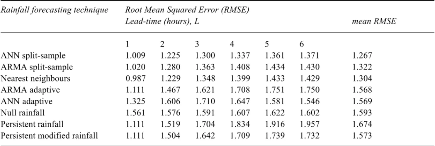
The three methods when calibrated with the split-sample procedure provided the smallest RMSE on the 6-hour accumulated rainfall, and especially good performances were achieved by non-linear models. Table 1 shows how ANN performed better than the nearest-neighbours method, which in turn was better than ARIMA models for the precipitation data available.
TRANSFORMATION OF RAINFALL FORECASTS IN DISCHARGE FORECASTS
The rainfall forecasts obtained in the previous section were then input to the rainfall-runoff model and the resulting discharge forecasts were evaluated using the coefficient of efficiency, E (Nash and Sutcliffe, 1970), compared to the hourly discharges obtained with the rainfall-runoff model using as inputs the actual future precipitation (true rainfall simulation). In this way, a comparison of the effects of the rainfall forecasting ability alone was allowed, unaffected by the uncertainties introduced in the rainfall-runoff transformation.
The coefficient of efficiency for each lead-time L is given by: , L = 1,....,6 (7)
∑
∑
− − − = + + + 2 2 ) ( ) ˆ ( 1 Q Q Q Q E L t L t L t LTable 1b. RMSE of the 1 to 6-hours ahead rainfall forecasts (obtained with the optimal configuration identified for each forecasting technique) issued for all the validation forecasts instants.
Rainfall forecasting technique Root Mean Squared Error (RMSE)
Lead-time (hours), L mean RMSE
1 2 3 4 5 6 ANN split-sample 1.009 1.225 1.300 1.337 1.361 1.371 1.267 ARMA split-sample 1.020 1.280 1.363 1.408 1.434 1.430 1.322 Nearest neighbours 0.987 1.229 1.348 1.399 1.433 1.429 1.304 ARMA adaptive 1.111 1.467 1.621 1.708 1.751 1.750 1.568 ANN adaptive 1.325 1.606 1.710 1.647 1.581 1.546 1.569 Null rainfall 1.561 1.576 1.591 1.607 1.622 1.602 1.593 Persistent rainfall 1.111 1.519 1.704 1.834 1.916 1.957 1.674
Persistent modified rainfall 1.111 1.504 1.642 1.709 1.739 1.732 1.573
Table 1a. RMSE of the sum of the 6-hours ahead rainfall forecasts issued for all the validation forecasts instants (that is, for all the time steps included in the events of the validation set).
Rainfall forecasting techniques Tested configurations Optimal configuration RMSE
ARIMA split-sample AutoRegressive order, p=1¸6, AutoRegressive order, p=1, Moving average order, q=0¸6, Moving average order, q=0,
Differentiation order, d=0,1, 2 Differentiation order, d=0 5.500 ARIMA adaptive AutoRegressive order, p=1¸2, AutoRegressive order, p=1,
Moving average order, q=0¸3, Moving average order, q=0,
Differentiation order, d=0,1, 2 Differentiation order, d=0 6.354
ANN split-sample Input nodes=2¸24 Input nodes=18
Hidden nodes=2¸8 Hidden nodes=2 5.083
ANN adaptive Input nodes=2¸5 Input nodes=3
Hidden nodes=2¸5 Hidden nodes=3 6.913
Nearest neighbours Number of neighbours, K=5¸100, Number of neighbours, K=70,
Feature vector dimension, D=2¸12 Feature vector dimension, D=2 5.343
Null rainfall 7.354
Persistent rainfall 8.063
Persistent modified rainfall 7.175
where Qˆt is the discharge at time t forecasted using as input the predicted rainfall values, Qt is the value of the corresponding true rainfall simulation discharge (known rainfall) and Q is the mean of the Qt series. The summations
are extended to all the issued forecasts, that is, to all the forecasts instants t belonging to all the validation events.
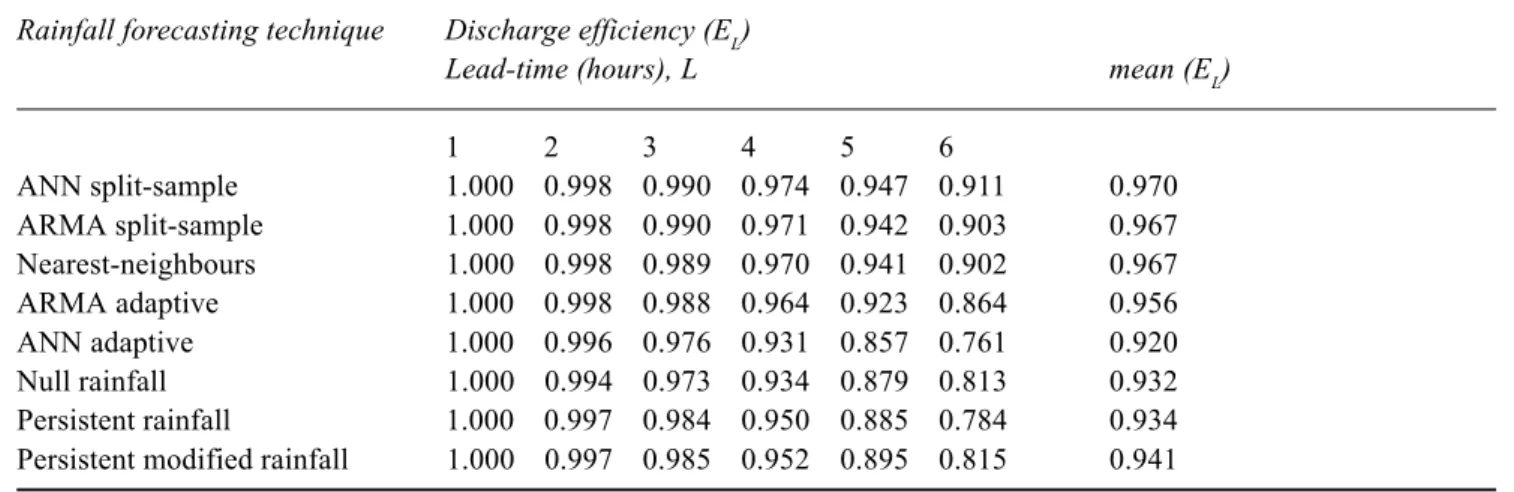
Table 2 shows how the hydrological processes governing the rainfall-runoff transformation tend to level out the discharge predictions corresponding to very short lead-times, because of the response time of the catchment. However,
the influence of the different rainfall forecasts on the discharges predicted for the longest lead-times is sizeable. The discharges simulated with the split-sampe calibrated ANNs provide, for all the lead-times, the highest efficiency values. The results of ARMA models with split-sample calibration and of the nearest-neighbours method are also satisfactory and allow a remarkable improvement in the discharge forecasts as compared to the heuristic rainfall forecasting approaches.
Implementation of discharge
updating
The objective of this section is to compare the performances of the time-series analysis techniques when applied for forecasting the simulation error on flood discharges, εt, i.e.
the difference between the observed discharges, Q0, and
those predicted by the conceptual model, Qs. The comparison
aims at identifying, from an operational point of view, the best approach for forecasting the future values of εt, in order
to update the future simulated discharges Qs. In this part of
the analysis, the Qs are the discharges issued by the
rainfall-runoff model when using as inputs the precipitation values that actually occurred. Such a working hypothesis implies a forecasting scenario in which future rainfall is known (‘perfect foresight’) for both calibration and verification sets, to be able to evaluate the improvement attainable with the discharge post-processing independently of the simulation errors induced by ignorance of future precipitation.
In the trial-and-error tests implemented for each time-series analysis technique, the efficiency coefficient, EL, of the discharges predicted with and without updating was computed for the lead-times, L, ranging from 1 to 6 hours. The average of EL over the six lead-times, E, was then used to identify the optimal configurations.
ARMA AND ARIMA MODELS FOR DISCHARGE UPDATING
In the split-sample calibration of ARIMA models, the maximum number of autoregressive and of moving average parameters was limited to three, and d varied from 0 to 2. The comparison of the efficiencies of the discharges updated with ARMA models (d=0) showed that a subgroup of
configurations allowed analogously good results (E=0.904 to 0.908). As a consequence, the ARMA(1,1) model was chosen for the overall comparison, as the most parsimonious among the better performing models (E=0.907). With the introduction of the differencing of the series, the performances deteriorated, the more so for increasing orders of differencing. The results corresponding to d=1 are sensibly worse than those allowed by the ARMA–type models with the same autoregressive and moving average orders (d=1: E=0.86 to 0.89), while the ARIMA models with differencing order d=2 are even worse (d=2: E=0.53 to 0.86).
In the adaptive calibration, the ARIMA orders tested were the same as those implemented in the split-sample calibration. The performance underwent, even more sharply than in the split-sample calibration, a strong deterioration for increasing order of differencing d, with a clear superiority of ARMA models over ARIMA models with the same autoregressive and moving average orders. Extremely parsimonious structures turned out to be the best performing ones, namely the ARMA(1,1) and the ARIMA(1,1,0) models. The linear models were calibrated initially on a number of observations, w, preceding the forecast instant initially set equal to 100 (that is on a moving window of 100 hours), following the indications of previous studies (Toth et al., 1999). It was of practical interest to test how performance changes with the length of the moving window. The results with the ARMA(1,1) model showed that the efficiency of the updating improved only moderately as w increased over 50 hourly observations. It may, therefore, be inferred that, in practice, good forecasting efficiency may be obtained with only a few observations from the current event (a couple of days)..
Table 2. Efficiency coefficients of the discharge forecasts corresponding to the different rainfall forecasts (issued for all the time steps belonging to the validation events) for varying lead-time (EL) and mean of the efficiency coefficients over the 6 lead-times (E).
Rainfall forecasting technique Discharge efficiency (EL)
Lead-time (hours), L mean (EL)
1 2 3 4 5 6 ANN split-sample 1.000 0.998 0.990 0.974 0.947 0.911 0.970 ARMA split-sample 1.000 0.998 0.990 0.971 0.942 0.903 0.967 Nearest-neighbours 1.000 0.998 0.989 0.970 0.941 0.902 0.967 ARMA adaptive 1.000 0.998 0.988 0.964 0.923 0.864 0.956 ANN adaptive 1.000 0.996 0.976 0.931 0.857 0.761 0.920 Null rainfall 1.000 0.994 0.973 0.934 0.879 0.813 0.932 Persistent rainfall 1.000 0.997 0.984 0.950 0.885 0.784 0.934
ANNS FOR DISCHARGE UPDATING
In the split-sample calibration, the test covered all the networks with a number of input nodes, NI, ranging from 2 to 24 hours and a number of hidden nodes, NH, ranging from two to eight. The networks with a medium input layer dimension (between 6 and 12) and a small number of hidden nodes gave the highest mean coefficients of efficiency. The network (8-2-6), corresponding to eight input nodes, two hidden nodes and six output nodes (lead-time = 6 hours) was identified as performing best (E=0.9114) but the performance gain in comparison to the networks with smaller input layers was extremely small. Given the modest improvement, a more parsimonious network was preferred and the ANN with four input nodes and two hidden nodes (E=0.9105) was chosen as the optimal configuration for the split-sample calibration application.
Simple network architectures were tested in the adaptive approach, with NI and NH ranging from two to four. The results indicated the most parsimonious structure (NI=2, NH=2) as the most efficient network (E=0.904).
NEAREST-NEIGHBOUR METHOD FOR DISCHARGE UPDATING
In regard to each dimension of the feature vector, D, ranging from 1 to 12, the number of nearest-neighbours, K, was gradually increased from 10 to 70.
When the number of neighbours increased from 10 to 20, there was a slight improvement but thereafter, the efficiency coefficient deteriorated. Small dimensions of the feature vector (D=2 to 4) provided the highest efficiencies of the updated discharges, so that the best performing implementation of the method resulted with K=20 neighbours and a dimension of the feature vector D=2 (E=0.899).
OVERALL COMPARISON OF DISCHARGE UPDATING
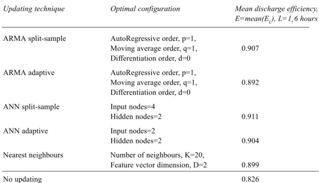
Table 3 shows the coefficients of efficiency (averaged over the lead-times) of the discharge forecasts updated with the best performing configurations identified in the trial-and-error tests for each time-series method and in Fig. 4 the performances of the various updating techniques in respect of increasing lead-times are illustrated.
The overall results highlight the relevant improvement allowed by all the methods analysed as compared to the not-updated discharge forecasts and show that the updating is worth implementing with all the time-series analysis techniques and over all the lead-times from one to six hours (with the only exception of the ARMA model adaptively calibrated for the longest lead-time).
The linear stochastic models provide very good results for small lead-times, especially for a lead-time of 1 hour, whereas for larger lead-times the performance of the ARMA
Table 3. Mean over the six lead-times (L=1¸6 hours) of the efficiency coefficients (EL) of the updated discharge forecasts (issued for all the time steps belonging to the validation events) for each updating time-series analysis technique.
Updating technique Optimal configuration Mean discharge efficiency,
E=mean(EL), L=1¸6 hours ARMA split-sample AutoRegressive order, p=1,
Moving average order, q=1, 0.907 Differentiation order, d=0
ARMA adaptive AutoRegressive order, p=1,
Moving average order, q=1, 0.892 Differentiation order, d=0
ANN split-sample Input nodes=4
Hidden nodes=2 0.911
ANN adaptive Input nodes=2
Hidden nodes=2 0.904
Nearest neighbours Number of neighbours, K=20,
Feature vector dimension, D=2 0.899
model adaptively calibrated deteriorates badly. This is to be expected as the AR(I)MA models use a recursive type scheme to perform the multi-step ahead forecasts and therefore tend to accumulate errors as the lead-time increases.
An extremely good performance is provided for longer lead-times by ANNs adaptively calibrated, but ANNs with split-sample calibration allow the greatest overall gain over not-updated discharges, for all the lead-times (Table 3).
Integrated implementation of rainfall
forecasting and discharge updating
Following the separate implementation of rainfall forecasting and discharge updating techniques, the performance of an integrated flood warning approach, operating with both the input prediction and the output correction modules, was analysed.Each model used for discharge updating was thus re-calibrated on the simulation errors resulting when using the rainfall predictions as input to the hydrological model, rather than assuming advance knowledge of future precipitation values. For both rainfall forecasting and discharge updating, the same time-series analysis technique (ARIMA models, ANNs or nearest-neighbours method) and the same calibration (split-sample or adaptive) were used, following the indications on the most appropriate modelling schemes obtained previously. 0.80 0.82 0.84 0.86 0.88 0.90 0.92 0.94 0.96 0.98 1.00 1 2 3 4 5 6 Lead-time (hours) Ef fi ci en cy ARMA split-sample ARMA adaptive ANN split-sample ANN adaptive Nearest neighbours No updating
Fig.4. Overall comparison of the efficiency coefficients for the updated discharges of the validation data set
corresponding to the best configurations for all the considered time-series methods
The results (Fig. 5) confirm the improvement achieved by the updating procedures; this also applies for the case, certainly closer to operational reality, in which future rainfall values are unknown. The figure also highlights the favourable comparison with the discharge obtained when neither rainfall prediction nor updating is performed (‘no action’).
Summary and conclusions
This work reports the results of a comparison of time-series analysis techniques aimed at improving the real-time flood forecasts issued by a deterministic conceptual-type rainfall-runoff model. The application of linear stochastic models, of Artificial Neural Networks (ANNs) and of the nearest-neighbours method was investigated with two different aims, pursued both separately and in cascade: (1) forecasting the short-term future rainfall to be used as real-time input in the rainfall-runoff model, and (2) updating the discharge forecasts issued by the rainfall-runoff model. Along with indications on the most appropriate configuration of the modelling schemes, the study analyses and compares the relative advantages and limitations of each time-series analysis technique, for lead-times varying from one to six hours.
As far as precipitation forecasting is concerned, the results (presented in more detail in Toth et al., 2000) indicate that, apart from ANNs with adaptive training, all the time-series
analysis techniques considered allow significant improvements in flood forecasting accuracy compared with the use of empirical rainfall predictors, often adopted in operational practice.
As far as discharge updating is concerned, the study highlights the relative improvement in the efficiency of the updated discharge forecasts when compared to the discharges resulting from the use of the conceptual model alone, both when future rainfall is assumed to be known and when future rainfall is the output of a predictive model. Such improvement, even if it deteriorates with increasing lead-times, is provided for lead-times from 1 to 6 hours.
For both forecasting applications, it would be interesting to repeat the analysis over different study basins and to increase the size of the sample of historical events, to gain more definitive results. A larger data set would permit a seasonal analysis of the storm events; that should result in a
A N N split-sam ple 0.6 0.7 0.8 0.9 1.0 1 2 3 4 5 6
Lead-t ime (h ours)
E ff ici en cy AN N adaptive 0.6 0.7 0.8 0.9 1.0 1 2 3 4 5 6
Lead -tim e (hours)
E
ff
ic
ien
cy
A RMA split-sam ple
0.6 0.7 0.8 0.9 1.0 1 2 3 4 5 6 Lead-tim e (hours) E ff ici en cy A RM A adaptive 0.6 0.7 0.8 0.9 1.0 1 2 3 4 5 6
Lead -tim e (hours)
E ff ic ien cy N earest neighbours 0.6 0.7 0.8 0.9 1.0 1 2 3 4 5 6 Lead-tim e (hours) E ff ici en cy 0 . 6 0 . 7 0 . 8 0 . 9 1 . 0 12345 6
pred icte d ra in fall a nd no up dating
pred icte d ra in fall a nd upd ating
null rain fall a nd no upd ating ('no action')
Fig.5. Efficiency coefficients for the discharges of the validation data set corresponding to predicted rainfall,
with and without updating and comparison with the “no action” option: null rainfall and no updating.
stronger correlation between events generated by similar meteorological conditions and, therefore, in more reliable inferring of out-of-sample occurrences based on calibration data.
References
Abrahart, R.J. and Kneale, P.E., 1997. Exploring Neural Network Rainfall-Runoff Modelling. Proc. 6th British Hydrological Soc.
Symp., Salford University, 9.35–9.44.
Beran, J., 1994. Statistics for long-memory processes, Chapman and Hall, 244 pp.
Bras, R.L. and Rodriguez-Iturbe, I., 1985. Random Functions and Hydrology. Addison-Wesley, Reading, MA, USA.
Brath, A., 1999. On the role of numerical weather prediction models in real-time flood forecasting. In: Ribamod-River basin modelling, management and flood mitigation - Concerted action, R. Casale, M. Borga, E. Baltas and P. Samuels (Eds.), European Commission Publ., Belgium. 237–248.
Brath, A. and Rosso, R., 1993. Adaptive Calibration of a Conceptual Model for Flash Flood Forecasting. Water Resour. Res., 29, 2561–2572.
Brath, A., Burlando, P. and Rosso, R., 1988. Sensitivity analysis of real-time flood forecasting to on-line rainfall predictions. In: Selected Papers from the Workshop on Natural Disasters in European-Mediterranean Countries, F.Siccardi and R.L.Bras, (Eds.), Perugia, Italy. 469–488.
Brockwell, P.J. and Davis, R.A., 1987. Time-series: Theory and Methods. Springer, New York.
Burlando, P., Rosso, R., Cadavid, L.G. and Salas, J.D., 1993. Forecasting of short-term rainfall using ARMA models, J. Hydrol., 144, 193–211.
Dawson, C.W. and Wilby, R., 1998. An Artificial Neural Network Approach To Rainfall-Runoff Modelling. Hydrolog. Sci. J.,
43, 47–66.
Duan, Q., Sorooshian, S. and Gupta, V.K., 1992. Effective and efficient global optimization for conceptual rainfall-runoff models. Water Resour. Res., 28, 1015–1031.
Franchini, M., 1996. Use of a genetic algorithm combined with a local search method for automatic calibration of conceptual rainfall runoff models. Hydrolog. Sci. J., 41, 21–39.
French, M.N., Krajewski, W.F. and Cuykendall, R.R., 1992. Rainfall forecasting in space and time using a neural network. J. Hydrol., 137, 1–31.
Galeati, G., 1990. A comparison of parametric and non-parametric methods for runoff forecasting. Hydrolog. Sci. J., 35, 79–94. Georgakakos, K.P., 1986. On the design of national, real-time
warning systems with capability for site-specific, flash-flood forecasts. Bull.Amer. Meteorol. Soc., 67, 1233–1239.
Georgakakos, K.P. and Hudlow, M.D., 1984. Quantitative precipitation forecast techniques for use in hydrologic forecasting. Bull. Amer. Meteorol. Soc., 65 , 1186–1200. Hornik, K., Stinchcombe, M. and White, H., 1989. Multilayer
feedforward networks are universal approximators. Neural Networks, 2, 359–366.
Hsu, K., Gupta, H.V. and Sorooshian, S., 1995. Artificial neural network modeling of the rainfall-runoff process. Water Resour. Res., 31, 2517–2530.
Kachroo, R.K., 1992. River flow forecasting. Part 5. Applications of a conceptual model. J.Hydrol., 133, 141–178.
Karlsson, M. and Yakowitz, S., 1987. Rainfall-runoff forecasting methods, old and new. Stoch. Hydrol. Hydraul., 1, 303–318. Krzysztofowicz, R., 1995. Recent advances associated with flood
forecast and warning systems Rev. Geophys., 33, Part 2, Suppl. S, 1139–1147.
Kuligowski, R.J. and Barros, A.P., 1998. Experiments in short-term precipitation forecasting using artificial neural networks. Mon. Weather Rev., 126, 470–482.
Maddox, R.A., 1979. A methodology for forecasting heavy convective precipitation and flash flooding. Natl. Wae. Dig., 4, 30–42.
Minns, A.W.and Hall, M.J., 1996. Artificial neural networks as rainfall-runoff models. Hydrolog. Sci. J., 41, 399–417. Moore, R.J., 1983. Flood forecasting techniques – I. WMO/UNDP
Regional Training seminar on flood forecasting, Bangkok, Thailand.
Nash, J.E. and Sutcliffe, J.V., 1970. River flow forecasting through conceptual models. Part 1. A discussion of principles. J. Hydrol.,
10, 282–290.
Obeysekera, J.T.B., Tabios III, G.Q. and Salas, J.D., 1987. On parameter estimation of temporal rainfall models. Water Resour. Res., 23, 1837–1850.
Raman, H. and Sunilkumar, N., 1995. Multivariate modelling of water resources time-series using artificial neural networks. Hydrolog. Sci. J., 40, 145–163.
Rodriguez-Iturbe, I., 1986. Scale of fluctuation of rainfall models. Water Resour. Res., 22, 15S–37S.
Rossi, F. and Siccardi, F., 1988. Coping with floods: the research policy of the Italian Group for prevention from hydrogeological disasters. In:, Selected Papers from the Workshop on Natural Disasters in European-Mediterranean Countries, F. Siccardi and R.L. Bras, (Eds.), Perugia, Italy. 395–413.
Shamseldin, A.Y., 1997. Application of a neural network technique to rainfall-runoff modelling. J. Hydrol., 199, 272–294. Shamseldin, A.Y. and O’Connor, K.M., 1996. A nearest neighbours
linear perturbation model for river flow forecasting. J. Hydrol.,
179, 353–375.
Todini, E., 2000. Real-time flood forecasting: operational experience and recent advances. In: Flood issues in contemporary water management, J.Marsalek et al. (Eds.), Kluwer, Dordrecht, The Netherlands. 261–-270.
Toth, E., Brath, A. and Montanari, A., 2000. Comparison of short-term rainfall prediction models for real-time flood forecasting. J. Hydrol., 239, 132–147.
Whittle, P., 1953. Estimation and information in stationary time-series. Ark. Mat., 2, 423–434.
Yakowitz, S., 1987. Nearest neighbor method for time-series analysis. J. Time-series Analysis, 8, 235–247.
Zealand, C.M., Burn, D.H. and Simonovic, S.P., 1999. Short term streamflow forecasting using artificial neural networks. J. Hydrol., 214, 32–48.