Digital signatures from probabilistically checkable proofs

Digital Signatures from Probabilistically

Checkable Proofs

by

Raymond M. Sidney

A.B., Harvard College, 1991

Submitted to the Department of Mathematics

in partial fulfillment of the requirements for the degree of

Doctor of Philosophy in Mathematics

at the

MASSACHUSETTS INSTITUTE OF TECHNOLOGY

June 1995

) Massachusetts Institute of Technology 1995. All rights reserved.

Author

... x... ...

_I

Department of Mathematics

May 5, 1995

Certified

by... / ... ...

Silvio Micali

Professor of Computer Science and Electrical Engineering

Thesis Supervisor

Certified

by... ....

h

..

A klL

Hartley Rogers, Jr.

Professor of Mathematics

f

Department Advisor

Accepted

by ...--...-.

..

/...

David A. Vogan

Professor of Mathematics

;,;A ,ClHUjSEf iT INSTf.U'TE

OF TECHNOLOGY

OCT 2 0 1995

Chairman, Committee on Graduate Studies

/i ,-1

Digital Signatures from Probabilistically Checkable Proofs

by

Raymond M. Sidney

Submitted to the Department of Mathematics

on May 5, 1995, in partial fulfillment of the requirements for the degree of Doctor of Philosophy in Mathematics

Abstract

We prove a very strong soundness result for CS proofs which enables us to use them as efficient, noninteractive proofs of knowledge for NP statements. We then apply CS proofs to digital signature schemes, obtaining a general method for modifying digital signature schemes so as to shorten the signatures they produce, for sufficently large security parameters.

Under reasonable complexity assumptions, applying our methods to factoring-based signature schemes yields schemes with 0(k1_/2 _log- 1_/2 _{k) bits of security from 9(k)-bit}

signatures; asymptotically, this compares favorably with the (k1/3 .log2/3k) bits of security currently obtainable from traditional factoring-based (k)-bit signatures. Our technique can also be used to shorten the public keys needed to attain a given

level of security.

Thesis Supervisor: Silvio Micali

Acknowledgments

I'd like to thank some of the people who helped to make me the man I am today. From a purely physical perspective, I guess that would be my parents, my grand-parents, my great-grandgrand-parents, and so on, plus any role models I've had in mind when I go to the weightroom.

More importantly, from a mental perspective, there're all the people who've had the (possibly undesired) opportunity to mold my intellectual so-called capabilities and my mental traits. Of course, my immediate forebears and other relatives all figure prominently here. Thanks for everything, Mom, Dad, Dan, Larry, and Jenny! You guys have supplied me with a lot of the motivation needed to get where I am today (wherever that is). My wife, Satomi Okazaki, has also been a big influence on me. She's been a great source of support and encouragement, and she's helped me a whole lot with my defense and other pleasant parts of grad school.

My advisor (well, "thesis supervisor," technically), Silvio Micali, has been a big source of information, discussion, and inspiration. He's the guy who really got me interested in theoretical cryptography in the first place. Thanks for everything, Silvio!

The other members of my thesis committee, Hartley Rogers, Jr. and Mauricio Karchmer, have not only helped me make this document more understandable than it would have been without them, but have also been willing to talk with me about various half-baked complexity-theoretic notions I've gotten during my years at MIT.

Other professorial types who I feel have had a lot of influence on my thoughts include (in roughly reverse temporal order) Dan Stroock, whose course on stochastic processes almost made a probabilist out of me; Tom Leighton, whose class on par-allel algorithms gave me the idea of joining MIT's Theory of Computation group; Sy Friedman, who teaches a mean introductory logic class; Alexander Kechris, whose mathematical analysis class gave me some notion of what a rigorous proof should be; and Yaser Abu-Mostafa, who gave me a chocolate bar and taught me all about information theory.

Thanks also to Ron Rivest for the occasional little talk, particularly the one in which he suggested the contents of section 7.4.

Some non-professorial (at present) friends of mine that I'd like to thank are such luminaries as the Reverend Stanley F. Chen; Andrew "Chou-man" Chou; Andreas Coppi; my office-mate and colleague, Rosario Gennaro, who (among other things) has given me a lot of advice and feedback on my Meisterwerk; my office-mate, Mar-cos Kiwi, who has been very willing to share his knowledge in matters complexity-theoretic; David Moews; Bjorn Poonen; Alex Russell; Dan Spielman; Ravi "Koods" Sundaram; Marc Spraragen; and Ethan Wolf.

Finally, thanks to Phyllis Ruby for her patient assistance in dealing with MIT's considerable bureaucracy and helping me in many other ways. Thanks also to Anne Conklin, Bruce Dale, Be Hubbard, and David Jones.

I am extremely grateful to the Fannie and John Hertz Foundation for funding me throughout my graduate career with a very excellent Fellowship for Graduate Study. Without their support, I'd be a poor soul.

Contents

1 Introduction

1.1 A cursory look at proofs of knowledge ... 1.2 Contributions of this thesis ...

2 Preliminaries

2.1 Notation.

2.2 NP ...

2.3 Computing with circuits ... 2.3.1 Special nodes ... 2.3.2 Execution of circuits ... 2.3.3 Subcircuits ...

2.3.4 Random variables and events

3 Probabilistically checkable proofs

3.1 Definitions and results.

3.2 PCPs as proofs of knowledge ... 3.3 Credits ...

4 Introducing CS Proofs

4.1 The basic idea behind CS proofs ... 4.1.1 Committing with mailboxes.

4.1.2 Committing with random oracles ... 4.1.3 Decommitting part of a committed proof. 4.2 3-round pseudo-CS proofs ...

9 9 10 12

... .. 12

. . . 13 . . . 15 . . . 16 . . . 17

... .. 19

...

19

21 22 24 25 27 28 28 29 31 32

...

...

...

...

...

...

...

4.3 CS proofs, at last ...

5 CS proofs of knowledge

5.1 What about soundness? ...

5.2 Setting the scene ...

5.2.1 f-parents and implicit proofs . . 5.2.2 Anthropomorphization of circuits 5.2.3 Other events in Qc, tic, and tc, 5.3 Strong computational soundness ...

5.3.1 The heuristics behind our proof 5.3.2 The proof.

5.4 Extracting NP witnesses ...

6 Defining digital signature schemes

6.1 The purpose of digital signature schemes 6.2 Digital signature schemes without security 6.3 Security of digital signature schemes . . . 6.4 Signing-oracle nodes.

6.5 Forging circuits and security levels ....

6.6 An example of a digital signature scheme

7 Derived digital signature schemes

7.1 Defining derived digital signature schemes 7.2 Security of derived signature schemes . . . 7.3 Signature length for signature schemes . 7.4 Public key length for signature schemes . 7.5 Practical considerations

7.5.1 Implementing random oracles . . . 7.5.2 Asymptotics. ... 8 Conclusion 35

.. ... ... .. .36

. . . 37 . . . 38

... ... . .40

. . . 42 . . . 43 . . . .44 .. ... .. .. . . . .45 . . . 48 51

...

...

51

... ..53

.. ... ... . .55

. . . .55 . . . 56 . . . 58 61 ... ... . .61

... ..63

... ..66

. . . 67 . . . 68 . . . 69

... ... ... . .70

73 33

Chapter 1

Introduction

Much of computational complexity theory is related to proof systems of various sorts. The class NP (languages recognizable in nondeterministic polynomial time) has long been characterized as the set of languages whose members contain short noninterac-tive proofs of membership. Relanoninterac-tively recently, it has been shown that PSPACE = IP (the set of languages recognizable in polynomial space coincides with the set of lan-guages with short interactive proofs- see Lund, Fortnow, Karloff, and Nisan [20] and Shamir [27]) and NEXPTIME = MIP (the set of languages recognizable in nonde-terministic exponential time coincides with the set of languages with short multiple-prover interactive proofs- see Babai, Fortnow, and Lund [51).

Also recently, in [22], Micali introduced "CS proofs," a proof system which is in some ways more practical than previous proof systems. CS proofs are based on the

probabilistically checkable proofs of Babai, Fortnow, Levin, and Szegedy [4] and Feige,

Goldwasser, Lovasz, Safra, and Szegedy [13] in a way which we shall describe later. In all of these proof systems, we have the model of a prover (or several provers) trying to convince a verifier of some fact.

1.1 A cursory look at proofs of knowledge

At the same time that complexity theorists have been busy trying to use proof systems to prove that various complexity classes are equal or unequal, cryptographers and

other researchers have been trying to put proof systems of various sorts to practical uses. Uses of zero-knowledge proof systems for NP languages in different protocols reveal that in addition to zero-knowledge proofs of membership, a second type of zero-knowledge proof exists: zero-knowledge proofs of knowledge. These are proof systems in which one party in a protocol wishes to "prove" to another party that it "knows" something (in particular, we imagine that the Prover wishes to prove to the Verifier that it knows a short proof, or NP witness, of some fact). See Tompa and Woll [30], Feige, Fiat, and Shamir [12], and De Santis and Persiano [9] for more information about zero-knowledge proofs of knowledge.

Now, it is more or less trivial to see exactly when and how normal NP proof systems for language membership can also be used as proofs of knowledge. And since probabilistically checkable proofs are really just NP witnesses which have been encoded for error-correction, the same statement holds for probabilistically checkable proof proof systems- a given probabilistically checkable proof essentially contains the NP witness that it proves knowledge of (we shall explain all this in much more detail later on).

However, for CS proofs of knowledge, as with zero-knowledge proofs of knowledge,

the situation is more complicated. This is because these types of proofs do not explicitly contain the NP witness whose existence they purport to prove. Indeed, zero-knowledge proofs of knowledge should contain no information about what the NP witness is (in a technical sense); and CS proofs, as we shall see later, can be much too short to actually reveal much information about an NP witness.

1.2 Contributions of this thesis

In this thesis, we define what it means to use CS proofs as proofs of knowledge. We

prove that a property which we call strong computational soundness of CS proofs of

knowledge holds.

We are guided in doing this not only by results in the area of zero-knowledge

we downsize CS proofs so that they only prove NP statements, we see that Micali wanted CS proofs to have the following two basic properties (among others):

1. It should be easy for the Prover to convince the Verifier of a true fact, if the Prover has an NP witness of that fact.

2. Unless the Prover has tremendous computational power, it should be very un-likely that it can convince the Verifier of any false fact.

As we see, these properties, while desirable, do not suffice for using CS proofs as proofs

of knowledge. It could conceivably be easy to provide CS proofs of true statements, even if the Prover doesn't know "why" the statements are true.

Our proof of strong computational soundness of CS proofs of knowledge can be

viewed as a kind of converse to property 1. Essentially, we show that:

It is not much easier to find a CS proof of a statement than it is to find an NP witness of that statement.

In addition to giving meaning to CS proofs of knowledge, we give an application of CS proofs of knowledge. We show how to use them to make existing digital signature schemesl more efficient.

To do this, we present a general transformation which modifies digital signature schemes. In essence, we take a scheme in which one signs a message with some particular kind of signature string, and we change it into a scheme in which one signs a message by giving a CS proof of knowledge of that signature string. Thus, instead of supplying the original signature outright, the Signer supplies a different string-one which would be computationally difficult to find without knowledge of original signature.

As we shall see, the benefit of signing by providing a CS proof of knowledge of a signature, rather than by giving an actual signature, is that the proofs of knowledge can be much shorter than the strings that they prove knowledge of. Hence our approach can lead to digital signature schemes with smaller signature lengths.

'Digital signature schemes are a way of providing authentication for electronic messages. We shall discuss them at length in chapter 6.

Chapter 2

Preliminaries

In this chapter, we shall establish some notations, definitions, and conventions which we shall make use of. Once we have done this, we can enter into the technical matters at hand.

2.1 Notation

By "lk" we mean the number k written in unary, that is, a string of k 's.

If S, T, ... are probabilistic algorithms, and p(x, y,...) is a predicate, then we

denote by Pr(p(x,y,...) : x - S;y - T;...) the probability that p(x,y,...) holds

after the execution of the assignments x - S, y - T, ... , respectively. Furthermore,

if H is a finite set, we denote by x ER H the act of setting x equal to a randomly

chosen element of H.

If v E {0, 1}* is a binary string, we denote by R the string obtained by reversing

the order of the bits in v, and we denote by vl the length of v. In addition, if v is not the empty string, we define v to be the string obtained by performing a logical NOT operation on the last (least significant) bit of v. For example, 01011R = 11010,

1010111 = 5, and 01011 = 01010.

If A and B are events (i.e., subsets of a probability space), then AC is the comple-ment of A and A \ B = A n BC.

We shall make free use of 0(.), o(.), and related notations. Recall that if D is an infinite subset of IN, and f(.) and g(.) are nonnegative real-valued functions such that D = domain(f) C domain(g), then we write:

*

f = o(g) if lim f(n) = 0 (the limit is taken over n E D).

n-oog(n)

* f = O(g) if there exists a constant c > 0 such that for all sufficiently large

n e D, f(n) < c. g(n).

f = Q(g) if there exists a constant c' > 0 such that for all sufficiently large

n E D, f(n) > c' g(n).

· f = w(g) if lim f( = oo (the limit is taken over n E D).

--.

oo

g(n)

* f = (g) if f = 0(g) and f = (g).

We can also write statements like "f(n) = g(w(h(n)))," which means that there

is some function j(n) such that j(n) = w(h(n)) and f(n) = g(j(n)). In addition,

we shall feel free to extend these asymptotic notations to multivariable functions whose domain D C IN is such that for all n E N, D contains elements all of whose coordinates exceed n (if this condition on D doesn't hold, we cannot interpret the notion of the function's arguments all going to infinity).

If C IN, then any function f(.) : IN such that f(k) is computable in time polynomial in k and f(k) = k0°( ) _{is called a length function for C.}

2.2

NP

Let WL(.) be a length function for IN, and let P(., ) be a deterministic polynomial time predicate (i.e., algorithm outputting either 0 or 1) such that P(x, w) = 0 when-ever Iwl f WL(lxl). We define the language L(P, WL) to be the following set of strings:

We say that NP is the set of all such languages L(P, WL). For a given x E L(P, WL), any w such that P(x, w) = 1 is called an NP witness that (3w: P(x,w) = 1) (the name "WL(.)" was chosen to stand for "witness length").

Intuitively, NP is the class of languages whose members all have proofs of

mem-bership which can be quickly verified by a deterministic Turing machine. Suppose we have a Prover and a Verifier, and we fix an NP language L(P, WL). If x E L(P, WL), then the Prover can clearly convince the Verifier of this fact by sending it an NP wit-ness that (3w: P(x, w) = 1)- upon receipt of any such w, the Verifier can quickly check that it is a genuine NP witness.

However, the simple protocol above actually convinces the Verifier of more than just the fact that x E L(P, WL) (i.e., the fact that (3w : P(x,w) = 1)). It also convinces the Verifier that the Prover knows an NP witness that (3w: P(x, w) = 1). It may appear that this is a meaningless distinction (and it is, in some cases). But consider the following:

EXAMPLE. Let h : 0, 1)* -+ 0, 1* be a length-preserving, bijective mapping

which can be computed in polynomial time, but which cannot be inverted quickly. Let WL(n) = n, and let P(x,w) = 1 iff x = h(w). Then it is easy to see that

L(P, WL) = {0, 1*. So for any x E {0, 1}*, the Prover need not actually do anything

to convince the Verifier that x E L(P, WL); in a sense, there is nothing to prove. In contrast, it's not trivial for the Prover to convince the Verifier that it knows an NP witness that (3w : P(x, w) = 1) (although it's not especially difficult, either; it suffices for the Prover simply to send the witness to the Verifier).

In general, let L(P, WL) be any NP language, and take x E L(P, WL). Any proof of knowledge of an NP witness that (3w: P(x, w) = 1) can also be considered to be a proof that x E L(P, WL); however, as our example shows, the converse does not always hold.

When we consider other types of "proof systems" for NP languages, we will also have to be careful about the distinction between proofs of membership and proofs of knowledge of NP witnesses, and things will get more complicated than they are with the simple "just send over an NP witness" protocol above.

2.3 Computing with circuits

Although we shall make some use of ordinary polynomial time deterministic and randomized algorithms, our basic model of computation is a probabilistic circuit: an ordinary Boolean circuit containing special nodes which allow it to make random coin tosses. In other words, a probabilistic circuit is a directed, acyclic graph with five kinds of nodes:

1. Input nodes, with indegree 0 and outdegree at least 1. 2. Constant nodes, with indegree 0 and outdegree at least 1. 3. Gate nodes, which can be any of:

* 2-input, 1-output AND gates, with indegree 2 and outdegree at least 1. * 2-input, 1-output OR gates, with indegree 2 and outdegree at least 1. * 1-input, 1-output NOT gates, with indegree 1 and outdegree at least 1.

4. Randomized nodes, with indegree 0 and outdegree at least 1, and which

output either 0 or 1 with probability each, independently from what any other nodes do.

5. Output nodes, with indegree 1 and outdegree 0. The size of a circuit is the number of edges it has.

If we give labels to its inputs and outputs (so that we can distinguish them), a probabilistic circuit is readily seen to compute a probabilistic function from its inputs to its outputs. That is, if a probabilistic circuit has a input nodes and b output nodes, then each possible input value x E {0, 1}a determines a probability distribution on the set {0, 1}b of possible output values in a natural way. For convenience, we shall generally omit the word "probabilistic," and refer to probabilistic circuits simply as

"circuits."

The reason circuits are interesting is that they seem more or less to capture most notions of computing in a very concrete way. In particular, if an algorithm runs in t

steps, its computation can be simulated in a reasonably natural way by a circuit of

size polynomial in t.

2.3.1

Special nodes

We shall also make use of more specialized circuits which possess other types of nodes (in addition to the five kinds we mentioned earlier). We view the inputs and outputs of a "special node" as being labelled, so that we can make a distinction between different input bits or different output bits of the node. If f : {0, 1 ' - {O, 1}b is any

probabilistic function, a circuit could have nodes for evaluating f(.); such nodes have a distinct inputs, each with exactly one edge leading into it, and b distinct outputs, each with at least one edge leading out of it.

Special nodes can be much more general than this, however. A collection of several special nodes might exhibit a linked probabilistic behavior, whereby the probabilistic functions computed by the nodes are not independent. The most general possible behavior of a collection v1, v2,...,vk of special nodes, where each vi has ai inputs

and bi outputs, is specified by a probability distribution on the Cartesian product F = ri Fi, where

Fi = {All functions fi : {0,

I}"'

- {0, ' }.

A circuit can also have random oracle nodes. These are more or less a specific case of what we just discussed; they are nodes computing some true random function mapping {0, 1} a to {O, }b, for some a and b. They differ from a collection of b

randomized nodes in that any two nodes for computing the same random oracle which take the same input must also have the same output. In other words, the nodes should be seen as providing oracle access to some particular randomly-chosen function. A circuit can have nodes for evaluating more than one random oracle.

There are two reasons that random oracles are not quite like other (possibly linked) probabilistic special nodes:

the sense of probability) of

* any other random oracles.

* the behavior of any randomized nodes.

* the behavior of any more exotic probabilistic special nodes.

2. All parties participating in a protocol have access to each random oracle.

Random oracles are therefore a source of common randomness in protocols. For a particular a-input, b-output random oracle, we envision all parties in a protocol as having access to a particular "black box"; when the protocol is begun, a specific function f : {0, 1'}a {0, }b is chosen uniformly at random from all such functions,

and is put into the box.

As we have indicated, circuits have nodes for evaluating such a random oracle; each such node will have a size "cost" of at least (a + b) associated with it (since each input and each output has at least one edge attached to it). To allow an algorithm to have access to a random oracle, we give it a special "oracle tape" which it can write its oracle queries on. After writing a query, the algorithm then enters some special state; after one step, it leaves this state with the answer to its question written on the tape. The exact details of implementation are unimportant; all we really require is that a random oracle evaluation takes poly(a, b) steps.

2.3.2 Execution of circuits

Let C be a circuit with no input bits, containing any kinds of nodes. Make a list of all the special nodes in C, not including the random oracle nodes: we have nodes vl, v2,..., vk, where vi has ai inputs and bi outputs. We recall that the behavior of

all the vi's can be specified by a probability distribution p on F = Ili Fi, where

Fi = {All [deterministic] functions fi: {O, 1}' _ {0, ₁}b}.

Let's say that C has nodes for the k' random oracles hi : {0, 1}a F.0, 1 }b1,

nodes. Let (Si, pi) be the probability space of all functions hi: {O, 1 }' -+ {0, ₁}b

under the uniform distribution, and let ($,p,) be the probability space of all ¢-bit strings under the uniform distribution.

Set QC to be the product probability space

Qc = (F,p) x

f(S,

p) x ($,p,).

DEFINITION: Global view. An element of QC is called a global view of C.

Let ic be the set of all functions mapping the edges of C to values in {O, 1 }.

We see that there is a natural mapping from QC to c. This induces a probability

measure on Ic, enabling us to view tc as a probability space. In other words, if we choose particular instantiations for all random oracles in C, and we specify behaviors

for all other nodes with probabilistic behavior, we determine everything "visible" that

occurs in C.

DEFINITION: Execution. An element of 'Ic is called an execution of C.

Note that an execution of C contains exactly the information we get if we look to

see what goes into and out of every node in C. A global view of C contains all that

and much more; for example, it contains every value of every random oracle in C (not just the values that C happens to evaluate).

If C is a circuit, then C can be executed by choosing an execution from the prob-ability space tc. However, C can also be executed in a more on-line fashion. List the nodes of C in any order such that no node comes before any of its predecessors. Then we can evaluate the nodes of C one at a time, in this order, in a natural way. It's clear how to evaluate constant nodes, Boolean nodes, and output nodes. To evaluate a randomized node, output a random choice of either 0 or 1. To evaluate a random oracle node, check whether or not the same oracle query has already been asked. If so, output the same answer as was already returned; if not, output a randomly chosen binary string of the proper length. And finally, to evaluate any other special node, just choose its output according to the probability space (F, p), conditioned on what has been output previously.

The above procedure specifies precisely an execution of C (i.e., an element of tc).

2.3.3 Subcircuits

It is sometimes useful to be able to consider part of a circuit as being a circuit in its own right.

DEFINITION: Predecessor. One node of a circuit is a predecessor of another if

there is a directed path from the first node to the second.

DEFINITION: Subcircuit. If v is a node of C with nonzero indegree, and v is

not an input node or a constant node, then let D be the subgraph of C induced by {v} U {all predecessors of v}. Obtain a new circuit Z by replacing v in D with a collection of output nodes, one node for each edge entering v. We call Z the subcircuit

of C induced by v, and we write Z < C. We adopt the convention that C C as well,

since C can (informally) be thought of as the subcircuit of C induced by C's outputs. If we focus on some particular node v of C with nonzero indegree, and Z is the

subcircuit of C induced by v, then we can view the execution of C (i.e., the choosing

of an element from tc) as occurring in three stages as follows:

1. Z is executed.

2. v's output is evaluated.

3. All remaining nodes' outputs are evaluated.

This is really just a slightly different way of viewing an on-line execution of C.

2.3.4 Random variables and events

Set E = {0, 1, *}. We call the elements of E "components" in analogy with the way

we call the elements of {0, 1 } "bits." For example, an element of k is a "k-component

string."

A random variable on a probability space S (also called an S-random variable) is

also be viewed as an Qz-random variable and a Ic-random variable; furthermore, any Qz-random variable can also be viewed as an Qc-random variable.

We recall that an event in a probability space S is just a subset of S. Events

can also be thought of as being predicates on S- we can say that an S-event is an

S-random variable with range {0, 1}. Any event has some nonnegative probability of occurring. Since S-events are S-random variables, if Z -< C, then any Tz-event can

also be considered to be an Qz-event and a TIc-event; furthermore, any Qz-event can also be considered to be a Qc-event.

Chapter 3

Probabilistically checkable proofs

We now introduce a new kind of proof system which has been the subject of much important research in recent years. The setting for these proof systems is the same as for normal NP proofs of language membership (i.e., the Prover should send a single proof string which the Verifier can quickly check on its own); however, the proof string is encoded redundantly in such a way that the Verifier actually only needs to look at a little bit of it to judge whether or not it's a valid proof (Consult Spielman [28] to learn about the interesting connections between probabilistically checkable proofs and error-correcting codes).

Let us clarify this. If L(P, WL) is an NP language, and x E L(P, WL), then the Verifier checks a probabilistically checkable proof r that x E L(P, WL) by performing the following procedure:

1. The Verifier flips some coins.

2. The Verifier uses its coin flips and the value x to determine some small number of bit positions in r to view.

3. The Verifier decides whether or not to accept 7r as a valid proof, based on everything it has seen so far (i.e., its coin flips; x; and some small number of

3.1 Definitions and results

It will be well worth our while to be very precise in our discussion here of proba-bilistically checkable proofs. For our purposes, the definitions and results of Babai,

Fortnow, Levin, and Szegedy [4] or Feige, Goldwasser, Lovasz, Safra, and Szegedy [13] would essentially suffice; however, for the sake of efficiency, we follow the later work

of Arora and Safra [3] and Arora, Lund, Motwani, Sudan, and Szegedy [2].

DEFINITION: PCP(r(n),q(n)). Let r(n) and q(n) be length functions for IN.

The class PCP(r(n), q(n)) consists of all languages L C {0, 1}* such that there exist a length function R(n) = O(r(n)) and a deterministic algorithm T(.,, ) with random access to its third argument' such that:

1. Vx E L, 37r such that Pr(T(x, r,r) = 1: r ER {0O, }R( lIl)) = 1.

2. Vx B L V7r, Pr(T(x, r, r) = : r ER {O, }R(l l)) < 22

3. Vx E {O, 1}* Vr E {O, I}R(jIx ), T(x, r, r) examines only O(q(lxl)) bits of r. By

this, we mean that the process of computing T(x, r, 7r) could be performed in

the following way:

(a) Compute Ti(x,r), which is a list P1,P2, .., pQ of O(q) bit positions in 7r.

(b) Set r = 7rp, o ... o 7_{rpQ (doing this takes time O(q), since the Verifier}

has random access to xr). In other words, ir contains the values of O(q(lxI))

specific bits of ir.

(c) Set T(x, r, ir) = T2(x, r,

i).

Here, T,(., ) and T2(.,., ) are both deterministic algorithms which run

suffi-ciently quickly that T(x, r, r) runs in time poly(lxl, r(Ixl), q(llx)). We make the natural convention that if any of the bit positions computed in step 1 is past the end of the string 7r, then T(., .)=0.

1We do not elaborate on this random access for the following reason: for our purposes, the third argument of T(., , ) will always have size polynomial in the size of the first argument; hence, random access to it can be accomplished in polynomial time anyway, even if only normal sequential access is supplied. In other words, our uses of the definition of PCP(., ) here would be unaffected by leaving out this "random access" qualifier.

If we have some L E PCP(r(n),q(n)), and a Prover is trying to convince a

Ver-ifier that some x E {0, l}' is in L, then straightforward parsing of the definition of

PCP(r(n), q(n)) gives us a protocol PCP-PROOF(.) for proving that x E L.

If x E L, and the Prover sends an appropriate proof of this fact (which is guaranteed to exist), then the Verifier always accepts. This genre of property is usually referred to as a "completeness" property of the proof system under consideration. On the other hand, if x ¢ L, then no matter what "proof" the Prover sends, the Verifier will

reject it at least half of the time. This is called a "soundness" property of the proof system.

Observe that if we repeat steps 2 and 3 times each, then if x ¢ L, the Verifier

will reject with probability at least (1 - 2-r).

Of course, PCP-PROOF(.) requires the Verifier to receive the entire string 7r, which could have size superpolynomial in xI. However, note that there are only 2R(IIl)

possible values for r, and for each one of them, O(q(x)) bits in r are examined. Hence we can assume that any probabilistically checkable proof r that x E L has length 0(₂R(Il) q(lxl)).

One of the major results shown by Arora, Lund, Motwani, Sudan, and Szegedy [2] is that NP = PCP(log n, 1). By the above remark, this means that if L E NP, then the statement x E L can be "proven" to a Verifier who flips only O(log Ixl) coins and then examines only a constant number of bits in a proof of size polynomial in xi (indeed, it is shown by Polishchuk and Spielman [23] that a proof of size O(lxll+") suffices). For a readable and well-annotated presentation of the NP = PCP(log n, 1)

Protocol PCP-PROOF(x):

1. The Prover computes a "probabilistically checkable proof," r, that x E L, and sends r to the Verifier.

2. The Verifier flips R(n) coins to produce a random string r. Together, x and

r determine O(q(n)) bit positions in r to examine.

3. The Verifier checks if T(x, r, r) holds (looking only at those O(q(n)) bit positions in 7r). If so, the Verifier accepts the Prover's claim that x E L; if not, the Verifier rejects the claim.

theorem and related work and applications, see Sudan [29].

3.2

PCPs as proofs of knowledge

We actually need a slightly stronger statement than is explicit in NP = PCP(log n, 1).

In particular, we are interested in using probabilistically checkable proofs as proofs of knowledge.

Let WL(.) be a length function, and let P(., ) be a deterministic polynomial time predicate such that P(x,w) = 0 whenever [w[l

#

WL(IxI). To use probabilistically

checkable proofs as proofs of knowledge, it would suffice if, given any probabilistically

checkable proof that (3w: P(x, w) = 1), we could easily compute an NP witness of that fact. This is indeed the case, as is noted in Khanna, Motwani, Sudan, and

Vazirani [18].

In the other direction, we note that from an NP witness that (3w: P(x, w) = 1), we can quickly compute a probabilistically checkable proof of the same fact. So know-ing an NP witness of some fact permits one to compute a probabilistically checkable proofof that fact, and conversely. We sum up everything we need to know about probabilistically checkable proofs in the following theorem, which is implicitly proved

in the literature.

Theorem 1 ([3], [2]): Let WL(.) and P(., ) be as above. Then there exist a constant

q E IN; a length function R(n) such that 0 < R(n) = O(log n); a length function rL(.) for IN; a polynomial time program r(., ) such that 17r(x, w)l = rL(Ixl); a polynomial

time program W(., .); and a deterministic program T(.,., ) such that: * Vx E L(P, WL), if w is an NP witness that 3w: P(x, w) = 1, then

Pr(T(x, r, r) = 1: r - r(x, w); r ER {0, 1}R(lzl)) = 1.

·

*

x

V7r,

if Pr(T(x,r,7r)

=

1: r

ER {(0,}1R(Ix)) > -,

then W(x,

r)

is an NP

* T(., .,.) runs in time polynomial in the length of its first input. * Vx E {O, 1* Vr E {O, 1)R(llI), T(x, r, r) examines exactly q bits of r.

Note that for a given WL(.) and P(., ), we have fixed the length of probabilistically checkable proofs that (3w: P(x, w) = 1) to be 7rL(x).

We shall use the notation from the above theorem (i.e., q, R(.), T(., .), W(., ))

in later chapters.

3.3 Credits

In this chapter, we have not presented any results of our own; instead, we have just explained the probabilistically checkable proof results in the literature which are needed to construct CS proofs of knowledge.

The characterization of NP as PCP(log n, 1) is the result of much research by many people in the areas of self-testing/correcting programs, interactive proof systems, and approximation of NP-hard functions. The papers most directly involved in proving this theorem include:

* Fortnow, Rompel, and Sipser [15], which first connects proof systems and oracle machines.

* Babai, Fortnow, and Lund [5], which proves that any NEXPTIME language has a multi-prover interactive proof system, thereby showing that (in modern

terminology) NEXPTIME = PCP(n°_{(l), n(')).}

* Babai, Fortnow, Levin, and Szegedy [4], which "scales down" the results of [5] to produce easily-verified proofs of essentially any computation, demonstrating that NP C PCP(log°₍0_{) n, log}°_{(l) n).}

* Feige, Goldwasser, Lovasz, Safra, and Szegedy [13], which expands upon the results of [5] to demonstrate that NP C PCP(log n log log n, log n log log n). * Arora and Safra [3], which introduces the notation "PCP(., )" and recursive

* Arora, Lund, Motwani, Sudan, and Szegedy [2], which improves this further to NP = PCP(log n, 1).

We stress that this is not meant to be a complete list; for much more historical

Chapter 4

Introducing CS Proofs

For our ultimate goal (reducing the lengths of digital signatures), we need to have a proof system which uses very short proofs. Let WL(.) and P(, -) be as usual. Then a probabilistically checkable proof that (3w: P(x, w) = 1) generally has size at least as big as an NP witness w of this fact (i.e., size at least WL(xl)).

With an eye towards shorter proofs (both of language membership and of knowl-edge of NP witnesses), we shall present the construction of Micali [22] for producing

CS proofs, or computationally-sound proofs, out of probabilistically checkable proofs'.

A CS proof of a statement is meant to be a noninteractive, easily verified, short proof. As we shall see, the brevity of CS proofs is not obtained without a price: it is possible for CS proofs of false statements to exist. However, CS proofs have what Micali calls a computational soundness property, meaning that finding a CS proof for a false statement, although possible, is computationally infeasible. We shall discuss different varieties of computational soundness in chapter 5; in the present chapter, we are more concerned with definitions and motivation than with theorems.

Our scenario is as follows. Fix some language L(P, WL) E NP. Let x E L(P, WL), and let w be an NP witness that (3w : P(x, w) = 1). Set n = Ix. We wish to create a low-communication proof system for knowledge of a witness that (3w : P(x, w) = 1), based on probabilistically checkable proofs.

'Actually, we modify the original construction a little bit to make slightly longer CS proofs; this will make it easier to prove our soundness theorem in section 5.3.

Actually, we should point out that CS proofs, like probabilistically checkable proofs, are useful for much more than just proving membership (or knowledge of witnesses) for NP languages; however, here, we present just the aspects of CS that we shall require for our purposes.

4.1 The basic idea behind CS proofs

The starting point for CS proofs is our simple protocol PCP-PROOF(.) on page 23. We want to take this protocol and modify it so that the Verifier doesn't need to perform as much communication.

4.1.1 Committing with mailboxes

Suppose that the Prover and the Verifier have a [physical] mailbox, for which the Verifier has the only key. Consider the protocol PCP-MAILBOX-PROOF(-, ).

In a sense, PCP-MAILBOX-PROOF(., ) and PCP-PROOF(.) barely differ (except that PCP-MAILBOX-PROOF(,. ) is a protocol for performing proofs of knowledge).

Protocol PCP-MAILBOX-PROOF(x, w):

1. The Prover computes r = r(x, w).

2. For each of the Iri = WL(n) bits ri, the Prover writes on a separate piece

of paper "Bit #i = ri." It then puts that piece of paper in the mailbox. 3. The Verifier flips R(n) coins to determine O(q(n)) bit positions in r to

examine. It asks the Prover for the values of those bits. 4. The Prover sends those bits to the Verifier.

5. The Verifier opens the mailbox, takes out the pieces of paper corresponding to proof bits that it wanted to see, and checks two things:

(a) If any bit that the Prover sent it has a different value than the corre-sponding bit in the mailbox, the Verifier rejects the proof.

(b) Otherwise, the Verifier decides whether to accept or reject based on the values of those bits, as in an ordinary probabilistically checkable proof.

However, if we don't consider all the effort the Verifier has to do in sifting through many pieces of paper to find specific pieces to be "communication," then the Verifier for PCP-MAILBOX-PROOF(., -) doesn't perform much communication at all.

Essentially, the Prover starts out by using the mailbox to commit to a probabilis-tically checkable proof; after this, there's no way for it to fool the Verifier later by pretending it had a different probabilistically checkable proof in mind. The Prover can decommit any part of the probabilistically checkable proof by sending its value to the Verifier; the Verifier then just needs to check that it agrees with what's "on file" in the mailbox.

4.1.2 Committing with random oracles

We need to have some way of simulating the committal above without the use of rather specialized postal hardware. As an alternative to a mailbox, let us have a

security parameter2 X and a random oracle f: {0, 1 }2 n {0, 1}.

2Many cryptographic protocols make use of security parameters. Exactly what a security pa-rameter means varies from protocol to protocol; in general, the larger the security papa-rameter used is, the more resistant the protocol is to any kind of adversarial behavior. On the flip side, larger

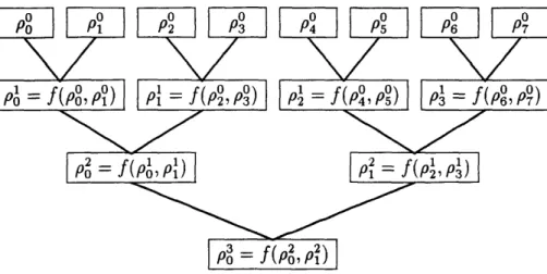
Function COMMIT(1K, r):

1. Append O's to the end of r until a string p whose length is c times a power of 2 is obtained. Say II = 23 r. Note that IPj < 21rl, and so a = O(log n).

2. Divide p into 2c segments of length K each, p = pao p o P2%-I (we callo...

the p°'s the segments of 7r, or of p).

3. Compress pairs of adjacent po's together, meaning: compute pl = f(po, po),

P

=

f(P, P), .. P2a-

1

=

f(P2-2,P2-)-4. Compress pairs of adjacent pl's together as above to compute p2 = f(p l, pl),

i

P1-

= f(p2, P3), .

.P2o-2_,

= f(Pa-l-2, P -1.

5. Continue in this vein until an complete 2a-leaf binary tree has been created, with R = p at the root (see figure 4-1).

6. Output the value 7R E {0, 1}' as a committal to the probabilistically check-able proof 7r.

P0 PP P2 P3 P4 P5 Pg P7

1 0 1 10 F

Pa = f(Po, P) 1Pi = f (PP) P2 4 , P P3 = 6, P

Pi

p

o

=

f(

=

Po3

1

PO fJ l iPi= P p

Figure 4-1: The tree computed to commit to Ir, if a = 3

Suppose the Prover sends the Verifier a K-bit string as a committal. Later on, the Prover sends the Verifier a string r, claiming, "My value was a committal to 7r." For COMMIT(-, ) to be worth anything as a committal scheme, we would like it to be impossible for the Prover to decommit any string other than a string 7r which the Prover was actually thinking of, and on which it ran COMMIT(-, ) to obtain its committal. This is not quite the case; however, it is infeasible for the Prover to pull off a crooked decommittal. Essentially, if the Prover can decommit to two distinct values relative to the committal 1Z, then it must have found a collision of f(.); to have probability 2-°(k) of finding such a collision, the Prover must evaluate 2n(k)

different values of f(.).

The type of commitment scheme we use here was first used in Merkle [21], for constructing a digital signature scheme. It was later used by Kilian in [19] for zero-knowledge proof protocols very similar to the "3-round pseudo-CS proofs" we present in section 4.2. Benaloh and de Mare [8] present an alternative method of committing to long strings which can be used in situations similar to ours.

security parameters also require more resources (computation, storage, communication, etc.) from the participants.

4.1.3 Decommitting part of a committed proof

It's not enough for us that COMMIT(., ) is a good way to produce a short committal to a string ir. We need something more- a way to decommit a single bit of ir without having to perform much communication. Let 0 < p < ITrl be the index of a bit of r,

and consider the function DECOMMIT(.,-, ) and the predicate CHECK-DCM(., -.,.-,).

The bottom line here is that it's about as difficult for a crooked Prover to con-vincingly decommit a bit that it wasn't thinking of when it made the committal 1Z as it would be to decommit an entire string r that it wasn't thinking of. The basic reason for the difficulty is identical, too- the Prover would more or less have to find

Function DECOMMIT('1K, 7r, p):

1. Compute the values pb which were computed in evaluating COMMIT(l", r).

2. Set i = LJ.

3. Write the path (in the binary tree) from p to the root pO as pjO, Pl, pja, where jo = i and ju+l = [j./2J.

4. Set D = pj°O P0j P l P2 p o 2 ... °2 a

-5. Output D as a decommittal of the bit rp.

Predicate CHECK-DCM(1, D, p, PR):

1. Write D as D = A o Bo o Al o B1 o o A,-_ o B,_1, where each Au and

each Bu has length eK.

2. Check that for u = 0, 1, ... , a - 2,

Au+ f (A,, Bu) if bit #u of [P/'rJR is a 0

f(Bu, Au) if bit #u of [P/IKJR is a 1

3. Check that 7 = f(A,_ 1, B,_1) if bit #(a - 1) of [p/14JR is a 0 f(B,- ₁, A,_1) if bit #(a- 1) of

[P/CJR

is a 1

4. If all a of the f(.) values computed check out as above, output 1 (accept the decommittal as valid); otherwise, output 0 (reject the decommittal).

an f-collision. We won't go into more detail about this here, since chapter 5 will provide about all the detail one can handle.

We see that a single decommittal has length 2ac.

4.2 3-round pseudo-CS proofs

We can take all the things we've built so far, and put them together in a 3-round proof system which needs very little communication, the protocol 3-ROUND PROOF(.,, ),

which is just a natural "conversion" of MAILBOX-PCP-PROOF(., .).

Like PCP-PROOF(.), 3-ROUND-PROOF(-,.,.) can be repeated multiple times to obtain more security. For the sake of efficiency, the same committal T1 can be used for each repetition (i.e., only steps 3-6 need to be repeated). Furthermore, all the repetitions can be done in parallel, so that the entire protocol still takes only three rounds.

Protocol 3-ROUND-PROOF(1K, x, w):

1. The Prover computes r = 7r(x, w).

2. The Prover computes R = COMMIT(1S, r) and sends to the Verifier. 3. The Verifier flips R(n) coins, and uses the result to pick q bit positions

71, 72,..., rq, in the proof that it wishes to examine. It sends 7r, 2,..., 7rq

to the Prover.

4. The Prover computes the decommittals Di = DECOMMIT(1, r, pi) for i =

1, 2,..., q. It sends the Verifier D1 o D2 o ... o Dq.

5. The Verifier checks that CHECK-DCM(1', Di,p, 1) = 1 for i = 1,2,.. ., q. If any of these does not hold, the Verifier rejects the proof.

6. Otherwise, the Verifier decides whether to accept or reject based on the values of the bits decommitted, as in an ordinary probabilistically checkable proof.

4.3 CS proofs, at last

It's now just a short step to CS proofs. In effect, CS proofs are obtained by taking the 3-ROUND-PROOF(., , ) protocol (repeated , times), and replacing the Verifier's coin-flipping with a random oracle (to get rid of the interaction in 3-ROUND-PROOF(., , )). We elaborate on this. Producing a CS proof with security parameter en (a "-CS proof") that (3w: P(x. w) = 1) requires two random oracles. One of them we have already seen, the random oracle f: {0, 1}2 _{{0, 1}'. We now add in an additional}

random oracle, g: {0, l} X {0,1} l {0 , 1}R(n),, (recall that n = xi). Then the function CS-PROOF(,, ) can be used to create CS proofs.

Carefully going through the code for CS-PROOF(.,-, ) reveals one other difference from 3-ROUND-PROOF(-,., .). Namely, CS proofs explicitly contain the random chal-lenge bits, g(x o R). In view of the fact that the string 1R is also contained in the CS proof, this might seem wasteful; however, it will simplify matters somewhat in section 5.3.

With everything we've put together so far, it's not hard to come up with a predi-cate CHECK-CS-PROOF(., , ) for the Verifier to use to check if a CS proof is valid.

Function CS-PROOF(1, , w):

1. Compute 7r = r(x, w).

2. Compute R = COMMIT(1N, 7r).

3. Evaluate g(x o R) and divide it into K "challenges" of length R(n) each,

g(xo R) = r

r

1

r o

o r,.

4. For each s = 1,2,...,c,

(a) Compute p-, p,..., p', the positions of the bits in ir that T(.,.,) would wish to examine, given inputs x and rs.

(b) Compute D? = DECOMMIT(1,r, pf) for i = 1,2,...,q.

(c) Set hs = D o D o. o D-.

5. Output the string R o rl o hi o r2 o h2 o ... o r, o h, as a -CS proof that

Predicate CHECK-CS-PROOF(1 x, ):.,

If CHECK-CS-PROOF(x, M, ) = 1, we say that M is a valid x-CS proof that

(3w: P(x, w) = 1). Note that this can hold even if there actually is no such witness

(i.e., valid CS proofs are not necessarily correct).

A little bit of simple arithmetic reveals that the length of a Ic-CS proof that (3w: P(x, w) = 1) is precisely K[1 + R(n) + 2arqK] = O(rK2_{logn). For convenience}

later on, we define the "CS Proof length" function Ap,WL(n, K) = I[1 + R(n) + 2aqK].

1. Write M as a concatenation M = 7i o o h o 2 o h2 o ... , o h,.

2. Divide g(x o 7) into xc pieces of length R(n) each, g(x o 1) = r o r2 ..o o r,.

3. For each s = 1,2,...,K, (a) Check that r = rs.

(b) Write h, as a concatenation h = D o D o... o Dq.

(c) Compute p', p... .. ,pq, the positions of the bits in r that T(.,., ) would wish to examine, given inputs x and r.

(d) Check that CHECK-DCM(1K, D ,p, 71) = 1, for i = 1, 2,...,q.

(e) Check that the values decommitted for rprp2,... 7rps would cause T(.,., ) to accept the probabilistically checkable proof7r, given inputs x

and r,.

4. If M passes all the checks above, accept the CS proof M (output a 1). Otherwise, reject M by outputting a 0.

Chapter 5

CS proofs of knowledge

As with other proof systems, there are two distinct parts needed to demonstrate that CS proofs can actually serve as proofs:

1. Some kind of completeness property, which ensures that an honest prover can convince a Verifier of any particular true statement with very high probability.

2. Some kind of soundness property, which ensures that a dishonest prover can't convince a Verifier of any false statement with nontrivial probability.

As mentioned earlier, in [22], Micali is concerned with CS proofs as proofs of

membership, and he demonstrates versions of these properties which he calls "feasible completeness" and "computational soundness." Feasible completeness means that not only can an honest Prover possessing an NP witness that x E L always successfully convince a Verifier that x E L, but in addition, it can do so in time poly(lx[, ).

Computational soundness means that a dishonest Prover, trying to convince a Verifier

of some false statement E L, can only succeed with an exponentially small (in I)

probability, unless it has so much computational power that it can make exponentially many (in ra) oracle evaluations of the functions f(.) and g(.).

In this chapter, we shall present our results on how CS proofs can be used as proofs of knowledge. As always, this requires proving a completeness property and a

Feasible completeness is sufficient for use in CS proofs of knowledge. We here present Micali's definition in a way which we feel clarifies how it can be used for to CS proofs of knowledge.

Let WL(.) and P(., ) be as usual (we fix WL(.) and P(-, ) for the duration of this chapter). Then feasible completeness means that:

1. Vxz {O, 1}*, if w is an NP witness that (3w: P(x, w) = 1), then

Pr(CHEcK-CS-PROOF(1r , M) = 1: M = CS-PROOF(1,x, w)) = 1.

2. The algorithms CS-PROOF(.,.,.) and CHECK-CS-PROOF(.,-, ) both run in polynomial time.

5.1 What about soundness?

Micali's computational soundness is not strong enough to show that CS proofs can be used as proofs of knowledge. We shall therefore propose and prove a new notion of soundness for CS proofs. In addition to being useful for its applications to digital signature schemes, as will be demonstrated in chapter 7, the notion is interesting in its own right.

If we consult the literature on zero-knowledge proofs, we see that there is a non-trivial difference between zero-knowledge proofs of membership and zero-knowledge proofs of knowledge (see Tompa and Woll [30], Feige, Fiat, and Shamir [12], and De Santis and Persiano [9]) which is similar to the distinction we face with CS proofs. It is not immediately obvious what it means for a protocol to "prove" that one of the parties "knows" an NP witness of some fact.

The three papers above all define a soundness property for zero-knowledge proofs of knowledge by saying that there must exist a "knowledge extractor," which is es-sentially an efficient algorithm which, given some form of control over running the Prover, can produce an NP witness of the fact to be proved.

formalize in a natural way what it means for an algorithm to "know" something. Given this, we might be tempted to make a "knowledge extractor" definition for CS

proofs, as well. Since [9] is about noninteractive proofs of knowledge, and we find

ourselves in a similar situation, it might seem reasonable to adapt their definition to our needs.

De Santis and Persiano present two types of "knowledge extractor" definitions for noninteractive zero-knowledge proofs of knowledge. The weaker definition involves the Prover having some particular x E {0, 1}' in mind, and trying to convince the Verifier that (3w: P(x, w) = 1). The stronger definition allows the Prover to "shop around" and generate an x E {0, 1}* and a proof together, which could conceivably give the Prover more opportunity to falsely prove that it knows an NP witness of some fact. In analogy with their definitions, we shall make two similar definitions of soundness later in this chapter: "computational soundness of CS proofs of knowledge" and "strong computational soundness of CS proofs of knowledge."

However, the "knowledge extractor" approach is not precisely the best way to

define soundness for CS proofs of knowledge. This is because, for CS proofs, as we

shall see, performing committals via random oracle tree-hashing makes it possible to actually have some idea of what a Prover is "thinking." Given this, it is more intuitive to define soundness in terms of the Prover "having in mind" an actual NP witness. The resulting definitions of soundness, although slightly differently motivated, turn out to be essentially equivalent to the "knowledge extractor" definitions. In addition, Micali's original "computational soundness" property follows easily from either of our versions of soundness.

Most of the remainder of this chapter is devoted to formalizing and proving our new notion of soundness for CS proofs.

5.2 Setting the scene

Fix n, b > 0 and K > 1. Let C be a circuit with no input bits and (n + Ap,WL(n, ) + b)

random-oracle nodes for g: {O, }' x {O, i}X ~ {0, 1}R(n)', and any number of other special nodes of any types. Call C's g(.)-nodes G1, G2, ... , Gt. Writing the output of

C as x o M o E, where xl = n, MI = ApwL(n, K), and EJ = b, we think of C as a circuit which tries to output a triple consisting of a value x E {O, 1}1 (we call x'

an instance); a valid -CS proof that (3w : P(x,w) = 1); and some b-bit auxiliary

output, E.

DEFINITION: f-node. An f-node is an f(.)-node which is a predecessor of Gi. Let Ci be the subcircuit of C induced by Gi. Since Gi has (n + K) inputs, Ci is a circuit with no inputs and exactly (n + e) output nodes. We observe that two such subcircuits Ci and Cj need not be disjoint.

5.2.1 f-parents and implicit proofs

For the following definitions, let Z < C, and let 77 be a K-component Lz-random variable (i.e., any function mapping 'Lz to Es).

DEFINITION: f-left parent in Z and f-right parent in Z. The f-left parent

and the f-right parent of in Z are defined as follows:

* If 7 is the output of at least one f(.)-node in Z, and if any two f(.)-nodes in Z which output q both have the same input, then the f-left parent and the f-right parent of 77 in Z are the first and last Ke bits of that common input, respectively. * If 77 is the output of at least two f(.)-nodes in Z with at least two distinct inputs, then the f-left parent and the f-right parent of 77 in Z are both equal to * (i.e., a sequence of *'s).

* If 77 is not the output of any f( )-node in Z, then the f-left parent and the f-right parent of in Z are both equal to *.

The f-left parent of 7 and the f-right parent of 7 in Z are K-component z-random variables. For any e e iz, if ?r(e) = *, then the f-left parent and the f-right parent

of 1 in Z also equal *,.

1. Set i70 = .

2. Define ro and - 1 to be the f-left and f-right parents of /0' in Z, respectively. 3. Define T7-_{0 and r/}- 2 _{to be the f-left and f-right parents of r} -_{l in Z, and}

define /`- 2 <sub>and 3`</sub>- 2 _{to be the f-left and f-right parents of rq}-_{' in Z.}

4. Continue in this fashion, defining and to be the f-left and f-right parents of qr in Z, until a tree similar to the one pictured in figure 4-1 is

obtained, with 7 's instead of p 's.

We say that the string

4

o ° ... o 71a is the implicit proof Z committed to

with a/.

4

is a z-random variable of the same length that a probabilistically checkable proof that (3w: P(x, w) = 1) should be (assuming that

lxJ

= n), once that

proba-bilistically checkable proof is padded to have length equal to xC times some power of 2. Indeed, as suggested by our terminology, the random variable is an attempt to reconstruct the probabilistically checkable proof that Z committed to via the short string r/. Of course, for a particular random variable 7, in a given execution e E Tz, it is quite possible that there is no such committed proof (i.e., that l/(e) was not

computed by tree-hashing any kind of string), in which case 1(e) is likely to be just a string of *'s; more generally, there can be gaps in the committed proof, which are filled in with *'s in (e).

Note that a string of *'s in an implicit proof can mean either of two very different things:

1. It was impossible to "trace back" the committal string 7(e) to a consistent

value for that part of the implicit proof, using only values of f(.) which Z had

evaluated.

2. At some point in the process of trying to "trace back" from nr(e) to the implicit proof, there were at least two distinct possibilities of how to trace back.

The former event means that Z does not "know" some probabilistically checkable proof which tree-hashes to the committal 77(e). The latter event means that, later

on, if r7(e) is used as a committal, then it might be feasible to decommit more than one value for a given proof bit. Because the latter event implies that Z has found an f-collision, it occurs very infrequently.

At long last, we define some particular random variables on c and fc,:

* Write the output of C as x or o r o ha o r2o h2 o or oh, o E, where

lxl

= n,

Ir[

= ,

El

= b, and for each s = 1,2,...,K, r,j = R(n) and h,j = 2acqK (this breaks up C's output into an n-bit x; the pieces that a valid -CS proof that

(3w: P(x,w) = 1 should contain; and an extra b-bit output). Recall that we

already defined M = o r o hi o r2 o h2 o ... o r, o h to be the CS proof output

by C.

* For

i =

1,2,...,K:

- Write the output of Ci (the input to Gi) as xi o yi, where 1xil = n and

lYI = K.

- Let i be the implicit proof Ci committed to with 'y.

Intuitively, we think of Ci as somehow computing an (instance, K - CS proof) pair (i.e., Ci's output), which will be used as input to the node Gi. Of course, the candidate K-CS proof may not be a valid CS proof for the candidate instance. Nonetheless, each g(.)-node does a priori give C a chance to output an instance and a valid K-CS proof of knowledge for that instance.

x, M, E, r, the r's, and the hs's are *c-random variables; and the yji's and the ~i's are 'tc-random variables.

5.2.2 Anthropomorphization of circuits

For the duration of section 5.2.2, fix Z < C.

Let f3, 3', 3o, and ]31 be K-component Tz-random variables. Let the Fz-event "Z

knows f(/o o /l) = /)" be