HAL Id: hal-02943086
https://hal.archives-ouvertes.fr/hal-02943086
Submitted on 18 Sep 2020
HAL is a multi-disciplinary open access
archive for the deposit and dissemination of
sci-entific research documents, whether they are
pub-lished or not. The documents may come from
teaching and research institutions in France or
abroad, or from public or private research centers.
L’archive ouverte pluridisciplinaire HAL, est
destinée au dépôt et à la diffusion de documents
scientifiques de niveau recherche, publiés ou non,
émanant des établissements d’enseignement et de
recherche français ou étrangers, des laboratoires
publics ou privés.
Fast maximum coverage of system behavior from a
performance and power point of view
Georges da Costa, Jean-Marc Pierson, Leandro Fontoura Cupertino
To cite this version:
Georges da Costa, Jean-Marc Pierson, Leandro Fontoura Cupertino. Fast maximum coverage of
system behavior from a performance and power point of view. Concurrency and Computation:Practice
and Experience, 2020, 32 (14), pp.0. �10.1002/cpe.5673�. �hal-02943086�
OATAO is an open access repository that collects the work of Toulouse
researchers and makes it freely available over the web where possible
Any correspondence concerning this service should be sent
to the repository administrator:
[email protected]
This is an author’s version published in:
https://oatao.univ-toulouse.fr/26363
To cite this version:
Da Costa, Georges and Pierson, Jean-Marc and Fontoura Cupertino,
Leandro Fast maximum coverage of system behavior from a
performance and power point of view. (2020) Concurrency and
Computation:Practice and Experience, 32 (14). ISSN 1532-0634
Open Archive Toulouse Archive Ouverte
Official URL :
https://doi.org/10.1002/cpe.5673
Fast maximum coverage of system behavior from a
performance and power point of view
Georges Da Costa
Jean-Marc Pierson
Leandro Fontoura-Cupertino
IRIT Laboratory, University of Toulouse, CNRS, Toulouse, France
Correspondence
Georges Da Costa, IRIT Laboratory, University of Toulouse, CNRS, Toulouse, France. Email: [email protected]
Funding information
FP7 Information and Communication Technologies, Grant/Award Number: CoolEmAll / 288701
Summary
This article proposes a methodology for constructing and assessing the quality of benchmark-suites dedicated to understand server behavior. Applications are multiple: behavioral models creation, power capping, abnormal behavior detection, model val-idation. To reach all the operating points of one server, an automatic operating range detection is necessary. To get the knowledge of the operating range, an exhaustive search of possible reachable states must be conducted. While many works use for this purpose only simplistic benchmark-suites in their research, we show in this article that using simple assumptions (leading to simple models such as linear ones) introduces large bias. We identify the bias due to individual hardware components. The key for understanding and modeling of the system behavior (from performance and power consumption points of view) is to stress the system and its subsystems on a large set of configurations, and to collect values spanning over a large spectrum. We define a cover-age metric for evaluating the covercover-age of measured performance indicators and power values. We evaluate different benchmarks using that metric, and thoroughly analyze their impact on the collected values. Finally, we propose a benchmark-suite providing a large coverage, adapted to general cases.
K E Y W O R D S
benchmarking, performance counters, power, system coverage
1
INTRODUCTION
Having a precise understanding of the behavior of servers is of utmost importance from many points of view, in particular with the emer-gence of very large-scale datacenters supporting the ever growing demand in services and applications. The complexity of such behavior comes from the large number of dimensions. Behavior encompasses not only system values like processor or memory load but also power consumption. The knowledge of power consumption of infrastructures is important for operators to compute their overall power demand or to bill customers based on the amount of electricity actually used. It can also serve operators to raise awareness on energy consumption to their users.
Deriving a model from system observation is a commonly used technique for constructing models. Machine learning methods learn the behav-ior of a system from a set of measured observations such as power consumption, key performance indicators coming from the server (performance counters) or from the operating system. Then these techniques build a model fitting the observations, for example, correlating the power consump-tion to the values of the key performance indicators. The need for having a large span of observaconsump-tions is therefore key for having good models. Machine learning is a data-driven approach, so the data used to create the models need to be representative, that is, they must cover the highest amount of system's configurations and devices' usage, ideally independently.
The span of usage of the server equipment is a knowledge useful also for the system operator. In particular, when Having a deep understanding of a server is also of use for operators of datacenters. When dealing with power, it is important to know the extent of power consumption range. Power capping enforced by an operator relying on partial information can lead to reduce the productivity of a datacenter since a conservative policy might be applied too often to prevent from exceeding the maximum allowed power drained from the electrical provider. Besides, knowing the normal behavior is helping the detection of abnormal behaviors leading to failures.
Benchmarks are used for stressing the components of a system, sometimes one at a time, sometimes more or less all together. Benchmark-suites from literature are proposed for specific use cases, not generic ones. They do not manage to cover all the performance indicators and power con-sumption span at once. They reflect the actual usage of resources in their target cases, but fail to reflect usages outside of their scope. Using these benchmark-suites for constructing generic models is not a wise option, since the derived models cannot fit observations outside the learning span. In addition, last but not least, researchers are in need of good coverage benchmark-suites in order to test their researches in the most complete way.
The main contributions of this work are the following:
•
after showing that a simple benchmark focusing on only one subsystem is insufficient to explore all possible power consumption, we identify the characteristics a generic benchmark-suite must integrate to effectively reach all possible resource consumption values;•
we show that the collected performance indicators and power measures have very different ranges of values depending on the benchmarks;•
we propose a generic benchmark-suite able to span over these ranges: This suite can generate inputs for assessing and modeling resource consumption of a machine;•
finally, we exhibit a methodology and we define a coverage metric in order to build a generic benchmark-suite able to span over large resource usage ranges.The rest of this article is organized as follows: In Section 2 we analyze the state-of-the-art in benchmark-suites used in the literature related to power consumption. In Section 3, we inspect the power consumption of subsystems, and we show that simple models do not work. We also show that each particular type of resource (such as memory, processor, network,…) has a particular and often independent impact on power consumption and on heat production and thus need to be taken into account to evaluate the quality of a benchmark-suite. We analyze benchmark-suite scrutiny using the proposed coverage metric and we construct a generic benchmark-suite for modeling power consumption in Section 4. We conclude and give perspectives to this work in Section 5.
2
STATE-OF-THE-ART
In many research works the benchmark-suites are dedicated and serve as particular use cases (web servers, HPC, and so on) and are pertinent for comparing system in that particular case. Poess et al.1give a good overview of energy related benchmark-suites. Industry-led benchmark-suites
such as TPC-Energy* and SPECPower and its successor server efficiency rating tool (SERT)†are such tools. TPC is dedicated to online transaction
processing (OLTP) and TPC-Energy naturally allows for ranking servers based on the number of processed transactions against the energy used for achieving these. Interestingly, this benchmark-suite is constructed by aggregating the results from different benchmarks (all related to OLTP) in one, advocating the fact that one benchmark does not cover all use cases, each stressing differently the overall system. SPECPower is a benchmark-suite for server side Java business applications. Its feature is to stress a system between 10% and 100% processor load (with 10% increments) and to cal-culate (for each load) the performance to power ratio. This allows comparing different servers to that metric. The SERT tool uses a set of synthetic workloads to test individual system components and provides power consumption data at different load levels: it follows the specification of the EPA energy star for server (initialized in 20092) addressing less specific use cases toward more generic workloads. In the context of high-performance
computing (HPC), the Green 500 list3is ranking machines using the LINPACK benchmark: The list is constructed from the number of Flops
(float-ing point operations per second) achieved per s(float-ingle Watt, while the LINPACK benchmark is supposed to represent a generic HPC application. This statement has been challenged, in particular with the appearance of new architectures, leading to new HPC benchmarks (for instance, the high-performance conjugate gradient4). Another point making the benchmarking difficult is that it has been observed that the same system can
con-sume different power (depending on its manufacturer): As an example,5Pentium processors can consume up to 10% difference while being identical
(on data-sheets).
While recognizing the importance of each of these for comparing infrastructures, they do not provide enough coverage to solve the use cases described in the introduction. In fact, it would be necessary to use at least all these benchmark-suites to stress the different components of a system, from hardware components to operating systems, in different conditions. Few works have been done to produce a scientific generic approach. The
*http://www.tpc.org/tpc_energy/ †https://www.spec.org/power/
TA B L E 1 Summary of synthetic benchmarks used for hardware
profiling Name Description
C0 Set processor's active mode (C0-state) CU Stress CPU's Control Unit
ALU Stress CPU's Arithmetic Logic Unit FPU Stress CPU's Floating-Point Unit
Rand Stress CPU's FPU using random number generation L1 L1 data cache access (read/write)
L2 L2 cache access (read/write) L3 L3 cache access (read/write) RAM RAM memory access (read/write) iperf3 Stress IP Network (upload/download)
importance of coverage is well known in other fields where this metrics is used as an indicator6for reliability, but is not to our knowledge yet used
for the span of impacts of benchmarks and benchmarks-suites on servers.
3
IMPACT OF DEVICES ON ENERGY
The first step in defining a benchmark-suite is to perceive how energy is consumed by the target system's devices. It requires the development of synthetic benchmarks to measure the impact of each system's device on the total power. The complete list of benchmarks used for device profiling is found in Table 1, more in depth description will be given later in this section.
The platform used to perform our experiments is the Resource Efficient Computing System 2.0 manufactured by Christmann GmbH, allowing for high precision power accuracy on an 18 nodes machine.7The profiling presented in this section executed the synthetic
bench-marks during 50 to 100 seconds with a power sampling rate of 1 Hz and milliwatt precision. This large amount of samples enabled us to estimate the confidence interval of the measurements, based on the central limit theorem, to ensure that our results are statistically acceptable.8
3.1
Base system
Server infrastructures consume a substantial amount of power even when they are idle.9Base system's power refers to the power dissipated when
nodes are idle, that is, no tasks are being executed besides the operating system. The base system power consumption is useful to create power models at system- and process-level.
In the following experiments, we used a motherboard using the Intel Ivy-Bridge i7-3615QE (4 cores, 16 GB mem, 1.2-2.3 GHz, boost enabled) processor which is a high-performance processor used in a high density context (9 motherboards in a 1U rack). It is on a dedicated PCI-Express moth-erboard node without storage. All power consumption values in the following are measured before power supply unit (PSU) but are corrected10
in order to take into account PSU efficiency impact and thus measurements can be considered to be at the motherboard level. PSU impact has been removed in order to evaluate the impact of benchmarks on the hardware without the bias of nonconstant efficiency of PSU which depends on the particular nodes used. Temperature readings are obtained though the CPU advanced configuration and power interface (ACPI) interface and only account for processor temperature. The static power at idle dissipated by the i7 motherboard is 32.8 W. Fans on this moth-erboard are constantly on, and we removed their constant power consumption. They are not in a control loop linked to the processor or board temperature.
As most datacenters separate storage and computing infrastructure, most servers in datacenters do not have attached hard drives or solid storage drives. Thus, in the following, local I/O will not be investigated.
Measuring power consumption is done using external hardware and must be precisely correlated with system monitoring and must take into account several bias (such as time jitter, imprecision of hardware measurement, and so on). We followed a measurement methodology11to cope
with this bias. The frequency of measurement is 1 second, sufficient for linking power consumption to behavior of HPC applications usually run-ning from several minutes to several hours. This frequency prevents from investigating very fast phenomenon such as the physical latency between temperature and power leakage.
0 25 50 75 100 35 40 45 50 55 60 65
Core 1 Core 2 Core 3 Core 4
Processor usage (%) Average Po wer
(
W)
,σ< 1.35 ALU FPU CU RandF I G U R E 1 Workload power profile for i7 motherboard. For the same measured load, power consumption depends on the exact application
3.2
Processor
The processor is claimed to be the most power consuming device in a computing system.12-16Recent processors have different features to
facili-tate operating system's ability to manage processor power consumption. The ACPI17defines power (C-states) and performance states (P-states)
that control the operating mode of a processor, turning some components off when they are idle and changing the cores' frequency dynamically, respectively. This section explores some processor's features, while profiling its power consumption.
First we analyze processor's workloads' impact on power dissipation. In order to decouple processor from system power, a set of four syn-thetic benchmarks were implemented avoiding the use of other components. These benchmarks stress each processor's main components:18
control unity (CU), arithmetic logic unit (ALU) and floating-point unit (FPU). Given the impact of the random number generation, a fourth bench-mark was developed to exploit it (Rand). CU continuously executes a NOP operations (while(true);); ALU and FPU execute integer and floating-point operations, respectively; and Rand executes floating-point operations using a random number as an input variable. All bench-marks were compiled using GCC version 4.4.7 without optimization (-O0) and verified using objdump -d to guarantee that the final executable binaries fit the expected assembly code. This low level of optimization prevents the compiler from simplifying the benchmarks to a simple NOP code.
Each synthetic benchmark was executed increasing the number of active cores and their usage in 10% steps during 50 seconds. For the i7, one core was used up to 25% load, then two cores from 25% load to 50% load, then three cores between 50% and 75% load and finally four cores when the load was higher than 75%. The cores frequencies were kept in their best performing values, that is, Boost. Figure 1 summarizes the results of this experiment.
One can observe from Figure 1 that all workloads share the same trend, that is, the power increases according to the processor's usage for all cases.
The i7 nodes present a power variation of up to 34.2 W, according to their usage. This means that the maximum power consumption of a system doubles from idle (≈33.1 W) to a fully stressed state. The most complex the architectures, the more power savings are available, but also incurring a higher variability of their power consumption.
Another interesting aspect of this experiment is the nonlinearity between power and CPU load, shown in Figure 1. The first stressed core (pro-cessor usage less than 25%) increases at a higher rate than the following ones. This goes against several model proposals that consider the power as being linear to the CPU load,19-22also called CPU-proportional models. These models are usually accurate when a processor has a single core. When
several cores are present, the exact available computing power depends not only on the maximal computing throughput of each core, but also on the thermal budget. This phenomena has already been described23in the context of many-core architectures.
Moreover, the power profiles differ for each workload. Rand presents the higher power consumption for the same processor usage, while the power of ALU and FPU are quite close for all stressed levels. Depending on the workload, the power of an i7 can reach up to 14.2 W difference at maximal load, which represents 20% of system's power consumption or even 40% of the dynamic power, that is, while removing the idle power. Once again, CPU-proportional models do not take this into account.
Thermal dissipation and power consumption are intrinsically related24,25thus, the next investigated aspect was the processor's temperature.
Processor's core temperature was evaluated by executing the Rand benchmark concurrently in all cores during 350 seconds and then letting them idle for the same time. As the time variable on this experiment is important, the experiment was repeated 10 times and the SD and median of each data point was calculated. The results presented in Figure 2 show a high correlation between power and processor's temperature variation, reach-ing a correlation coefficient of 0.97. However, the impact on power is not very large. After 350 seconds of the stress phase execution, the power
Time (s) Median Pow er ( W ) ,σ< 14.23 0 70 140 210 280 350 420 490 560 630 700 35 45 55 65 30 40 50 60 70 Median A ver age Core T emper ature (°C)
Stressed Cores Idle
Power Temperature CPU usage
F I G U R E 2 The impact of temperature over the dissipated power on a i7 motherboard
F I G U R E 3 Power profile of data access in several memory levels
increased≈1.5 W, while when put in idle mode, it decreased only≈0.5 W. This experiment shows that temperature actually influences the power, but may not be a crucial key variable.
Distinct memory level accesses were also evaluated by running the same code while accessing different memory positions to force specific memory accesses. The execution of the same code allows the comparison of memory accesses while the processor behaves similarly. Synthetic benchmarks L1, L2, L3, and RAM were developed to guarantee memory read/write accesses exclusively to their respective memory level, that is, L1 only uses L1-data cache accesses, L2 only L2 cache accesses and so on. More generally, using library like hwloc26these microbenchmarks can detect easily cache sizes. All benchmarks have the same processor usage which corresponds to a single core fully stressed. Once again, processor's frequency was set to operate at its highest frequency. i7 processors have three layers, where L1 and L2 are core specific and L3 is shared among all cores. If memory intensive applications are run on all cores, the contention on the memory bus can lead to an increase in execution time. The results presented in Figure 3 show that the memory access pattern has also a large impact on power consumption. Increasing time and power leads to have a substantial influence on the overall energy consumed. One can observe that, for all memory levels, writing accesses are more expensive than reading ones. In the i7 motherboards, the average power difference between the L1 and RAM memory is 1.84 W for read access and 4.4 W for write access. Power saving techniques are important features available in recent hardware. These techniques require more complex architectures and their implementation varies across vendors and target consumers. The most famous techniques are processor's idle (C-states) and performance (P-states) power states, both are evaluated as follows.
Idle power states impact on power is measured by comparing the idle system in active state (C0) and on its deepest idle state (CX). The level of the deepest idle state depends on the processor's architecture, for i7 motherboards it is C7. The highest the C-state, the more components are inactive. For instance, C4 state reduces processor's internal voltage, while C7 also flushes the entire L3 cache. In this experiment, the system is set to operate at its highest frequency. In order to force the processor to be always active, processor's latency was set to zero by writing on the /dev/cpu_dma_latency setup file. The results in Figure 4 show the power and processor usage for C0 and CX of i7 motherboards. One can see
F I G U R E 4 Power consumption (left) and processor usage (right) for an idle system when it is in active (C0) and in its deepest (CX) idle state
F I G U R E 5 Frequency scaling impact on power during the execution of Rand benchmark in all cores and while idle in C0 and CX
that processors' usage are kept low (near zero), evidencing that in both cases the system is idle. However, large power savings can be noticed. For the i7 motherboard the savings reach 23.54 W between C0 and CX state, putting the light on the importance of taking into account the time spent in idle states as a variable when observing recent hardware.
The second power saving technique to be evaluated was the P-states, also referred to as dynamic voltage and frequency scaling (DVFS). DVFS was evaluated by running the Rand benchmark in all cores and modifying the operating frequency to all available frequencies. For the i7 nodes, Intel Boost Technology may operate at up to 3.3 or 3.1 GHz when stressing one and four cores, respectively.27Figure 5 shows the average power when
running Rand benchmarks and leaving the system idle in C0 and CX for each frequency. The results show that the power dissipated in the deepest idle state (CX) is barely the same for all frequencies in all motherboards (32.92 and 32.84 W). In addition, by comparing the idle power dissipated in C0 and CX, one can see that power savings due to the idle states can reach from 8.42 to 23.53 W depending on its frequency in the i7 motherboard. The impact of using the Boost technology is very important and represents for the Rand benchmark a difference of 22.65 W when compared with the minimum allowed frequency (1.2 GHz) and 13.58 W to the maximal clock rate (2.3 GHz).
3.3
Random access memory
The profile of memory accesses described earlier showed that accessing the RAM highly increases the power cost of an application, when com-pared with any cache-level. In the current experiment, we profile RAM accesses to analyze the impact of its allocation size. This procedure gradually increases the size of the total allocated resident memory from 10 times the size of the last level cache memory to the maximum allowed memory
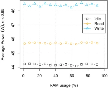
F I G U R E 6 Random access memory allocation impact on system's power
allocation. The minimum and the step size of memory allocation are 60 Mb to 14 Gb with 1 GB step. The memory allocation was tested with three cases: read, write and idle (no access to the RAM). All these cases kept one core of the system busy, that is, 25 % of processor usage for i7 while being at maximum frequency.
Figure 6 presents the average power consumption in function of the total RAM allocated. The SD of the power samples is low, that is, less than 0.65. The results of Figure 6 show that the average power is completely in line with the results of cache profile (Figure 3) for all memory accesses and resident memory size. As one can see, the most important is not the amount of allocated memory, but the type of access that is realized by the application. The power consumption varies up to 4.47 W. However, as some technologies intend to switch memory ranks on and off,28this may
change the impact of allocation size.
3.4
Network interface card
Networking is said to be crucial for wireless devices, but is often neglected in wired systems for most power modeling approaches. Network inter-face card (NIC) impact on power consumption was evaluated by controlling the download and upload throughput. Since network performance depends on the available processor and memory, during the networking transactions the usage of these resources was monitored along with sys-tem's power consumption. The monitoring of additional resources will allow us to identify if the variations on the consumed power comes from the NIC itself or from the related devices. This experiment explored the iperf3 tool‡to stress the IP network under several bandwidths in both upload
and download directions. To allow the power measurement of a single node, a server was instantiated on a separate node to communicate with clients instantiated on the evaluated motherboard. The network was then stressed in a 10% increasing steps scenario and limited by NIC's physical limitations, that is, 1000 Mbits/s on the gigabit Ethernet card as the increasing step.
Figure 7 presents the average power and the processor's and memory's usage. The i7 motherboard reaches up to 895 and 884 Mbits/s for upload and download, respectively. It is important to notice that an evaluation of NIC's power from an outlet meter, will measure not only the NIC but also processor and memory consumption. When running these setups, we observed that the CPU usage was always below 2.5%. Results from Figure 1 show that the most power expensive benchmark (Rand) consumes in average 34.2 W at 2.5% load. As the processor usage does not exceed this amount, the results of Figure 7 show that the impact of network usage can surpass 3 W. The low processor and constant memory usage during these experiments showed that actually the network does not have a constant power usage as proposed in some of our previous experiments.29
3.5
Summary
The power profile of a server cannot be understood using only the load of its processor. Even if this load is the largest contributor of the dynamic power consumed by the whole system, Table 2 shows that memory and network usage have a large impact. In addition, even for the processor, depending on the exact workload, a fully loaded system can have different power consumption levels.
F I G U R E 7 Network usage impact on the overall power consumption for Gigabit Ethernet cards. On left, reference of maximum power consumption on cpu-related benchmark at 2.5% load is shown. On right allocated memory is shown as being constant and processor is shown to stay under 2% during the whole experiment
TA B L E 2 Maximal impact (in Watts) of each device on motherboard's power consumption
Base Processor RAM NIC
Motherboard Power Load Temp Cache Cstate Pstate Access Alloc. Down Up
i7 10.9 34.0 1.5 3.0 24.0 22.0 4.5 0.0 3.0 2.8
Each of the presented microbenchmarks have a particular impact on power consumption with different timescale (leading to different temper-ature impact). In order to compare benchmark-suites, it is thus necessary to compare their usage of all type of resources from memory-busses to cpu usage.
4
WORKLOADS' SCRUTINY
Data-driven approaches for power modeling require the execution and monitoring of workloads to create and validate the models. Selecting a generic dataset to be learned is often a nontrivial task since it must ensure that it encloses enough samples from various operating points. This section describes the methodology to create and evaluate such workloads, dividing them into a generic workload proposal and some real world use-cases. The workloads were selected to provide a good coverage of the software usage of computing systems, representing standalone and dis-tributed applications. The generic workload covers several low power cases, representing use cases such as cloud providers (data base and web servers), while HPC applications provide high power dissipation characteristics exploring data locality and communication aspects.
4.1
Description of workloads
4.1.1
Generic workload
Based on the expertise acquired when developing the experiments presented in Section 3, we designed a synthetic workload. This synthetic work-load was generated by combining the synthetic benchmarks proposed in Table 1 according to their impact on the power consumed by the compute box. This workload is divided into several basic workloads according to their target component: processor, memory, network or whole system. Each of these basic workloads are executed varying the system's configuration to force the processor to operate in three different frequencies: minimal (1.2 GHz), medium (2.0 GHz), and maximal (Boost, up to 3.3 GHz).
The processor workload stresses the subdevices of each processor's core at several loads. First the system is kept idle in both active (C0) and deepest (C7) idle power states. The C0 state is achieved by running the C0 benchmark. Then, the processor workload run the CU, ALU, and Rand benchmarks consecutively, varying their processor load in 10% steps for each core.
The memory workload tackles L2, L3 caches, and RAM memory accesses for reading and writing. The L1 data cache is neglected since previous experiments showed that its impact on the power is almost null, consuming the same power as other CPU-intensive workloads. Thus, this workload runs the L2, L3, and RAM synthetic benchmarks.
F I G U R E 8 Generic workload proposal based on synthetic benchmarks to stress the processor, memory and network, along with a mixed setup to stress all devices concurrently
TA B L E 3 Execution time for each benchmark
Benchmark Generic Pybech OpenSSL C-Ray Gmx-Vilin Gmx-PolyCH2 Gmx-Lzm Gmx-DPPC
Time (min) 70 0.6 3.5 2 0.3 0.5 1.6 8 Benchmark HPPC_5k HPCC_5k_dist HPCC_10k HPCC_10k_dist HPCC_20k HPCC_20k_dist
Time (min) 0.3 2 1.9 6 12 19 Benchmark NPB_A NPB_A_dist NPB_B NPB_B_dist NPB_C NPB_C_dist Time (min) 1.9 2.4 9.8 12 44 43
The network interface is stressed through uploading and downloading data at different bandwidths. Although the power dissipation during the upload and download are equivalent (Figure 7), we included both transactions in this workload due to their difference on processor's load. This workload executed the iperf tool to download and upload data at a maximum speed of 200, 400, and 1000 Mbits/s.
Finally, a combined workload intends to stress the system at its maximum power consumption. The system workload is composed by Rand running on all cores; C0, L3, and RAM in single threads; and iperf to download data from another server with no bandwidth limit.
The power profile of the generic workload is shown in Figure 8. One can see that the power may significantly vary according to system's setup and workload. While most authors only evaluate their models under well-known behavior workloads/setups, we propose a workload which highly varies the power to achieve a broader behavioral span. Ideally, the results of the generic workload should be uniformly distributed, but, as the variables are not independent, this cannot be achieved. It has to be noted that the thermal effect shown in Figure 2 is not visible due to the timescale.
4.1.2
Other benchmarks
Several other benchmarks are evaluated in the following experiments. Cloud applications are represented with pybench,30stress (classical Linux
benchmark), and OpenSSL31benchmarks. HPC applications are represented by C-Ray (raytracing benchmark), Gromacs32(GROningen MAchine for
Chemical Simulation), HPC Challenge suite (HPCC)33(featuring the HPL, DGEMM, STREAM, PTRANS, RandomAccess, FFT, b_eff benchmarks), and
NAS Parallel benchmarks34(NPB). HPCC and NPB are distributed and are used in two different configurations, one in multithread on a single node,
one in a distributed configuration using the Gigabit Ethernet network. Depending on the particular benchmark, the running time varies from a few seconds to several minutes. Table 3 shows the running time for each benchmark. One can note that the execution time of the generic workload lasts 70 minutes, which must be compared with the duration a cocktail of the other benchmarks would have taken (the whole set of other benchmarks lasts 170 minutes).
4.2
Power, processor, and network profile
The power profile of a same application may vary according to its setup configuration. During the execution of each workload, the power consump-tion, processor's and NIC's usage were profiled. These performance indicators were chosen since many researchers consider the power as a linear function of the processor usage, neglecting the network impact.
02 5 5 0 7 5 1 0 0 Usage (%) Execution time (m) P o w er (W) 0.0 0.5 1.0 1.5 35 45 55 65 75
Power CPU Usage NIC Usage
(A) C-Ray: size 2560x1600
02 5 5 0 7 5 1 0 0 Usage (%) Execution time (m) P o w er (W) 0.0 0.1 0.2 0.3 0.4 0.5 35 45 55 65 75
Power CPU Usage NIC Usage
(B) Gromacs: Polyethylene in water (Gmx-PolyCH2)
F I G U R E 9 Multithreaded (four cores) CPU intensive workloads' profiles
02 5 5 0 7 5 1 0 0 Usage (%) Execution time (m) P o w er (W) 0.0 0.5 1.0 1.5 35 45 55 65 75
Power CPU Usage NIC Usage
(A) N=10,000; standalone 02 5 5 0 7 5 1 0 0 Usage (%) Execution time (m) P o w er (W) 0 1 2 3 4 5 6 35 45 55 65 75
Power CPU Usage NIC Usage
(B) N=10,000; distributed
F I G U R E 10 HPCC benchmarks' profiles standalone (four processes) and distributed (six processes) modes
When dealing under a controlled environment, the processor's load can be used as a good predictor for the power dissipation for some work-loads. For instance, Pybench, OpenSSL, C-Ray, and Gromacs, which were executed as standalone applications, where the processor's cores operated under the same constant frequency present a high linear correlation between power and processor's usage, see Figure 9 as an example. For these limited CPU intensive standalone cases, a simple linear model such as P= 0.31 ∗CPUu+ 35.91, where P is the power and CPUuis the processor's
usage, provides a correlation of 0.99, representing an almost perfect fitting. This applies to most of the CPU intensive cases, nevertheless, for more complex cases, such as HPCC and NPB (Figures 10 and 11) a significant variation on the power consumption can be noticed even if the processor and network usage are constant.
The generic workload, presented in Figure 8, shows that processor usage alone is not enough to model the power consumption of a com-puter. The CPU intensive phase repeats the same processor usage profile 9 times, although the power consumption changes at each time. The memory phase keeps the same processor's usage, while the dissipated power changes once again; a similar behavior can be seen in the NIC and All phases.
Another important aspect to be considered when using these benchmarks to learn new models is their power range. Figure 12 presents a box-plot of each workloads' power consumption. From the box-plot we can see that the power profiled by the generic workload is quite far from the HPCC, NPC, and Gromacs workloads. In other words, the generic workload alone in not suitable to be used to learn a model that will be later used to estimate the power of such workloads because it does not cover their range of outputs.
The proposal of a generic workload enclosing a wide range of use cases is not trivial. The previously described workloads are heterogeneous, as can be seen through the diversity of their profiles. One can realize how tough is to generate a generic workload by analyzing the range of values that each variable reached during the execution of a workload and comparing it with another workload execution. The number of collected variables is 220 during the execution of the workloads. Multiple sources provide these data: power consumption using an external power-meter, system vari-ables using collected35tool (encompassing memory, processor, network usage, and operating system values such as number of context switches, I/O
0 2 55 07 5 1 0 0 Usage (%) Execution time (m) P o w er (W) 0 10 20 30 40 35 45 55 65 75
Power CPU Usage NIC Usage
(A) Problem size C; standalone (4 processes)
0 2 55 07 5 1 0 0 Usage (%) Execution time (m) P o w er (W) 0 10 20 30 40 35 45 55 65 75
Power CPU Usage NIC Usage
(B) Problem size C; distributed (8-9 processes)
F I G U R E 11 NPB benchmarks' profiles in standalone and distributed modes
F I G U R E 12 Mean and SD (box plot) of power consumed by each benchmark. Individual circles are outliers showing the total span of power consumption
state). The variables used in the following experiments encompass all the available one these tools are able to monitor, hence reducing the possible bias of an a priori selection.
Table 4 shows the frequency of variables of each earlier described workloads that are out of the range of values of a reference workload. Each column of the table corresponds to a given reference workload, so the table shows how many variables of the row (comparing) workload surpass the ranges of the column (reference) workload.
Definition 1. The relative coverage metric coveragerelative(benchmark,benchmarkreference)counts the number of variables for which benchmark is out
of the bounds of the reference workload (benchmarkreference). It is computed as follows§:
coveragerelative(bench, benchref) =
∑
variable∈V
1min(variable(bench))<min(variable(benchref)) ∨ max(variable(bench))>max(variable(benchref)) (1)
with V being the set of all the monitored values, and variable∈V the monitored data for a particular variable. As an example, if variable is
cache-misses and bench is generic, then variable(bench)will be cache-misses(generic), a vector of all the monitored cache-misses for the generic benchmark.
In this formula, a 1 is added each time either the minimum or the maximum of the comparing workload (bench) reaches values which are not reached by the reference workload (benchref). The lower this value, the better the coverage of the reference. Indeed, if the value is very low, it means
the reference benchmark behavior encompasses most of the behavior of the other benchmark, leading to a good coverage of the variables span.
§1
TA B L E 4 Number of variables of the comparison benchmarks which go out of the bounds of the reference benchmark Ref. Comp. N1 N2 N3 N4 N5 N6 N7 N8 N9 N10 N11 N12 N13 N14 N15 N16 N17 N18 N19 N20 N1-Generic 0 183 181 169 181 184 172 166 170 160 162 161 164 160 164 156 164 154 161 159 N2-Pybench 12 0 99 93 97 103 83 73 75 56 66 63 64 56 64 54 64 48 60 58 N3-OpenSSL 11 118 0 87 98 111 82 65 83 53 60 58 59 54 55 51 62 47 63 52 N4-C-Ray 24 136 131 0 141 149 119 107 99 85 86 89 88 83 96 79 92 74 87 90 N5-Gmx-Villin 15 124 111 87 0 96 58 33 53 18 19 19 16 17 18 20 21 12 18 17 N6-Gmx-PolyCH2 18 123 104 89 103 0 55 34 53 19 21 20 19 18 22 15 22 13 24 15 N7-Gmx-Lzm 35 134 126 103 147 145 0 37 59 17 22 23 17 13 29 13 28 14 23 19 N8-Gmx-DPPC 44 146 144 117 171 167 155 0 71 51 45 56 42 32 49 33 48 24 39 38 N9-HPCC_5k 27 141 140 113 153 152 148 137 0 113 113 111 84 88 109 45 96 27 95 87 N10-HPCC_5k_dist 48 153 152 130 172 176 174 155 92 0 95 110 75 78 107 43 97 33 93 90 N11-HPCC_10k 46 145 146 129 170 173 167 152 87 102 0 115 79 89 122 51 100 38 87 87 N12-HPCC_10k_dist 50 148 147 129 169 174 169 146 89 89 81 0 59 67 106 47 94 30 97 88 N13-HPCC_20k 46 146 144 129 171 174 171 154 115 117 118 125 0 102 140 73 123 49 119 122 N14-HPCC_20k_dist 51 152 151 134 174 176 175 162 115 117 107 128 83 0 140 75 123 51 125 114 N15-NPB_A 46 148 151 122 169 169 159 145 93 88 76 83 55 59 0 40 78 25 70 68 N16-NPB_A_dist 56 164 161 145 186 186 187 179 156 165 153 163 126 129 165 0 148 65 143 140 N17-NPB_B 51 149 154 132 178 180 170 156 118 112 98 108 77 78 123 60 0 28 91 91 N18-NPB_B_dist 57 160 158 143 178 178 179 173 166 165 162 170 150 153 173 134 174 0 163 154 N19-NPB_C 55 154 153 133 179 176 174 162 121 116 113 109 85 80 132 67 103 45 0 100 N20-NPB_C_dist 56 154 154 126 178 175 173 160 114 113 111 114 83 89 131 67 109 50 101 0 Average 39 146 142 122 159 160 146 126 102 92 90 96 75 76 102 59 92 44 87 84 SD 16 15 20 22 29 28 43 51 35 47 44 46 40 42 49 36 44 32 43 43
Note: The lower, the better the quality of the reference benchmark. Bold values indicate which reference workload has the best coverage for a comparing
workload.
The Table 4 shows the values of coveragerelativefor the benchmarks. For instance, pybench contains 12 variables greater or smaller than the range
of the generic (reference) workload meaning coveragerelative(generic,pybench) = 12. On the other side, the generic workload has 183 variables
out of the bounds of the pybench (reference) workload, that is, coveragerelative(pybench,generic) = 183.
Definition 2. The coverage metric (coverage(benchmark)) is the mean value of all relative coverage with a constant reference benchmark. The
cov-erage metric helps to understand the relative quality of one particular workload compared with all the others. It evaluates, for each observable variable, the exploration of the set of possible values. It is defined in the following equation:
coverage(benchmark) = 1
|B| ∑
b∈B
coveragerelative(b, benchmark)
where B is the set of all benchmarks.
In Table 4, the reference workload that provides the best coverage for a comparison one is shown in bold. From these results we can see that, even if the generic workload is out of the range of power for the other workloads (Figure 12), it has the best coverage at the variables' perspective, having an average of 39 over 220 variables out of its range with a small SD. The coupling of different workloads in order to propose a generic covering work-load set is therefore necessary and the proposed coverage metric can serve as an indicator to help decide on which workwork-loads have to be included in such a generic covering workload. Overall, the first column of this table is the evaluation of each benchmark compared with generic showing that
learn generic apache apache_perf c−ray openssl pybench stress gmx_polyCH2 gmx_villin gmx_dppc gmx_lzm MAE (W) 0246 8 10 14
Case 1 Case 2 Case 3
learn hpcc_A hpcc_A_dist hpcc_B hpcc_B_dist hpcc_C hpcc_C_dist npb_A4 npb_A8_dist npb_B4 npb_B8_dist npb_C4 npb_C8_dist
MAE (W)
0246
8
10
14
Case 1 Case 2 Case 3
F I G U R E 13 Residual's based reduced ANN power models' comparison for each learning case after workload reexecution. Case 1 has been obtained with a learning based only on the generic benchmark; Case 2 with a selection of benchmarks; Case 3 with all benchmarks
the coverage of generic is good for each of the benchmarks. The first line is the evaluation of generic compared with each benchmark showing that none of the other benchmarks are able to represent the same span of values as generic.
It is then possible to generalize the coverage metric to a benchmark-suite by merging the variables of each benchmark included in the suite when computing the coveragerelativeequation.
4.3
Using the coverage metric for assessing the impact of benchmark-suites on learning techniques
As the quality of models produced by machine learning is sensitive to the quality of the learning dataset, it is a good show-case for the coverage metric. To illustrate the impact of coverage on learning methods, we trained three artificial neural networks (ANN) using the data obtained from three benchmark-suites for the learning phase to produce three ANN-based power models. Figure 13 shows the quality of the resulting ANN-based power models using the different learning sets (called case 1-3). It exhibits the error of the resulting power models for new execution of all the benchmarks (ie, different from the data used for learning) compared with the actual measured power. A lower error means that the produced model is closer to the real power consumption.
The three benchmark-suites have different coverage metric values: The first benchmark-suite (case 1) is the generic one, the second benchmark-suite (case 2) is composed of the generic benchmark along with one benchmark of each category (pybench, openssl, c-ray, one of each type of HPCC, one of each type of NPB, one gmx), and the third benchmark-suite (case 3) is composed with all benchmarks together. From Table 3, we see that the time needed are 70 min for case 1, 136 min for case 2, and 240 min for case 3.
Figure 13 shows that increasing the coverage of data for learning improves the quality of the ANN at the price of the time needed to acquire the learning set. As the coverage of the generic workload is already large, adding more data to the learning set through either particular applications (case 2) or all applications (case 3) improves marginally the quality of the resulting artificial neural network. It has to be noted that particular observations can differ from the overall result, when sometimes case 1 obtains slightly better results than case 2 or case 3. To prevent such corner cases, we used numerous benchmarks to have a better quality of the overall result.
The coverage metric for case 1 is 39 as shown in previous section with a global MAE of 2.31 W (computed on the execution of all the available benchmarks). The coverage metric for case 3 is 0 by construction (as the reference benchmark-suite include all benchmarks in this case) with a global MAE of 1.36 W. The coverage for case 2 is 12 with a MAE of 1.73 W, showing that with a better (lower) coverage value, the machine learning will be better.
4.4
Summary
In this section, we proposed a methodology in order to build a suitable benchmark-suite that will stress a server system comprehensively. The methodology consists in (i) choosing the set of variables to observe during the execution of workloads (possibly representative of the applications that will be executed on that system). (ii) execute the set of workloads and collect values during the execution (iii) compute the coverage metric for each comparing and reference workload based on the collected values (iv) analyze the coverage metric in order to select the most promising set of
workload that will cover at most the span of values of the observed variables. This set constitutes the generic covering workload to execute in order to have the best coverage of the selected variables within the lowest duration.
5
CONCLUSION AND PERSPECTIVES
This work demonstrates the particular need of research in energy efficiency in datacenters concerning benchmark-suites. For classical studies, most of the time, simple benchmarks are sufficient. For taking into account power in experiments, a new generation of benchmark-suites are needed.
This research work proposes a benchmark-suite that encompasses a large variety of resource impact, spanning a large range of power consumption. It also proposes a methodology and the coverage metric necessary to build a better benchmark-suite.
Using the proposed benchmark-suite, it becomes possible to work on machine learning methods to propose new models of servers power con-sumption using simple system-level sensors. Datacenter operators can also know the full range of behavior of their infrastructure, leading to better management and easiest detection of anomalies.
The next steps will be threefold : First defining a self-coherent generic benchmark-suite with a maximum coverage using only simple synthetic benchmarks instead of using applications, associated with a fast execution and a time limit for benchmarking. Second will be to introduce another metric which is the density of coverage, helping to understand how the span of values of the observed variables are representative of the execution of a whole application. Most applications described in this article show a trend of having 100% load. From a machine learning perspective, it would be better to have a more uniform coverage of the load on the whole execution of the benchmark-suite. Third, we will explore the same approach on more complex architectures, not limited to classical multicore ones, such as GPU, FPGA, or other types of accelerators.
ACKNOWLEDGMENT
This research was supported in part by the European Commission under contract 288701 through the project CoolEmAll.
ORCID
Georges Da Costa https://orcid.org/0000-0002-3365-7709
REFERENCES
1. Poess M, Nambiar RO, Vaid K, Stephens JM Jr, Huppler K, Haines E. Energy benchmarks: a detailed analysi. Proceedings of the 1st International Conference
on Energy-Efficient Computing and Networking (e-Energy '10). New York, NY: ACM; 2010:131-140.
2. Fanara A, Haines E, Howard A. The state of energy and performance benchmarking for enterprise servers. In: Nambiar R, Poess M, eds. Performance
Evaluation and Benchmarking. Berlin, Heidelberg / Germany: Springer-Verlag; 2009:52-66.
3. Sharma S., Hsu C.-H., Feng W. Making a case for a Green500 list. Paper presented at: Proceedings of the 20th IEEE International Parallel & Distributed Processing Symposium, Vol. 8; 2006.
4. Dongarra J, Heroux MA, Luszczek P. High-performance conjugate-gradient benchmark: a new metric for ranking high-performance computing systems.
Int J High Perform Comput Appl. 2016;30(1):3-10.
5. Hanson H, Rajamani K, Rubio J, Ghiasi S, Rawson F. Benchmarking for power and performance. Paper presented at: Proceedings of the 2007 SPEC Workshop; 2007.
6. Malaiya, Y. K., Li, N., Bieman, J., Karcich, R., & Skibbe, B. The relationship between test coverage and reliability. Paper presented at: Proceedings of 1994 IEEE International Symposium on Software Reliability Engineering; 1994:186-195; IEEE.
7. Christmann W. Description for Resource Efficient Computing System (RECS); 2009. http://shared.christmann.info/download/project-recs.pdf. 8. Willink R. Measurement Uncertainty and Probability. Cambridge, MA: Cambridge University Press; 2013.
9. de Assuncao, M. D., Orgerie, A. C., & Lefevre, L. An analysis of power consumption logs from a monitored grid site. Paper presented at: Proceedings of the GREENCOM-CPSCOM '10; 2010:61-68; IEEE Computer Society, Washington, DC
10. Cupertino LF, Da Costa G, Pierson J-M. Towards a generic power estimator. Comput Sci Res Dev. 2015;30(2):145-153.
11. Da Costa G, Pierson JM, Fontoura-Cupertino L. Mastering system and power measures for servers in datacenter. Sustain Comput Inform Syst. 2017;15:28-38.
12. Lefurgy C, Rajamani K, Rawson F, Felter W, Kistler M, Keller TW. Energy management for commercial servers. Computer. 2003;36(12):39-48. 13. Fan X, Weber W-D, Barroso LA. Power provisioning for a warehouse-sized computer. SIGARCH Comput Archit News. 2007;35(2):13-23. 14. Meisner D, Gold BT, Wenisch TF. PowerNap: Eliminating Server Idle Power. SIGARCH Comput. Archit Dent News. 2009;37(1):205-216.
15. Barroso LA, Hölzle U. The datacenter as a computer: an introduction to the design of warehouse-scale machines. Synthesis Lect Comput Arch. 2009;4(1):1-108.
16. Chen H., Wang S., Shi W. Where does the power go in a computer system: experimental analysis and implications. Paper presented at: Proceedings of the 2011 International Green Computing Conference and Workshops; 2011; 1-6.
17. Hewlett-Packard Corp., Intel Corp., Microsoft Corp., Phoenix Technologies Ltd. and Toshiba Corp. Advanced configuration and power interface specifi-cation. Revision 5.0 Errata A; 2013.
18. Basmadjian R., De Meer H. Evaluating and modeling power consumption of multi-core processors. Paper presented at: Proceedings of the 2012 3rd International Conference on Future Systems: Where Energy, Computing and Communication Meet (e-Energy); 2012:1-10.
19. Economou D., Rivoire S., Kozyrakis C. Full-system power analysis and modeling for server environments. Paper presented at: Proceedings of the International Symposium on Computer Architecture-IEEE; 2006.
21. Kansal A, Zhao F, Liu J, Kothari N, Bhattacharya AA. Virtual machine power metering and provisioning. SoCC '10. New York, NY: ACM; 2010:39-50. 22. Noureddine A. Towards a Better Understanding of the Energy Consumption of Software Systems (PhD thesis). Université de Lille; 2014.
23. Allen, T., Daley, C. S., Doerfler, D., Austin, B., & Wright, N. J. Performance and energy usage of workloads on KNL and haswell architectures. Paper presented at: Proceedings of the International Workshop on Performance Modeling, Benchmarking and Simulation of High Performance Computer Systems; 2017:236-249; Springer.
24. Tang Q, Gupta SKS, Varsamopoulos G. Energy-efficient thermal-aware task scheduling for homogeneous high-performance computing data centers: a cyber-physical approach. Parall Distrib Syst IEEE Trans. 2008;19(11):1458-1472.
25. Kudithipudi D., Coskun A, Reda S., Qiu Q. Temperature-aware computing: achievements and remaining challenges. Paper presented at: Proceedings of the 2012 International Green Computing Conference (IGCC); 2012:1-3.
26. Broquedis François, Clet-Ortega J, Moreaud S, et al. hwloc: A generic framework for managing hardware affinities in HPC applications. Paper presented at: Proceedings of the 2010 18th Euromicro Conference on Parallel, Distributed and Network-Based Processing; 2010:180-186; IEEE.
27. Intel Corp.Intel 64 and IA-32 Architectures Software Developer's Manual. Volume 3 (3A, 3B & 3C): System Programming Guide; 2014.
28. Diniz B, Guedes D, Meira W Jr, Bianchini R. Limiting the power consumption of main memory. SIGARCH Comput Archit News. 2007;35(2):290-301. 29. Hlavacs H, Da Costa G, Pierson JM. Energy Consumption of Residential and Professional Switches (regular paper). Paper presented at: Proceedings of
the 2009 International Conference on Computational Science and Engineering:240–246IEEE Computer Society; 2009; http://www.computer.org. 30. Lemburg M.-A. PYBENCH – a python benchmark suite; 2006. http://svn.python.org/projects/python/trunk/Tools/pybench/.
31. The OpenSSL Project. OpenSSL: cryptography and SSL/TLS toolkit; 1999–2014. http://www.openssl.org/.
32. Berendsen HJC, Spoel D, Drunen R. GROMACS: a message-passing parallel molecular dynamics implementation. Comput Phys Commun. 1995;91(1-3):43-56.
33. Dongarra J, Luszczek P. HPC Challenge: Design, History, and Implementation Highlights. In: Jeffrey V, ed. Contemporary High Performance Computing:
From Petascale Toward Exascale. Boca Raton, FL: CRC Press; 2013:13-30.
34. Bailey DH, Barszcz E, Barton JT, et al. The NAS Parallel Benchmarks – Summary and Preliminary Results. Supercomputing '91. New York, NY: ACM; 1991:158-165.