Adaptive error estimation in linearized ocean general circulation models

(1)

Adaptive error estimation in linearized ocean general

circulation models

by

Michael Y. Chechelnitsky

M.Sc. Massachusetts Institute of Technology Woods Hole Oceanographic Institution

(1996)

B.Sc. Upsala College

(1993)

_{CHUSETTS INSTITUTE}

Submitted in partial fulfillment of the

requirements for the degree of

₉₉

Doctor of Philosophy _Y

at the

MASSACHUSETTS INSTITUTE OF TECHNOLOGY

and the

WOODS HOLE OCEANOGRAPHIC INSTITUTION June 1999

@ Michael Y. Chechelnitsky, 1999

The author hereby grants to MIT and to WHOI permission to reproduce

and to distribute publicly paper and electronic copies of this thesis document in whole or in part, and to grant others the right to do so.

Signature of Author ...-...

Joint Program in Physical Oceanography

a Ma~n-+c an-- -'-''hnology

titution 8, 1999

Certified by... ...

Carl Wunsch

Cecil and Ida Green Prof sor of Physical Oceanography Massachusetts Institute of Technology

--ThPa i nnervisor

Accepted by...

W. Brechner Owens Chairman, Joint Committee for Physical Oceanography Massachusetts Institute of Technology Woods Hole Oceanographic Institution

(2)

(3)

Adaptive error estimation in linearized ocean general circulation models by

Michael Y. Chechelnitsky

Submitted in partial fulfillment of the requirements for the degree of Doctor of Philosophy at the Massachusetts Institute of Technology

and the Woods Hole Oceanographic Institution June, 1999

Abstract

Data assimilation methods, such as the Kalman filter, are routinely used in oceanog-raphy. The statistics of the model and measurement errors need to be specified a priori. In this study we address the problem of estimating model and measurement error statis-tics from observations. We start by testing the Myers and Tapley (1976, MT) method of adaptive error estimation with low-dimensional models. We then apply the MT method in the North Pacific (5Y-60'N, 132'-252'E) to TOPEX/POSEIDON sea level anomaly data, acoustic tomography data from the ATOC project, and the MIT General Circu-lation Model (GCM). A reduced state linear model that describes large scale internal (baroclinic) error dynamics is used. The MT method, closely related to the maximum-likelihood methods of Belanger (1974) and Dee (1995), is shown to be sensitive to the initial guess for the error statistics and the type of observations. It does not provide information about the uncertainty of the estimates nor does it provide information about which structures of the error statistics can be estimated and which cannot.

A new off-line approach is developed, the covariance matching approach (CMA),

where covariance matrices of model-data residuals are "matched" to their theoretical expectations using familiar least squares methods. This method uses observations directly instead of the innovations sequence and is shown to be related to the MT method and the method of Fu et al. (1993). The CMA is both a powerful diagnostic tool for addressing theoretical questions and an efficient estimator for real data assimilation studies. It can be extended to estimate other statistics of the errors, trends, annual cycles, etc.

Twin experiments using the same linearized MIT GCM suggest that altimetric data are ill-suited to the estimation of internal GCM errors, but that such estimates can in theory be obtained using acoustic data. After removal of trends and annual cycles, the low frequency/wavenumber (periods > 2 months, wavelengths > 160) TOPEX/POSEIDON

sea level anomaly is of the order 6 cm2_{. The GCM explains about 40% of that variance.}

By covariance matching, it is estimated that 60% of the GCM-TOPEX/POSEIDON

residual variance is consistent with the reduced state linear model.

The CMA is then applied to TOPEX/POSEIDON sea level anomaly data and a linearization of a global GFDL GCM. The linearization, done in Fukumori et al.(1999), uses two vertical mode, the barotropic and the first baroclinic modes. We show that

(4)

the CMA method can be used with a global model and a global data set, and that the estimates of the error statistics are robust. We show that the fraction of the

GCM-TOPEX/POSEIDON residual variance explained by the model error is larger than that

derived in Fukumori et al.(1999) with the method of Fu et al.(1993). Most of the model error is explained by the barotropic mode. However, we find that impact of the change in the error statistics on the data assimilation estimates is very small. This is explained

by the large representation error, i.e. the dominance of the mesoscale eddies in the T/P

signal, which are not part of the 2 by 1 GCM. Therefore, the impact of the observations

on the assimilation is very small even after the adjustment of the error statistics. This work demonstrates that simultaneous estimation of the model and measurement error statistics for data assimilation with global ocean data sets and linearized GCMs is

possible. However, the error covariance estimation problem is in general highly underde-termined, much more so than the state estimation problem. In other words there exist a very large number of statistical models that can be made consistent with the available data. Therefore, methods for obtaining quantitative error estimates, powerful though they may be, cannot replace physical insight. Used in the right context, as a tool for guiding the choice of a small number of model error parameters, covariance matching can be a useful addition to the repertory of tools available to oceanographers.

Thesis Supervisor: Carl Wunsch,

Cecil and Ida Green Professor of Physical Oceanography, Department of Earth, Atmospheric, and Planetary Sciences, Massachusetts Institute of Technology

(5)

Acknowledgments

I would like to thank my thesis advisor Carl Wunsch for pointing out the subject of the thesis and giving me the freedom to pursue it independently. I also very much appreciate several earlier research projects suggested by Carl, which although seemingly unrelated, all proved beneficial in thinking about the thesis problem. Learning to think in physical rather than mathematical terms has proven very difficult, and I constantly referred to Carl's work for guidance. In addition to my advisor, Dimitris Menemenlis has been exceedingly generous with his time, guidance and advice. Dimitris interest in both theoretical and practical aspects has helped me to focus my attention on real-world systems; his comments on many parts of the thesis and the code provided the encouragement when I needed it most. His questions kept me pondering late at night, and I regret that I have not been able to answer so many of them. I would also like to thank Ichiro Fukumori for giving me access to a early draft of the paper, allowing me to use his data assimilation code, and helping me with Fortran. I am indebted to Alexey Kaplan of Lamont for very lengthy discussions of the most technical aspects of this work. My thesis committee, Nelson Hogg, Paola Malanotte-Rizzoli, Jochem Marotzke, and Breck Owens, helped me to stay on track, and I would like to thank them their advice, criticisms, and comments.

Several people made it possible to complete extensive calculations required in the thesis. Chris Hill patiently answered my numerous questions on UNIX and Fortran. Parry Husbands, the author of remarkable MITMatlab, provided unparalleled online support. Charmaine King and Linda Meinke were very helpful with data and systems support.

Frangois Primeau, always interested in learning and talking about any new subject, has been a very special friend. I cannot thank him enough for his efforts and time spent reading several drafts of this manuscript. Dmitri Ivanov helped me with theoretical proofs in Chapter 3. My fellow Joint Program students, especially Misha Solovev, Richard Wardle, Markus Jochum, Alex Ganachaud, Natalia Beliakova, and Vikas Bhushan, made life at MIT/WHOI more enjoyable. I thank Gerard and Gavin, my two formidable tennis partners, for careful reading of the early drafts even when they "did not understand an iota".

John Snygg taught me many important things, among them that "you can make a right decision but for a wrong reason". Shura and my friends, Sergey Cherkis, Kostik Evdokimov, Theo Korzukhin, Tonia Lifshits, Asya Lyass, Lada Mamedova, Anya and Lenya Mirny, Nikita Nekrasov, Lenya Peshkin, Boria Reizis, Lyuba and Misha Roitman, shared their thoughts in many different places over various kinds of drinks. My parents, my brother, and my parents-in-law, whom I have seen too little, gave me boundless love. And Natasha, my dear wife and best friend, has made this all worthwhile.

This research was supported by NASA through Earth Science Fellowship under con-tract number NGTS-30084, Global Change Science Fellowship under concon-tract number

(6)

3.3.3 The Column Operator

).

. . . .

109

3.4 Numerical Example with a Covariance Matching Approach . . . . 110

3.4.1 Comparison of the Numerical Example with the CMA and the MT M ethod . . . 113

3.5 Extensions of Covariance Matching . . . 113

3.5.1 Systematic Errors . . . 114

3.5.2 Time Correlated Errors . . . 115

3.5.3 Time Dependent Models . . . 116

(8)

3.6 Comparison of CMA with Innovations Based Methods . . ... .11

Covariance Matching with Innovations Approach (CMIA) . Comparison of CMIA and CMA . . . . Comparison of the CMA and the MT Method . . . . Illustration of the Similarity of CMIA and CMA . . . . 3.7 Summary . . . . 1 2 1 4 Experimental Results with Covariance Matching 4.1 Circulation and Measurement Models . . . . 4.2 Overview of the Covariance Matching Approach . 4.3 Twin Experiments . . . . 4.3.1 Generation of simulated data. . . . . 4.3.2 Tests with Pseudo-Acoustic Data . . . . . 4.3.3 Tests with pseudo-altimeter data . . . . . 4.4 Experimental Results with Real Data . . . . 4.4.1 TOPEX/POSEIDON data . . . . 4.4.2 ATOC Data . . . . 4.4.3 Trend and annual cycle . . . . 4.5 Sum m ary . . . . Approach 123 . . . . . 124 . . . . . 125 . . . . . 127 . . . . . 127 .127 . . . . . 131 . . . . . 133 . . . . . 133 138 141 144 5 Application of the Covariance Matching Approach to a Linearized GFDL GCM 1 Description of the Model and Data . . . . 5.1.1 Observations . . . . The Data Assimilation Scheme . . . . Overview of the Covariance Matching Approach . . . . The Error Covariances of F99 . . . . 5.4.1 Using the approach of F93 . . . . 5.4.2 The CMA Test of the Error Covariances of F99 . . . 1 . . . 1 46 48 49 150 150 152 153 159 3.6.1 3.6.2 3.6.3 3.6.4 117 118 119 119 5.1 5.2 5.3 5.4 117

(9)

5.4.3 Data Assimilation with Parametrization of F99 . . . 163

5.5 Data Assimilation with an Independent Parametrization of the Error

Co-variances . . . 172

5.6 Partitioning of the Model Error . . . 177

5.7 Sum m ary . . . 180

6 Conclusions 183

6.1 Summary of the Thesis . . . 183

6.2 Future W ork . . . 187

A Notation and Abbreviations 189

B Analytics for the MT Method with a Scalar Model. 193

C Time-Asymptotic Approximation of the Kalman Filter. 197

D The Fu et al. (1993) Approach 199

E Null Space of the Operator H (Al - +. (Al)T) HT. 202

F Covariance of a Covariance Toolbox. 204

F.1 Computational time. . . . 205

(10)

List of Figures

1.1 Meridional heat transport in the Atlantic, the Pacific and the Indian

Oceans (from Stammer et al. 1997) . . . . 18

1.2 Estimates of the western Mediterranean circulation from data assimilation

(from Menemenlis et al. 1997) . . . . 19

1.3 Lamont model forecasts of the 1997/1998 El Niio (Chen et al. 1998) . . 20

1.4 Illustration of effect of misspecified error statistics on data assimilation

estimates (from Dee, 1995) . . . . 24

1.5 Comparison of observations and two data assimilation estimates of the

SSH anom aly . . . . 26

2.1 Schematic representation of the interpolation and state reduction operators 37

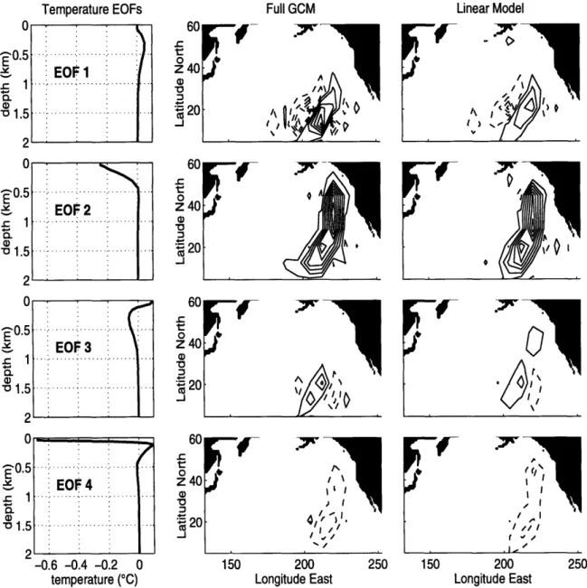
2.2 Vertical EOFs used in linearization of the MIT GCM, and example of propagation of perturbations through the full GCM and the linearized GCM 38

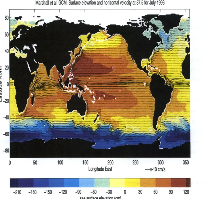
2.3 July monthly-mean sea surface elevation and horizontal velocity in the 2nd

layer produced by the MIT GCM run. . . . . 40

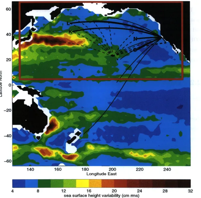
2.4 SSH variability from the T/P and acoustic rays used in the analysis . . . 42

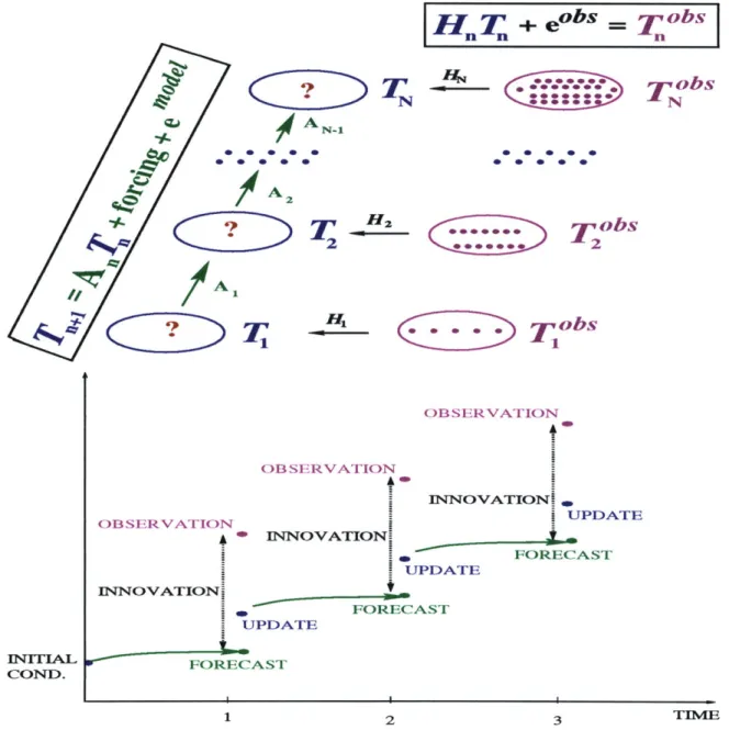
2.5 Scheme of the Kalman filter . . . . 49

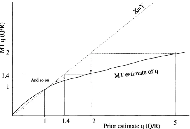
2.6 A graphical representation of the MT adaptive algorithm . . . . 60 2.7 Contour plots of the adaptive estimate of Q/R for 1 DOF model . . . . . 61 2.8 Contour plots of the adaptive estimate of Q/R for 1 DOF model without

(11)

2.9 Example of the estimates obtained with the MT adaptive algorithm with

2 DOF model and 2 observations . . . . 68

2.10 Example of the estimates obtained with the MT adaptive algorithm with

2 DOF model and 1 observation . . . . 70

2 DOF model and 1 observation and only 1 parameter estimated . . . . . 72

2.17 Schematic representation of the twin experiment . . . . 80 2.18 Time series for MT estimates with different observation networks . . . . 91

4.1 Mean diagonal values of sample covariance matrices Y, D1, and D2, as a

function of years of simulated data . . . 128

4.2 _{Estimates of system error variance based on the lag-1 difference sample}

covariance, D1, for simulated acoustic tomography data . . . 129

4.3 Estimates of system error variance based on the diagonal elements of Di

for simulated altimeter data . . . 132 4.4 North Pacific sea level anomaly variance for a) GCM output, b)

TOPEX-POSEIDON data, and c) GCM-TOPEX/TOPEX-POSEIDON residual . . . 134

4.5 _{Prior estimate for percent variance of GCM-TOPEX/POSEIDON residual}

(12)

4.6 GCM-ATOC residual, along the five sections shown on Fig. 2.4 . . . . 139

4.7 Vertical structure of the errors along the ATOC sections . . . . 140

4.8 Trend in the GCM-TOPEX/POSEIDON residual . . . . 141

4.9 Annual cycle peak amplitude for a) GCM output, b) TOPEX/POSEIDON

data, and c) GCM-TOPEX/POSEIDON residual . . . . 142

4 .9 . . . . 143

5.1 Spatial distribution of the variance of the data error in cm2 _{for a) R}

obtained from equation (5.11) and b) R used in F99 . . . . 154

5.2 Variance of the projection of the model error onto the sea level in cm2

(diag HPHT) a) from equation (5.10) and b) for the

Q

used in F99 . . . 155

5.3 Variance of the NCEP wind stress (from F99) . . . . 156

5.4 Relative ratio of the model and measurement errors for the covariance

model used by F99 ... ... 158

5.5 Variance of the residual between T/P data and the GCM simulation . . . 160 5.6 RMS differences of the model-data residuals for the data assimilation done

in F99 ... ... 162

5.7 Estimate of the point cross-covariance between H p and H CGCM,r ' ' * " " 163

5.8 Relative ratio of the model and measurement errors for the rescaled

co-variance model used by F99 . . . . 164

5.9 Sea level anomaly (cm) associated with Kalman filter changes in model

state corresponding to an instantaneous 1 cm model-data difference for

the rescaled and original covariances . . . . 167

5.10 Differences of model-data residuals . . . . 169 5.11 Difference between the variance of the innovations (data-forecast residual)

for the run of F99 and the run with the rescaled error covariances of F99 171

5.12 Sea level anomaly associated with Kalman filter changes in model state

corresponding to an instantaneous 1 cm model-data difference for a new

(13)

5.13 Difference (in cm) between the variance of the innovations (data-forecast

residual) for the run of F99 and the run with the new parametrization of the error covariances . . . 175 5.14 Differences of model-data residuals with the new parametrization for the

error covariances . . . 176

5.15 Contributions to the model error variance from different model variables 179 5.16 Contributions to the model error variance from different model variables 180 B.1 Graph of g(q), A = A = 0.9 . . . . 194 B.2 A plot of g(d; A, A, 4, 1) - 4 for A . . . 196

(14)

List of Tables

2.1 Estimates of the parameters defining the model error covariance for single

application of the MT algorithm with simulated altimetric measurements 82

2.2 Estimates of the parameters defining the model error covariance for single

2.3 Estimates of the parameters defining the model error covariance for single

application of the MT algorithm with observations of all DOF . . . . 87

2.4 Estimates of the parameters defining the model error covariance for sin-gle application of the MT algorithm with simulated acoustic tomography

m easurem ents . . . . 88

2.5 Estimates of the parameters defining the model error covariance for single

4.1 Estimates of system error covariance matrix

Q

based on 14 months of

simulated acoustic tomography data . . . . 130

4.2 Estimates of system and measurement error variance based on 14 months

of simulated acoustic tomography data with R = I . . . . 131

4.3 Estimates of system error covariance matrix

Q

based on 48 months of

perfect, R = 0, simulated altimeter data . . . . 133

A.1 Summary of notation . . . . 189 A.1 ... .... ... 190 A .1 . . . . 19 1

(15)

A.2 Summary of abbreviations . . . 192

F.1 Number of elements of the covariance matrix R, depending on the inputs into covdiff.m or covcov.m . . . 205

(16)

Chapter 1 Introduction

1.1 Data Assimilation in Oceanography

In recent years it has become clear that to understand human induced climate change we first need to understand the natural variability of the world climate. The world ocean is one of the parts of the climate system which we understand least. The spatial scales of the large scale ocean circulation are grand, and the intrinsic time scales are very long. To date, the dynamics of this enormous physical system have been grossly undersampled. Observations in the ocean are very difficult and very expensive to make. Laboratory ex-periments are useful, but limited to idealized problems. General circulation ocean models (GCMs) provide numerical solutions to the physically relevant set of partial differential equations (PDEs). They are routinely used to study ocean dynamics. However, GCMs are very complicated and often have to be run at very coarse spatial and temporal reso-lution. The models are imperfect as the equations are discretized, the forcing fields are noisy, the parameterization of sub-grid scale physics is poorly known, etc. Therefore, to study the dynamics one needs to combine models and observations, in what is known as data assimilation, or inverse modeling. The subject of inverse modeling deals with var-ious techniques for solving under-determined problems, and is well established in many fields, e.g. solid-earth geophysics. Wunsch (1996) provides a general treatment of the

(17)

inverse theory applicable to the oceanographic problems.

The process of data assimilation can be viewed from two different perspectives. On the one hand, it filters the data by retaining only that part which is consistent with a chosen physical model. This is a "filter" in the sense of more familiar frequency filters, e.g. low-pass filters which eliminate high frequency oscillations. On the other hand, it constrains the model by requiring that the state of the model is in agreement with the observations. That is, we use the data as constraints for the models and then use the model to provide information about the regions, or fields, for which we have no observations.

In oceanography data assimilation has three main objectives, as described in detail in an overview of Malanotte-Rizzoli and Tziperman (1996). Using data assimilation for dynamical interpolation/extrapolation to propagate information to regions and times which are void of data has been one the primary goals of inverse modeling in oceanog-raphy. For example, the TOPEX/POSEIDON altimeter measures the height of the sea surface relative to the geoid. Using data assimilation, altimetric data can be used to constrain an ocean GCM, and then the output of the GCM provides information about

the dynamics of the ocean interior, e.g. Stammer and Wunsch (1996). By using a

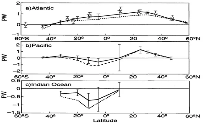
model to extrapolate sea surface height measurements into temperature one can esti-mate meridional heat transport across various latitudes, see Figure 1.1 reproduced from Stammer et al. (1997). Traditionally, one would require sending a ship measuring tem-perature and density profiles across the ocean at all those locations, e.g. Macdonald and Wunsch (1996). Macdonald and Wunsch (1996) used hydrographic data to obtain such estimates at several latitudes where zonal sections were available, shown as open circles on Figure 1.1a. By combining dynamical models with observations one can obtain a global time-dependent picture of the ocean circulation.

In contrast to altimetric measurements which provide information about the sea sur-face, acoustic tomography samples the ocean interior by transmitting sound pulses from a source to a receiver along multiple paths, Munk et al. (1995). To first order, the sound

(18)

2 a)Atlantic 1 ,-609S 40Q 20Q O2 20 40LD 609N 2 - b)Pacific --1

-602S 4 02 00 20 402 609N 0.5 c)Indian Ocean 0 -0. 5 ---1.5 602S 409 202 O0 20 4 0 60 2N Latitude

Figure 1.1: Meridional heat transport (in 1015_{W) for July-December 1993 estimated}

from global data assimilation with the MIT model and T/P data (solid lines). The unconstrained model for the Atlantic, the Pacific and the Indian Ocean respectively, are shown with the dashed lines. Bars on the solid lines show RMS variability of the transport estimated over individual 10-day periods (reproduced from Stammer et al. 1997). speed depends on temperature along the path of the acoustic ray. This temperature information can be then inverted to obtain velocities, displacements, or other physi-cal quantities which can also be estimated from the model output, e.g. Menemenlis et al. (1997b). An example of this is shown on Figure 1.2, where an estimate of depth-averaged temperature and horizontal velocity at a particular vertical level were obtained for the western Mediterranean during beginning of spring, summer and autumn of 1994. Thus, in principle a GCM can be used to extrapolate tomographic data to other areas of the global ocean.

Thirdly, data assimilation can also be used to study dynamical processes by way of improving our understanding of ocean models. Even the most complex ocean GCMs cannot resolve all the dynamically important physical processes, and some processes

(19)

44 13.5 43 20 cm/s 20cm/s 2 42 . .41 38. 13.1 37 13 36 0 2 4 6 8 0 2 4 6 8 0 2 4 6 8 *C

Longitude East Longitude East Longitude East

Figure 1.2: Estimates of the western Mediterranean circulation, on March 1, June 1, and September 1, 1994 obtained by combining tomographic and altimetric observations with a

GCM. The grey scale shading indicates depth-averaged (0-2000m) potential temperature

and the arrows indicate horizontal velocity at 40m (reproduced from Menemenlis et al.

1997).

have to be parameterized. These parameterizations can be simple or quite complex, but are always uncertain in both form and in value of parameters. A few examples of such parameterizations are small scale vertical mixing schemes in the boundary layer, Large et al. (1994), parameterizations of mesoscale eddies in coarse ocean models, Boning et al., (1995), and deep water formation, Visbeck et al. (1996). Observations of most of the above unknown parameters are not available, and many of these parameters cannot be measured directly. They instead can be estimated by using other available data through data assimilation.

Data assimilation can be used for prediction by providing the best estimate of the initial conditions, which are then propagated forward by a model. Forecasting the oceanic fields has become much more important in recent years, and is now done for ENSO on a routine basis. The importance of good initialization fields is clear from a much publicized failure of the Zebiak and Cane model (1987), in predicting the El Ninio event of 1997,

(20)

LAMONT MODEL FORECAST OF NINO3 LDEO 2 LDEO 3 3-.c I-ONDJFMAMJJASONDJFMAMJJASONDJFM ONDJFMAMJJASOHDJFMAMJJASONDJFM 97 98 go 97 9a 99 TIME

Figure 1.3: Lamont model forecasts of the 1997/1998 El Niio with (right) or without (left) sea level data assimilation. The thick curve is observed NINO3 SST anomaly. Each curve is the trajectory of a 12 month forecast starting from the middle of each month. (reproduced from Chen et al. 1998)

e.g. Kerr (1998). Recent analysis showed that with a different data assimilation scheme, and accordingly a different initial field, the model did a much better job of predicting that year's ENSO event, Chen et al. (1998). Figure 1.3 shows striking difference between two groups, LDEO2 and LDEO3, of Zebiak and Cane model, 12 month forecasts. The positive impact of the sea level data assimilation used in LDEO3 but not in LDEO2 is obvious.

While the theory of inverse modeling, including error estimation, has been well devel-oped by the control engineering community, applying it to oceanographic problems is still a challenge. There are at least three major obstacles: computational burden, memory requirements, and lack of required information. That is, problems encountered in control

(21)

series measurements of most, if not all, degrees of freedom. The problems encountered in oceanography tend to be of the opposite nature, i.e. very large number of degrees of freedom, and very short and spatially sparse time series of observations. This difference in the problem size and the amount of available data makes "adoption" of engineering methods to oceanography a difficult exercise. Many properties of the estimation algo-rithms change when observations become sparse and a few, e.g. adaptive Kalman filter

algorithms fail to converge, see Chapter 2.

On the other hand, numerical weather prediction, which is based on data assimilation, has served as a role model for oceanographic data. Although there are clear differences between the ocean and atmosphere, most often applications are similar enough to allow use of similar assimilation methods, and the methods and the literature are common. The reason why the application to the ocean trails has been the lack of urgent demand for forecasting and the lack of appropriate synoptic data sets. However, both of these reasons have recently changed. Oceanic forecasting is being done, and synoptic satellite data sets have become available. As shown in this work, although one needs to be aware of the rich meteorologic data assimilation literature, not all methods can be applied to oceanography, and one needs to develop new techniques more directly relevant to oceanographic problems.

Depending on the temporal and spatial scales of interest, and the computational re-sources available (CPU and memory), one may choose different data assimilation meth-ods, e.g. nudging, adjoint, or Kalman filtering. Typically, for data assimilation with high resolution models one uses the so-called "optimal interpolation" or nudging techniques. The main reason for this is that they are relatively inexpensive from the computational viewpoint. Their main disadvantage is that the choice of weights for blending data and model estimates is chosen in some ad hoc fashion. In a least-squares sense, the optimal solution is given by the Kalman filter (KF, hereafter), Kalman (1960), and a smoother, Rauch et al. (1965). The computational cost of the KF, where one propagates state error covariances at every time step and uses them for estimating the blending weights is great.

(22)

Because of this the KF is currently limited to coarse GCMs and problems where one can significantly reduce number of degrees of freedom.

The KF provides a sequential estimate of the state of the system using only prior information. The estimate is obtained by forming a linear combination of the model forecast and observations, weighted by their corresponding uncertainty. For linear mod-els, the KF, with the companion smoother, is equivalent to the adjoint method. The original KF can be extended to non-linear models, in a so-called extended KF.

The Kalman filter propagates the error covariance matrix, i.e. it provides the accu-racy of the estimate at every time step. Because of this, the KF is very computationally expensive. For a system with n degrees of freedom (DOF, hereafter), 2n + 1 integrations of the numerical model are required for a single time step of the KF algorithm. For systems with a large number of DOF (grid points times number of prognostic variables), at least O(10) for oceanographic applications, this becomes prohibitively expensive even

with largest supercomputers. In addition, the size of the covariance matrices is 0(n 2_),

so that their storage becomes prohibitive as well. To reduce computational and memory costs, many suboptimal schemes have been developed. One can reduce the computational burden by computing approximate error covariances: either by using approximate dy-namics, Dee (1991); computing asymptotically constant error covariances, Fukumori et al. (1993); or propagating only the leading eigenvectors of the error covariances (empirical orthogonal functions, EOFs) as in error subspace state estimation, Lermuisaux (1997).

An alternative way of reducing the computational load is to reduce the dimensionality of the problem. One can reduce the dimension of the model by linearizing a GCM onto a coarser horizontal grid or a small set of horizontal EOFs, and reducing the number of points in the vertical by projecting the model onto a small set of vertical basis functions (EOFs or barotropic and baroclinic modes). For example, Fukumori and Malanotte-Rizzoli (1995) used vertical dynamic modes and horizontal EOFs for their coarse model.

A more detailed explanation of this approach is given in Section 2.1. In a different

(23)

coefficients for each individual EOF, e.g. Cane et al. (1996), Malanotte-Rizzoli and Levin (1999). Although the analysis of Cane et al. (1996) deals with the small domain in the tropical Pacific and only several tide gauges are used, the results suggest that reduced space assimilation is in general not inferior to full Kalman filter for short times, even though the dimension of the model is reduced by several orders of magnitude.

In this work, questions of a more theoretical nature are addressed, namely how to do data assimilation when some of the required input information is absent, e.g. statistics of the errors, as explained below. Therefore, we will concentrate on the basic setup and treat only linearized models. Because for linear models the Kalman filter is the most general data assimilation method, for the purposes of this discussion many other data assimilation methods can be viewed as its special cases, and are not considered.

1.2 Adaptive Error Estimation

Apart from the difficulties associated with the large dimensionality of the problem, it is critical for the statistics of the model errors and the measurement noise to be known for the KF estimates to be optimal. Although in some cases of oceanographic interest the errors in observations may be relatively well-determined, e.g. Hogg (1996), this is not typically true because the measurement errors, as defined in the data assimilation context,include the missing model physics, or representation error. This is due to the fact that the model cannot distinguish the processes which are missing from the model, e.g. scales smaller than the model grid size, from the errors in the observations, see the discussion in Section 2.2. The model errors, or system noise, are usually poorly known.

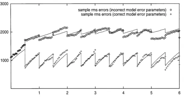
Therefore, the resulting estimate of the assimilated ocean state is far from optimal. Figure 1.4 taken from Dee (1995) shows an example of the effect of incorrectly specified model error statistics on the performance of the KF. The plot shows the time evolution of the root-mean-square (RMS) energy errors for two data assimilation experiments, per-formed with the two-dimensional linear shallow water model of Cohn and Parrish (1991).

(24)

3000

2000

-1000

+ + +

1 2 3 4 5 6

Figure 1.4: RMS energy error evolution for SKF with incorrectly specified (upper part) and correctly specified (lower part) model error statistics. Marks indicate actual RMS errors, curves correspond to their statistical expectations, the time is in days (reproduced from Dee 1995) .

The curves correspond to statistical expectations of forecast and analysis errors obtained from KF theory while the marks denote the errors that actually occurred. In each exper-iment the same 12-hourly batches of synthetic radiosonde observations were assimilated into a forecast model by means of a simplified KF (SKF), Dee (1991). The two experi-ments differ only in the way that the model error covariance is specified. The RMS-error curve and marks in the lower part of the figure result from a correct specification of model error covariance, while those in the upper part result from a misspecification of the model error covariance. The disastrous effect of erroneous model error information is clearly visible. The average analysis error level more than doubles after a few days of assimilation. In some cases the assimilation of observations actually has a negative impact on the analysis (e.g. days 0.5, 1.5, and 5.5).

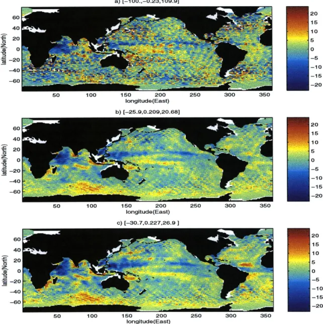
In Figure 1.5 we demonstrate the effect of error covariances on the estimates of the ocean state. The figure shows a comparison of the sea surface height anomaly for one particular cycle of the T/P altimeter (January 1-10, 1994). The top plot shows the

(25)

T/P measurements, and the two lower ones show corresponding estimates obtained us-ing the T/P measurements with an approximate Kalman Filter (Chapter 5)1. It has to be noted that these data assimilation experiments were done with carefully chosen, and not very different, error covariances. The small-scale signal seen in the T/P measure-ments is missing in the KF estimates because the assimilation was done with a coarse grid (reduced-state) model, i.e the KF serves as a filter to remove the small scales. Be-cause the error covariances were similar, the two fields obtained with the KF are similar overall. However, there are important differences. For example, the second assimilation (Figure 1.5c) has a strong positive anomaly in the West Equatorial Atlantic which is completely missing in the first assimilation. Unlike the twin experiment example pre-sented above, in this case we do not know the true state. Although there are some tests which allow to check consistency of the estimates, it has been shown that application of such tests to global data assimilation with realistic data distribution is problematic (Daley, 1993). Unless one has independent data, it is difficult to decide which of the two estimates is "better", i.e. closer to the true field. Only careful choice of the a priori error covariances can make the estimates of the state credible.

To make matters worse, when we have wrong estimates of the error covariances, the estimates of the state uncertainty are also wrong, i.e. both estimates of the state and its uncertainty depend critically on the covariances of the model and measurement errors. In addition, the state itself depends on the first-order moments, or bias, of the errors.

Error covariances are also very useful for analyzing the performance of a GCM. They provide information on which geographic locations and what spatial scales the GCM's performance is good or bad. In addition, they set a metric for comparing different GCMs.

A quantitative tool which would allow one to perform such comparisons would be highly

desirable, for an example of the difficulties one faces when attempting to evaluate the performance of different atmospheric GCMs see Gates (1995).

1_{The data assimilation estimates have used 1 year of the T/P measurements starting from January}

(26)

a) [-100.,-0.23,109.9] 20 -20 40 2 220 0 15 ) -0 5 Id -20 -10 -60 -20 50 100 150 200 250 300 350 longitude(East) b) [-25.9,0.209,20.68] eO0 40 5 20 -20 -220 VC -10 -40 -60 -20 50 100 150 200 250 300 350 longitude(East) c) [-30.7,0.227,26.9] 60 40 S20 -20 -40 -20 so 150 10 200 50 30 10

Figure 1.5: Sea surface height anomalies (in cm) for the a) T/P data set, b) and c) data assimilation estimates using the same T/P observations for two different choices of the error covariances. The error covariances for the data assimilation were chosen adaptively (Chapter 5), and were not very different. Overall, the two assimilation estimates are Sim-ilar, but there are significant differences, e.g. in the equatorial Atlantic. The assimilation runs are described in Chapter 5.

(27)

1.3 Present Work

The problem of estimating and understanding the error statistics is the subject of this work. It has only recently received attention in the oceanographic community. For a long time the problem did not attract significant attention for several reasons. First, use of the error statistics requires a very significant increase in computational resources, and a significant reduction in the number of degrees of freedom. The methods of state reduction, see Chapter 2, have not been tested and applied to large GCMs until recently. In addition, one needs to use approximate data assimilation schemes, and they also have only recently been developed. Thirdly, the fact that the estimation is sensitive to the specification of the statistics of the observational, and especially model errors, needed to be established, e.g. Wergen (1992). It is worth noting that operational centers still routinely use a "perfect model" assumption, even though there is a strong consensus that present-day GCMs have great difficulty in simulating the real ocean and atmosphere.

The following is a sequential account of the work which can be taken by someone who faces the problem of estimating error statistics for large-scale data assimilation and who wants to understand why the covariance matching algorithm (CMA, hereafter) was developed and what are its advantages. Alternative ways of reading the manuscript are discussed below in Section 1.3.1.

We start addressing the error estimation problem by presenting existing adaptive data assimilation methods. In the present context the term "adaptive" means that we are using data for the simultaneous estimation of the error statistics and the ocean's state. Such adaptive methods were applied to an oceanographic problem in a paper by Blanchet et al. (1997), (BFC97, hereafter). BFC97 ran twin experiments with three dif-ferent adaptive data assimilation methods, developed and improved upon by a number of different authors in the control and meteorological literature. BFC97 used simulated tide-gauge data and a reduced-state model in the tropical Pacific. In Chapter 2 we test these adaptive methods by trying to obtain quantitative estimates of the large scale inter-nal errors in a GCM using simulated T/P altimeter data as well as acoustic tomography

(28)

data.

Following the discussion in BFC97 we single out the adaptive method of Myers and Tapley (1976, MT) as the representative of these adaptive methods. Firstly, we present the analysis of the MT method, with low dimensional models. We show that while in principle this method can provide estimates of the model error statistics it has several major drawbacks. When we have sparse observations, the estimates of the error statistics may be sensitive to the initial guess of the model error covariances. The method requires running the Kalman filter, and it takes many iterations for the method to converge. This makes it computationally expensive. Estimation of both model and measurement statistics is unstable, and can lead to wrong estimates. There is no information about uncertainties of the derived error covariances, on how much data is required, and on which parameters can be estimated and which cannot.

We use a twin experiment approach, described in Section 2.8, to show that with the linearized MIT GCM, the MT method is sensitive to the initial choice of the error statistics, and to the kind of observations used in the assimilation. In Section 2.9 we show that similar results are obtained with a maximum likelihood method. The conclusion is that neither of the adaptive data assimilation methods is suitable for quantifying large scale internal ocean model errors with the available altimetric or acoustic tomography observations.

In a different approach, Fu et al. (1993) and Fukumori et al. (1999) estimated the measurement error covariance by comparing the observations with the model forecast without any data assimilation. This method is closely related to the new approach, which we develop and call the Covariance Matching Approach (CMA). It is described in Chapter 3. Although related to the previous methods, the new approach relaxes some of the restrictive assumptions of the method used by Fu et al. (1993). It makes use of information in a more efficient way, allows one to investigate which combination of parameters can be estimated and which cannot, and to estimate the uncertainty of the resulting estimates.

(29)

In Chapter 4 we apply the CMA to the same linearized version of the MIT GCM with ATOC and T/P data. Through a series of twin experiments, which use synthetic acoustic thermometry and T/P data, we show that the covariance matching approach is much better suited than the innovation-based approaches for the problem of estimating internal large scale ocean model error statistics with acoustic measurements, but not with altimetric measurements. Because the method uses observations directly instead of the innovations, it allows concurrent estimation of measurement and model error statistics. This is not possible with the adaptive methods based on innovations (Moghaddamjoo and Kirlin 1993).

We then test the CMA with the real TOPEX/POSEIDON altimetry and the ATOC acoustic tomography data. We show that for this model most of the model-data misfit variance is explained by the model error. The CMA can also be extended to estimate other error statistics. It is used to derive estimates of the trends, annual cycles and phases of the errors. After removal of trends and annual cycles, the low frequency/wavenumber (periods > 2 months, wavelengths > 160) TOPEX/POSEIDON sea level anomaly is

order 6 cm2_{. The GCM explains about 40% of that variance, and the CMA suggests that}

60% of the GCM-TOPEX/POSEIDON residual variance is consistent with the reduced

state dynamical model. The remaining residual variance is attributed to measurement noise and to barotropic and salinity GCM errors which are not represented in the reduced state model. The ATOC array measures significant GCM temperature errors in the

100-1000 m depth range with a maximum of 0.3 at 300 m.

In Chapter 5, we apply the CMA to a second problem, one which involves estimat-ing global ocean error statistics for a linearized GFDL GCM, with only the barotropic

and first baroclinic internal modes2_{. The obtained estimates of error statistics are}

sig-nificantly different from those used in the study of Fukumori et al. (1999), where the 2_{Although the vertical modes can only be defined for the linear ocean model, they can be used as}

a set of vertical basis functions. Fukumori et al. (1998) show that the barotropic and first baroclinic mode explain most the variability of the T/P sea level anomaly. A linearized model based on these two modes is satisfactory for data assimilation needs.

(30)

linearized model is used for global data assimilation. The CMA estimate of the model error covariance based on the error model of Fukumori et al. (1999) on average explains forty percent of the model-data residual variance. Most of the model error variance is explained by the barotropic mode, and that the model error corresponding to baroclinic velocities has a negligible contribution.

The CMA estimates of the error covariances are then used with a global data as-similation scheme. Based on analysis the statistics of the innovations, we show that the quality of the data assimilation estimates is improved very little. As pointed out in Chap-ter 3 the problem of error statistics estimation is very under-deChap-termined. Therefore, to obtain statistically significant estimates of the error statistics it is crucial to have a good physical understanding of the model shortcomings. The covariances used in Fukumori et al. (1999), already tuned to the model-data residuals, use the error structures which prove to be quite robust. Comparison of several data assimilation experiments which differ only

by the choice of the error covariances demonstrate that data assimilation estimates are

not very sensitive to a particular parametrization of the adaptively tuned error statistics. The summary of the thesis and perspectives for future research are given in Chapter 6.

1.3.1 Outline of the Thesis

With a complete description of the work given above, we give advice on how to read the thesis. A complete summary of the notation (with a reference to the original equations) and acronyms is given in tables A.1 and A.2.

The reader who is primarily interested in the results can start directly with the examples. An application of the CMA to a linearized version of the MIT GCM with the

TOPEX/POSEIDON altimetry and the ATOC acoustic tomography data is presented

in Chapter 4. Second application of the method and an example of data assimilation with adaptively tuned error covariances are presented in Chapter 5. The model used in this chapter is a linearization of the global GFDL GCM and the data consist of the T/P measurements of sea level anomaly.

(31)

For a more detailed description of the CMA the reader should consult Chapter 3. The basic algorithm is presented in Section 3.2. For a discussion of practical issues which are important in realistic applications and for the extensions of the method to other statistics one should consult Sections 3.3 and 3.5.

For a reader familiar with, or interested in, innovation based adaptive methods, a comparison of innovation based methods and the CMA is presented in Section 3.6. To get a deeper understanding of an innovation-based approach due to Myers and Tapley (1976), one can consult Section 2.6, where an analytical representation of the method with a scalar model is discussed, and Section 2.7, where a numerical implementation of the method with a multivariate (2 DOF) model is given. In Section 2.8 we demonstrate that this method fails with a linearized version of the MIT GCM, while the CMA can be successfully used in the same setup presented, Section 4.3.

The reader who is willing to take the time and travel the long road can read the work sequentially as described above.

(32)

Chapter 2 Methods of Adaptive Error

Estimation

We start this chapter by setting the problem up and providing a mathematical descrip-tion. We then discuss available methods of adaptive error estimadescrip-tion. To illustrate the methods we restrict our attention to the following question: "For a linear model with four vertical modes, can we estimate the mean variance of model error for each mode based on the two kinds of available measurements: altimetric measurements of the sea surface height and acoustic tomography measurements of sound speed converted into temperature anomalies?" We use a linearized GCM of the North Pacific, where more than a year of high quality acoustic data are available in addition to the altimetric data. We use the GCM of Marshall et al. (1997a, 1997b) and the reduced state linearization described in Menemenlis and Wunsch (1997). We concentrate on the adaptive method of Myers and Tapley (1976) (MT, hereafter), and in addition consider the maximum likelihood approach of Dee (1991, 1995).

After we describe the model and the methods, we investigate properties of the MT algorithm with low-dimensional systems in order to gain better understanding of the al-gorithm. We start with a model with one degree of freedom, and then extend the results to a model with two degrees of freedom. The analysis with low-dimensional models

(33)

illus-trates the non-linear character and complexity of the adaptive error estimation problem. It provides guidelines for the applicability of the MT algorithm.

Next, we present results of twin experiments with a linearized GCM, i.e. experiments for which synthetic data are used. We start with a series of the experiments in which we compute a single posterior estimate of both model and measurement uncertainties. These runs allow us to sample the parameter space and to develop intuition for the par-ticular linear model appropriate to our experiment and for the two kinds of measurement, altimetric and tomographic. We then present a series of fully adaptive twin experiments. Based on the twin experiments we show that the performance of the adaptive filter de-pends on the type of observations. The adaptive method of MT cannot estimate the correct uncertainty structure with synthetic altimetric observations, but can do so once a significant number of synthetic tomographic rays are included in the assimilation. How-ever, it fails with the tomographic measurements available at the time this analysis was carried out.

Based on these results, and the fact that the method is sensitive to the initial guess of the error covariances, and, moreover, provides no information on the uncertainty of the derived estimates, we conclude that the estimates we would obtain with real data could not be trusted. In addition, we show why the maximum likelihood method of Dee (1995), provides similar negative results (Section 2.9.1).

The chapter is organized as follows. In the next Section we present the model and the observational networks used in this chapter. In Sections 2.4-2.5 we review the basic and adaptive Kalman filter algorithm. For analysis of the MT method with a one degree of freedom (DOF) model for which analytical representation is obtained see Section 2.6. In Section 2.7 we turn to the analysis of the MT adaptive filter with a 2 DOF model, which allows to consider the important case of incomplete data coverage. In Section 2.8 we present the results of the twin experiments with simulated altimetric and acoustic tomography data. We draw conclusions about the performance and limitations of these adaptive techniques in Section 2.10.

(34)

2.1 Model

Dynamical models describe how information, or physical properties, propagate in space and time. Ocean models describe how the physical quantities of the ocean (e.g. fluid velocities, temperature, and pressure) change in time and space. Given boundary and initial conditions, we can use the model to obtain information about the state of the ocean in a particular region of the ocean, or at some later time. For reasons outlined in the introduction we will be concerned only with linear, or linearized, models. Below we provide a short description of how a linearized ocean model can be obtained. Complete descriptions of the two different linearized models used in this work are given by Mene-menlis and Wunsch (1997), for the linearized MIT GCM, and by Fukumori et al. (1999), for the linearized GFDL GCM.

The models are discretizations of the incompressible Navier-Stokes (NS) equations together with an equation of state. The MIT GCM, developed by Marshall et al. (1997a,

1997b), the linearization of which is used in this chapter, solves the NS equations in

spherical geometry with height as a vertical coordinate and with arbitrary basin geometry. It is integrated in hydrostatic mode for the Pacific Ocean with realistic topography and coast lines, and insulating bottom and side walls. A no-slip wall side condition and a free-slip bottom condition are used. The model domain extends from 30 S to 61 N meridionally, and from 123 E to 292 E zonally, with a uniform horizontal grid spacing of 10. There are 20 vertical levels, with a maximum depth of 5302m. The model time step is 1 hour.

The model is relaxed to climatological values of temperature and salinity at the surface with a time scale of 25 days. Because the model is restricted to the northern part of the Pacific, at the southern boundary the model is relaxed over a 500 km zone with a time scale of 5 days at the boundary increasing linearly to 100 days at the edge of the 500 km. To obtain a model for large scale ocean climate estimation studies, we need to linearize

(35)

the model and to reduce its dimension. First, the GCM is represented algebraically as

CGCM(t + 60) [CGCM Wt, WGCM (2.1)

where WGCM(t) represents boundary conditions and model parameters at time t. Column vectors are written as bold lower case characters, and matrices as bold upper case char-acters. A complete summary of the mathematical notation is presented in Table A.1.

The state GCM(t) consists of all prognostic variables used in the GCM, and as such has

dimension of 1,335,582 for the configuration used in computing the linearized model. We make a fundamental assumption that for large scales, the difference between the true state on the model grid and the model state,

p(t) = B*[(GCM) - CGCM(t)], (2.2)

is governed by linear dynamics:

p(t + 1) = A(t)p(t) + P(t)u(t), (2.3)

where p(t) is the coarse state (large scale) error vector, B* defines a mapping from the fine (GCM grid) to the coarse (large scale) grid; A(t) is the coarse state transition matrix; u(t) is the model error vector, and T(t) projects the large scale model error u(t) onto the coarse state. Note that we distinguish the GCM error in the reduced (coarse) space, p(t), from the stochastic noise driving the GCM error, u(t), denoted as model error for consistency with the standard KF notation. The true state is denoted by the circumflex. The time step of the reduced state model has been taken to be unity, and in practice is considerably longer than the time step of the GCM. We use a 30 days time step for the linearized model (LM, hereafter) and one-hour time step for the MIT GCM.

It is important to realize that the linear model is not a linearization of the model around its mean state, such as a commonly used linearization of the non-linear quasi-geostrophic model (Pedlosky, 1987 , p. 499). The linear model, equation (2.3), provides an approximate description of how the large scale differences of the GCM estimate and the true ocean on the GCM grid propagate in time. This assumption is based on a

(36)

fundamental requirement that the large, slow scales of oceanic variability are separated from meso-scale and other short-term variability, and that the smaller scales effect on the large scale differences can be modeled as a white noise process; see Menemenlis and Wunsch (1997).

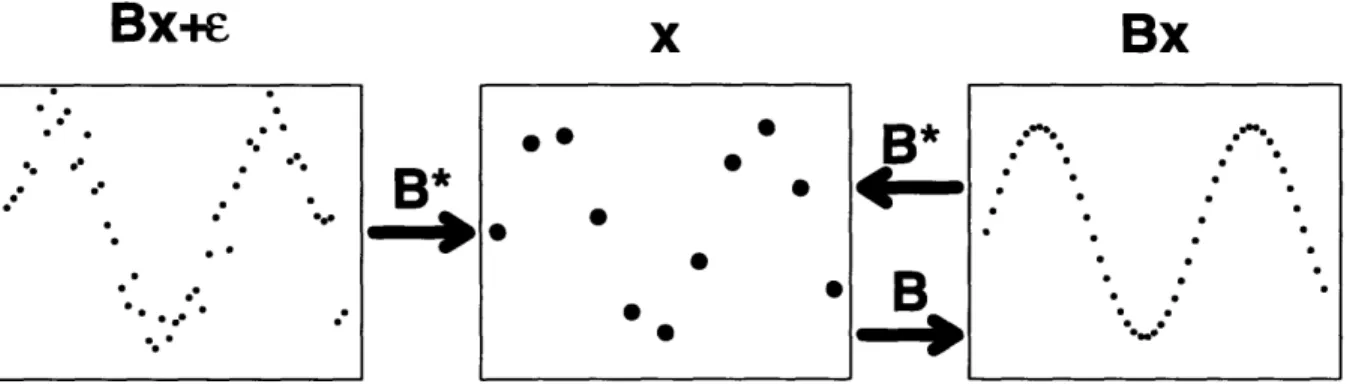
The state reduction operator B* projects the difference between the hypothetical true state and the model state onto some truncated basis set. In practice, the true state

CGCM (t) is approximated by some reference state (, and the linearization is effectively done

around that state; see Fukumori and Malanotte-Rizzoli (1995). The reduction operator may be thought of as a filter which attenuates small scale noise in order to capture the relevant ocean-climate signal. A pseudo-inverse operator, B*, which maps back from the coarse (reduced) state to the fine (GCM) state can be defined such that

B*B = I, BB*

#

I, (2.4)

and I is the identity matrix. Therefore, it is possible to write

Bp(t) + E(t) = [CGCM(t) - CGCM(t))J, (2.5)

where E(t) represents the high frequency/wavenumber components that lie in the null

space of the transformation B*,

B*E(t) = 0, (2.6)

o

is the matrix of zeroes. These operators are represented schematically in Figure 2.1.

The linearized model implies that the large-scale perturbations described by the linearized state vector p(t) are approximately dynamically decoupled from the null space, i.e.

B*M(E(t)) ~ 0. (2.7)

The validity of this assumption needs to be tested with each particular model. We refer the reader to Sections 4 and 6 of Menemenlis and Wunsch (1997), for a demonstration of its validity with the MIT GCM.

(37)

**Bx*w**

x

_Bx

.- . .- e *

4 .

.

_-....

..- --.

B

-

-- .--

0

Figure 2.1: Schematic representation of the interpolation and state reduction operators. The primary purpose of the state reduction operator, B* in (2.2), is to reduce the problem size while preserving sufficient resolution to characterize the important physical processes under study. The choice of B* needs also to be guided by sampling requirements so as to avoid aliasing. One may wish to define B* as a combination of horizontal, vertical, and time reduction operators:

B* = B*B*B* (2.8)

Corresponding pseudo-inverse operators can be defined and

B = BtBvBh. (2.9)

In practice, each pseudo-inverse operator can be defined as

B = B*T (B*B*T)fl, (2.10)

where superscript T denotes the transpose. Non-singularity of B*B*T is satisfied for any but the most unfortunate choice of B* since the number of rows of B* is much less than number of columns. For the linearization of the MIT GCM, the vertical state reduction operator B* maps perturbations onto four vertical temperature EOFs, computed from the difference between GCM output and measured temperature profiles; see Menemenlis et al. (1997a). The EOFs are displayed on Figure 2.2. Horizontal filtering is done using a two-dimensional Fast Fourier Transform algorithm, and setting coefficients corresponding