HAL Id: hal-01360390
https://hal.archives-ouvertes.fr/hal-01360390
Submitted on 5 Sep 2016
HAL is a multi-disciplinary open access
archive for the deposit and dissemination of
sci-entific research documents, whether they are
pub-lished or not. The documents may come from
teaching and research institutions in France or
abroad, or from public or private research centers.
L’archive ouverte pluridisciplinaire HAL, est
destinée au dépôt et à la diffusion de documents
scientifiques de niveau recherche, publiés ou non,
émanant des établissements d’enseignement et de
recherche français ou étrangers, des laboratoires
publics ou privés.
Rate of chaotic mixing in localized flows
Jalila Boujlel, Franck Pigeonneau, Emmanuelle Gouillart, Pierre Jop
To cite this version:
Jalila Boujlel, Franck Pigeonneau, Emmanuelle Gouillart, Pierre Jop. Rate of chaotic mixing in
localized flows.
Physical Review Fluids, American Physical Society, 2016, 1 (3), pp.031301(R).
�10.1103/PhysRevFluids.1.031301�. �hal-01360390�
protocol with a rotating vessel. Only a limited zone localized around the stirring rods is highly sheared at a given time. Using a dyed spot as initial condition, we measure the decay of concentration fluctuations of dye as mixing proceeds. The mixing rate is found to be proportional to the volume of highly-sheared fluid during a rotation period of the rods, and inversely proportional to the number of rotations of the rods over a rotation of the vessel. Thanks to numerical simulations and experimental measurements, we relate the volume of highly-sheared fluid to the parameters of the flow. We propose a quantitative two-zone model for the mixing rate taking into account the geometry of the highly-sheared zone, as well as the rate at which fluid is renewed inside this zone. For all experiments, the model predicts correctly the scaling of the exponential mixing rates during a first rapid stage, and a second slower one.
Chaotic advection [1] is a preferred physical mecha-nism for mixing fluids at low Reynolds number. The stretching and folding of fluid filaments results in an ex-ponential separation of neighboring particles with time, and in a fast mixing rate compared to diffusion alone, as characterized for example by the decay of concentration fluctuations [2–7]. Fluctuations decrease when concen-tration heterogeneities are stretched into thin filaments, down to an equilibrium diffusion scale at which molecular diffusion blurs filaments together [6].
An important fundamental and practical challenge consists in understanding and predicting the mixing rate from the geometrical and rheological parameters of the mixing flow. Theoretical studies [2–4, 8, 9] suggested that large-deviation statistics of the distribution of stretch-ing factors of trajectories determine the long-time mix-ing rate, and numerical experiments on ideal simplified flows [4, 10, 11] confirmed the validity of such models for some cases. However, relating quantitatively kine-matic flow parameters to the distribution of stretching factors, or its statistics, is hard to achieve. No such at-tempt has yet been made in the mixing literature for a realistic mixing flow, with the noteworthy exception of flows for which successive stretching factors are uncorre-lated enough that stochastic models of random convolu-tion account well for mixing rates as well as concentraconvolu-tion distributions [5–7, 12]. Such cases include flow in porous media [13] or turbulent flows [5]
In this work, we consider an experimental mixing de-vice in which the shearing and stretching of fluid particles is strongly localized around mobile obstacles, so that the distribution of stretching is simple enough that two zones can be defined: one close to the moving cylinders where the shear is high and the other part which experiences only small shear. This enables to predict analytically the mixing rate from flow parameters. For this purpose, we study the mixing of non-Newtonian viscoplastic fluids, that start to flow only when submitted to a stress larger
than a critical value, called yield stress. This behavior affects the mixing performance, due to shear localization that can in the worst case generate dead zones inside the mixing device [14–16]. Since mixing yield-stress fluids is an operation involved in several industries such as cos-metic, polymer, petrochemical, pharmaceutical, or food engineering [16–18], an abundant literature in engineer-ing [14–17, 19] has focused on design and upscalengineer-ing of flows in order to reduce such dead zones. A few stud-ies have addressed the description of chaotic advection in flows of viscoplastic [20–22] or other types [23, 24] of shear-thinning fluids, demonstrating in particular the the shear localization is often responsible for a very scattered distribution of stretching factors [21].
The main goal of this study on viscoplastic fluids is to relate the mixing rate to experimental parameters that govern it, in particular to evaluate the impact of the rhe-ological properties of the fluid and the geometry of the device on the mixing process. To this end, we character-ize experimentally the mixing rate in a two-dimensional flow with chaotic advection. We study the mixing of a transparent yield-stress fluid with a blob of the same fluid dyed with black ink (Pebeo). We use the same setup as described in [22]. The device (Fig.1.a) consists of two pairs of cylindrical stirring rods, counter-rotating with a constant angular velocity on circular trajectories. The outer cylindrical vessel is also rotating. We define the ratio S = Tvessel/Trods, between the period of rotation of
the vessel and the period of rotation of the rods. As yield stress fluids we use solutions of Carbopol EZ3 in water at different concentrations [25]. We verified that their flow curve, i.e. the steady-state shear stress (τ ) as a function of the shear rate ( ˙γ), is well fitted by a Herschel-Bulkley model, τ = τc+ k ˙γn, where τc is the yield stress and k
and n are material parameters [26]. Since we found con-stant values for n ' 0.33 and τc/k ' 1 for all polymer
concentrations, in the following we describe the materials only through their yield stress value τc.
2
FIG. 1. (a) Typical images obtained at different times of mix-ing. (b) and (c) Evolution of the variance of the concentration of the dye with time, for different rod diameters d (τc= 27 Pa) (b) and for different values of yield stress τc(d = 7 mm) (c). The vertical dashed line on graph (c) separates the two mixing regimes.
To quantify the mixing process, we follow the evolu-tion of the dye concentraevolu-tion field during the experiment by taking photographs through the transparent bottom of the mixing vessel, once per rotation period of the rods. A blob of dyed fluid is released in a plane at mid-height of the vessel, inside the central zone of the vessel sec-tion (Fig.1.a left). The eggbeater-like mosec-tion of the rods as well as the rotation of the vessel promote efficient chaotic advection through stretching and folding of fluid filaments (Fig.1.a center), so that no non-chaotic islands are observed in the center of the vessel, which would have led to the formation of either dye free zone or persis-tent dye blob. Nevertheless, a non-chaotic dye-free zone (Fig.1.a center and right) exists close to the boundary of the vessel, consisting of fluid that is entrained in solid rotation for most of the vessel period – it is only sheared when stirring rods pass close-by. During the first periods of mixing, the initial blob of dyed fluid (Fig.1.a left) is stretched into many filaments that quickly fill the chaotic region (Fig.1.a center); the asymptotic mixing pattern (Fig.1.a right) consists of the chaotic region delineated by the dyed fluid, and the dye-free non-chaotic region.
The standard deviation of the dye concentration inside the mixing region is determined by image processing, us-ing Beer-Lambert law for light absorption. We normalize the measured value of the standard deviation by the av-erage value of the asymptotic concentration inside the mixing region, so that this value σC is independent of
the amount of dye injected in different experiments. The evolution of the variance with the number of rotation periods of the rods shows the existence of two distinct mixing regimes (Fig.1 b and c). First, exponential decay occurs when dye filaments are stretched by the rods,
un-(c) (a)
(e) u/U Solid
0 x U (d) 6 s 20 s 45 s Trods (b) Cylinder Liquid :
FIG. 2. (a, b, c) Pictures of mixing showing the dependence of the thickness of the dye filament formed behind the rod (red arrow), on the rod diameter: (a) d = 3 mm ,(b) d = 7 mm and (c) d = 15 mm, for Trods= 6 s. (d) Influence of the speed of the rod on the thickness of the dye filament (d = 7 mm), after the first period for Trods= 6 s, Trods= 20 s and Trods = 45 s. (e) Schematic of the morphology of the flow around a cylinder moving at constant speed through a yield stress fluid, highlighting the boundary layer and the area of thickness δ0, where the shear is very intense and localised near the cylinder (case of low values of Bi).
til their width reaches in turn the Batchelor scale [5], at which molecular diffusion balances stretching and smears out concentration fluctuations (as in Fig.1.a center). At the end of this regime, dye filaments almost fill the en-tire chaotic region. Then, a slower mixing regime, also exponential, occurs when remaining fluctuations are due to the slow transport of fluid from the periphery of the chaotic region (where stretching is typically lower) to the core of the chaotic region. This can be observed in Fig.1.a.right as funnels of dye-free fluid originate from the boundary of the mixing pattern, and result in fila-ments of fluid injected inside the mixing region with a different (lower) concentration level. In this final regime, the mixing rate is controlled by slow transport between a zone of low stretching (here, the periphery) and a zone of high stretching (the core). The resulting structured pattern of funnels of dye-free fluid being stretched into thin filaments is the so-called strange eigenmode [27], a persistent pattern that corresponds to the slowest decay-ing eigenmode of the advection-diffusion operator [28– 30]. We characterize the mixing rate by the exponential rates of the first and second regimes, λ1 and λ2:
σC2(t) ∝ exp (−λ1,2t/Trods) . (1)
In order to identify the mechanisms and key parame-ters that control the mixing process, we study the vari-ation of the mixing rate with the diameter d and the velocity of the rods U , the stirring ratio S, and the yield
range that we tested (Fig.1.c).
Flow around a rod - When a stirring rod first passes through the dyed blob, the thickness – hence the amount – of dyed fluid stretched and carried away by the rod in-creases significantly with the diameter of the rod (Fig.2.a, b, c.) or its speed (Fig.2.d.). As we will elaborate on later, the enhanced transport and stretching of fluid re-sult in faster mixing. Let us first estimate the volume of fluid stretched efficiently by one rod during a period of ro-tation. We consider the flow generated around a cylinder moving at constant velocity through a yield-stress fluid. Because of the viscoplasticity of the fluid, the flow will be strongly localized around the rods. According to the lit-erature [31–33], there exists a limited sheared and liquid region around the cylinder, while the rest of the mate-rial is negligibly deformed and can be considered solid (Fig.2.e). Furthermore, it has been shown [33–35] for Bingham fluids [36] that the shear is very localized and very intense within a thin boundary layer close to the cylinder (see the schematic velocity profile in Fig.2.e). We note δ0 the typical thickness of this boundary layer.
While the shear is very intense inside the boundary layer, the rest of the fluid of the liquid region is only weakly sheared. This thin boundary layer is therefore a good candidate to characterize the volume of fluid efficiently stretched by the rods.
Dimensional analysis suggests that the size of the boundary layer depends on the rod diameter d and on the Bingham number Bi, which is the ratio of yield stress to viscous stress. For a Herschel-Bulkley fluid, the Bingham number is defined as Bi = τc
k( d U)
n. For Bingham fluids,
Tokpavi et al. [35] showed numerically that δ0 can be
expressed as δ0 ∝ d Bi−0.54, for a Bingham number Bi
ranging from 10 to 2.105. Since no information exists in
the literature about the size of the boundary layer for a Herschel-Bulkley fluid, we performed numerical simula-tions.
To evaluated the thickness of the shear layer around a cylinder numerically, we choose the configuration of a moving 2D cylinder of diameter d in a straight channel of width w = 4d at constant velocity U . The fluid is a Herschel-Bulkley fluid whose shear stress σ is given by σ = τc+k ˙γn, where τcis the yield stress, k and n are
ma-terial dependent. We set the same value for the exponent n as in experiments (n = 0.33) and the dimensionless mo-mentum equation simulated are scaled by the Bingham number. Numerical simulations are performed using the finite-element library Rheolef [37]. Using the augmented Lagrangian method and a mixed finite-element method [38], we computed the steady velocity profile and derive the value of δ0 by extrapolating to zero the lateral
ve-(0.48 + Bi1.3)0.53
The form of the equation is chosen to provide a good agreement of the data while keeping a compact form. The figure 3 shows the results of the simulations and the fit by equation 2.
FIG. 3. Thickness δ of the strongly sheared layer around a cylinder moving in a Herschel-Bulkley fluid at constant veloc-ity (•). The line is a fit following the equation 2 Inset: The residuals are lower than 2% in the range of interest of the experiemnts.
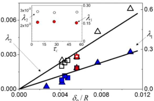
FIG. 4. Mixing rates λ1 (full symbol) and λ2(empty symbol) versus δ0/R (computed from Eq. 2), with d ∈ {3, 5, 7, 10, 15} mm (triangles), Trods ∈ {6, 20, 30, 45} s (square) and τc ∈ {7, 27, 54} Pa (circles), and at constant stirring ratio S = 5.5. The lines are fits forced through the origin. Inset: Same data only related to the impact of the yield stress, highlighting the constant values of λ1 and λ2, independent of τc.
For the different experiments at constant S, we have represented in Fig.4 the mixing rates, λ1 and λ2,
4 characteristic thickness δ0normalized by the radius of the
area scanned by the rods R (which corresponds roughly to the radius of the chaotic zone, Fig. 1.a.right). For the two regimes, all results collapse on a linear master curve, meaning that δ0is the relevant parameter to capture the
evolution of the mixing rates with the rod speed, the di-ameter, or the yield stress, and that the mixing rate of a yield-stress fluid is controlled by the boundary layer generated around the stirring rod. The good correlation between δ0 and the mixing rates explains the absence of
impact of the yield-stress value on the mixing rate (see inset in Fig. 4). Indeed, δ0 depends via Bi on the ratio
τc/k, that is constant for our different fluids.
Neverthe-less, δ0can be varied in our experiments by using different
rod diameters and velocities.
We now propose a model in order to account for the lin-ear dependence between the mixing rates and δ0. Let us
start by considering λ1, the mixing rate during the first
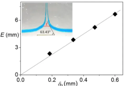
regime. In this two-zone model, we proposed that the part of fluid highly stretched by the rods is that strongly sheared in the boundary layer. We checked this hypoth-esis thanks to complementary experiments where a thin strip of colored fluid was deformed by a cylinder moved at constant speed perpendicularly to the strip. Measure-ments obtained with different cylinder diameters show that the width of the strip associated with a deformation larger than 200 % of the initial band (highly-stretched fluid portion) is proportional to δ0 (Fig. 5). The
param-eter δ0is therefore a good proxy for the size of the highly
sheared zone.
FIG. 5. Highly deformed width E (deformation larger than 200 %) of an initially-straight filament by a cylindrical rod as a function of the thickness of the boundary layer for different rod radii. The rod is moving at constant speed perpendicu-larly to the initial filament. The line is a fit forced through the origin. Inset: The measurement of this width is done by determining the point of the colored band of fluid deformed so that its tangent lies at an angle θ = arctan(2) = 63◦ rela-tive to the initial state, which corresponds to a deformation of 200 %.
So, the total volume sheared during the movement of the rod over a given distance is proportional to δ0 times
the distance travelled by the rod. Accordingly, the frac-tion of fluid inside the mixing area sheared during one ro-tation period of the rods should be proportional to δ0/R,
and the fraction of non-sheared fluid is (1 − α δ0/R); α
here is a constant pre-factor. If the vessel were not rotat-ing, the rods would stretch again the same fluid particles when looping on their circular trajectory, while most of the fluid would be barely stretched for long times. How-ever, the rotation of the vessel entrains the fluid, so that new fluid lies on the rods’ trajectory when they come back. We therefore assume that the time taken for the fluid to be renewed in the highly-sheared zone on a period of rod rotation scales with Tvessel. A graphical
explana-tion of this process is proposed in Fig. 6 (inset): the fraction of fluid renewed inside the shear zone during a rotation of the rod (Trods) is proportional to 1/S. Thus,
the smaller S (faster vessel), the larger the amount of new fluid sheared at each period of rotation of the rods, and the faster the mixing. We suppose that once fluid parti-cles enter the boundary layer, their contribution to con-centration fluctuations vanishes quickly; this is supported by the analysis of the filaments in Fig. 2 showing that the concentration along the stretched filaments decays ex-ponentially and that they reach the Batchelor diffusion scale in the wake of a rod. In fact, the amount of fluid for which concentration fluctuations are erased depends on the diffusivity via the Batchelor scale. However, previous studies of scalar mixing by chaotic advection [3, 11, 39– 41] show that the effect of diffusivity on mixing rates induces only a weak dependency at high Peclet number. We shall therefore not consider such contribution. Under
FIG. 6. Mixing rates λ1 (full symbol) and λ2(empty symbol) versus δ0/SR for S equal to {5, 6, 7, 8, 9, 20, 40}. All other parameters are kept constant: d = 10 mm, Trods= 6 s and τc= 7 Pa. The lines are fits forced through the origin. Inset: schematic showing the impact of S: The gray area represents the envelope of the sheared zone at a time t0, that moved with the vessel over a period Trods. Its longest dimension corresponds to 2R. At time t = t0+ Trods, the zone sheared around the rods (trajectories in red) consists of part of the fluid already sheared in the previous period, and of a portion of yet unmixed fluid, that scales with 1/S.
SR
Since the shear is strongly located close to the rods and δ0/R is small, this expression is approximated as
σC2(t) ∝ e−αSRδ0 t
Trods, (4)
which correctly predicts the observed linear dependency of λ1observed for the series of experiments performed at
constant S (Fig. 4). In order to verify the dependence on S, we conducted a second series of measurements where we vary only S, for a range (S ≥ 5) for which fluid is only partially renewed at each period inside the sheared zone, so that fluid particles do not leapfrog the sheared zone. The values of the mixing rates are shown in Fig.6 and confirm that λ1 and λ2, in our measurement range,
vary linearly with δ0/SR. While we have developed the
model for the first regime only, similar arguments can be used to account for the linear evolution of λ2with δ0/SR.
During the second regime, most of the fluid at the core of the mixing region is well mixed and concentration fluc-tuations are mostly found at the periphery of the chaotic region. Therefore, the rods are most efficient at removing concentration fluctuations when their trajectory passes close to the periphery, that is, for a limited angular sec-tor of their rotation. Within this secsec-tor, we also expect the volume of fluid that is efficiently sheared to be pro-portional to δ0, and the renewal of the fluid inside the
highly sheared zone to be proportional to 1/S. During the remainder of the period, the rods mainly shear fluid that has already been highly stretched beforehand. The small angular sector at which the rods are the most ef-ficient in this regime is responsible for the smaller value of λ2with respect to λ1.
In conclusion, this work has shown that the scaling of mixing rates can be successfully predicted from flow pa-rameters when shear is strongly localized. For the case of Herschel-Bulkley fluids, we have related the flow pa-rameters to the quantity of fluid that is displaced and sheared, and hence to the mixing rates. Such quanti-tative understanding is to our knowledge unprecedented for chaotic advection; it is also paramount for geometry selection and upscaling in engineering. A challenge for future work consists in extending the approach to dif-ferent kinds of fluid and less simplistic distributions of stretching.
The authors acknowledge the precious help of E. Garre for the experimental device, as well as support from the French ANR (project Rheomel ANR-11-JS09-015).
“The role of chaotic orbits in the determination of power spectra of passive scalars,” Phys. Fluids 8, 3094 (1996). [3] D. R. Fereday, P. H. Haynes, A. Wonhas, and J. C.
Vas-silicos, “Scalar variance decay in chaotic advection and Batchelor-regime turbulence,” Phys. Rev. E 65, 035301 (2002).
[4] P. H. Haynes and J. Vanneste, “What controls the de-cay of passive scalars in smooth flows?” Phys. Fluids 17, 097103 (2005).
[5] E. Villermaux and J. Duplat, “Mixing as an aggregation process,” Phys. Rev. Lett. 91, 184501 (2003).
[6] Jerˆome Duplat and Emmanuel Villermaux, “Mixing by random stirring in confined mixtures,” J. Fluid Mech. 617, 51–86 (2008).
[7] J Duplat, A Jouary, and E Villermaux, “Entanglement rules for random mixtures,” Phys. rev. lett. 105, 034504 (2010).
[8] D. R. Fereday and P. H. Haynes, “Scalar decay in two-dimensional chaotic advection and batchelor-regime tur-bulence,” Phys. Fluids 16, 4359 (2004).
[9] J.-L. Thiffeault, “Scalar decay in chaotic mixing,” in Transport and Mixing in Geophysical Flows, Lecture Notes in Physics, Vol. 744, edited by JeffreyB. Weiss and Antonello Provenzale (Springer Berlin Heidelberg, 2008) pp. 3–36.
[10] J. Sukhatme and R. T. Pierrehumbert, “Decay of pas-sive scalars under the action of single scale smooth ve-locity fields in bounded two-dimensional domains: From non-similar probability distribution functions to self-similar eigenmodes,” Phys. Rev. E 66, 056302 (2002). [11] Y.-K. Tsang, T. M. Antonsen, Jr., and E. Ott,
“Ex-ponential decay of chaotically advected passive scalars in the zero diffusivity limit,” Phys. Rev. E 71, 066301 (2005).
[12] Emmanuel Villermaux, AD Stroock, and HA Stone, “Bridging kinematics and concentration content in a chaotic micromixer,” Phys. Rev. E 77, 015301 (2008). [13] T. Le Borgne, M. Dent, and E. Villermaux, “The
lamel-lar description of mixing in porous media,” J. Fluid Mech. 770, 458–498 (2015).
[14] Paulo E Arratia, Troy Shinbrot, Mario M Alvarez, and Fernando J Muzzio, “Mixing of non-newtonian fluids in steadily forced systems,” Phys. Rev. Lett. 94, 084501 (2005).
[15] Paulo E Arratia, Greg A Voth, and Jerry P Gollub, “Stretching and mixing of non-newtonian fluids in time-periodic flows,” Phys. Fluids 17, 053102 (2005). [16] P. J. Cullen and Robin K Connelly, “Rheology and
mix-ing,” in Food Mixing, edited by P. J. Cullen (Blackwell Publishing Ltd., Oxford, UK, 2009) Chap. 4, pp. 50–72. [17] Marko Zlokarnik, Stirring: theory and practice
(Wiley-VCH Verlag GmbH, Weinheim, Germany, 2001). [18] Farhad Ein-Mozaffari and Simant R Upreti,
“Investiga-tion of mixing in shear thinning fluids using computa-tional fluid dynamics,” in Computacomputa-tional fluid dynam-ics, edited by Hyoung Woo OH (InTech, Rijeka, Croatia, 2010) Chap. 4, pp. 77–102.
6
mathematical model to predict cavern diameters in highly shear thinning, power law liquids using axial flow impellers,” Chem. Eng. Sci. 53, 455–469 (1998). [20] PE Arratia, J Kukura, J Lacombe, and FJ Muzzio,
“Mixing of shear-thinning fluids with yield stress in stirred tanks,” AIChE journal 52, 2310–2322 (2006). [21] Yurun Fan, Nhan Phan-Thien, and Roger I Tanner,
“Tangential flow and advective mixing of viscoplastic flu-ids between eccentric cylinders,” J. Fluid Mech. 431, 65– 89 (2001).
[22] Dawn M Wendell, Franck Pigeonneau, Emmanuelle Gouillart, and Pierre Jop, “Intermittent flow in yield-stress fluids slows down chaotic mixing,” Phys. Rev. E 88, 023024 (2013).
[23] Patrick D Anderson, Oleksiy S Galaktionov, Gerrit WM Peters, Frans N van de Vosse, and Han EH Meijer, “Mixing of non-newtonian fluids in time-periodic cav-ity flows,” J. Non-Newtonian Fluid Mech. 93, 265–286 (2000).
[24] Thomas C Niederkorn and Julio M Ottino, “Chaotic mix-ing of shear-thinnmix-ing fluids,” AIChE J. 40, 1782–1793 (1994).
[25] JM Piau, “Carbopol gels: Elastoviscoplastic and slip-pery glasses made of individual swollen sponges:: Meso-and macroscopic properties, constitutive equations Meso-and scaling laws,” J. Non-Newtonian Fluid Mech. 144, 1–29 (2007).
[26] P. Coussot, L. Tocquer, C. Lanos, and G. Ovarlez, “Macroscopic vs. local rheology of yield stress fluids,” J. Non-Newtonian Fluid Mech. 158, 85–90 (2009). [27] R. T. Pierrehumbert, “Tracer microstructure in the
large-eddy dominated regime,” Chaos, Solitons Fractals 4, 1091–1110 (1994).
[28] Mark A Stremler, Shane D Ross, Piyush Grover, and Pankaj Kumar, “Topological chaos and periodic braid-ing of almost-cyclic sets,” Phys. Rev. Lett. 106, 114101 (2011).
[29] Emmanuelle Gouillart, Natalia Kuncio, Olivier Dauchot,
B´ereng`ere Dubrulle, St´ephane Roux, and J-L Thiffeault, “Walls inhibit chaotic mixing,” Phys. Rev. Lett. 99, 114501 (2007).
[30] Emmanuelle Gouillart, J-L Thiffeault, and Olivier Dau-chot, “Rotation shields chaotic mixing regions from no-slip walls,” Phys. Rev. Lett. 104, 204502 (2010). [31] Evan Mitsoulis, “On creeping drag flow of a viscoplastic
fluid past a circular cylinder: wall effects,” Chem. Eng. Sci. 59, 789–800 (2004).
[32] Nicolas Roquet and Pierre Saramito, “An adaptive finite element method for bingham fluid flows around a cylin-der,” Comput. Meth. Appl. Mech. Eng. 192, 3317–3341 (2003).
[33] Benjamin Deglo De Besses, Albert Magnin, and Pas-cal Jay, “Viscoplastic flow around a cylinder in an infi-nite medium,” J. Non-Newtonian Fluid Mech. 115, 27–49 (2003).
[34] N Nirmalkar, RP Chhabra, and RJ Poole, “On creeping flow of a bingham plastic fluid past a square cylinder,” J. Non-Newtonian Fluid Mech. 171, 17–30 (2012). [35] Dodji L´eagnon Tokpavi, Albert Magnin, and Pascal Jay,
“Very slow flow of bingham viscoplastic fluid around a circular cylinder,” J. Non-Newtonian Fluid Mech. 154, 65–76 (2008).
[36] For Bingham fluids, the shear stress is the sum of the yield stress and a viscous stress proportional to the shear rate.
[37] P. Saramito, Efficient C++ finite element computing with Rheolef (CNRS-CCSD ed., 2013).
[38] N. Roquet and P. Saramito, Comput. Meth. Appl. Mech. Eng. 192, 3317 (2003).
[39] Val´erie Toussaint, Philippe Carri`ere, and Florence Ray-nal, “A numerical Eulerian approach to mixing by chaotic advection,” Phys. Fluids 7, 2587 (1995).
[40] A. Wonhas and J. C. Vassilicos, “Mixing in fully chaotic flows,” Phys. Rev. E 66, 051205 (2002).
[41] Andrew D Gilbert, “Advected fields in mapsiii. passive scalar decay in baker’s maps,” Dynamical Systems 21, 25–71 (2006).