HAL Id: hal-00677824
https://hal.archives-ouvertes.fr/hal-00677824
Submitted on 11 Mar 2012
HAL is a multi-disciplinary open access
archive for the deposit and dissemination of
sci-entific research documents, whether they are
pub-lished or not. The documents may come from
teaching and research institutions in France or
abroad, or from public or private research centers.
L’archive ouverte pluridisciplinaire HAL, est
destinée au dépôt et à la diffusion de documents
scientifiques de niveau recherche, publiés ou non,
émanant des établissements d’enseignement et de
recherche français ou étrangers, des laboratoires
publics ou privés.
Efficient resubmission strategies to design robust grid
production environments
Diane Lingrand, Johan Montagnat
To cite this version:
Diane Lingrand, Johan Montagnat.
Efficient resubmission strategies to design robust grid
pro-duction environments.
IEEE e-Science (e-Science), Dec 2010, Brisbane, Australia.
pp.198-205,
�10.1109/eScience.2010.11�. �hal-00677824�
Efficient resubmission strategies to design robust grid production environments
Diane Lingrand and Johan Montagnat
University of Nice - Sophia Antipolis / CNRS Sophia Antipolis, FRANCE
Email:{lingrand,johan}@i3s.unice.fr
Abstract—Production grids exhibit high failure rates ham-pering the development of many large scale scientific ap-plications. End users require robust experiment production environments ensuring efficient resubmission of failed tasks. Proper parameterization of resubmission strategies is a com-plex problem that depends on the non-stationary workload conditions experienced by the infrastructure. In order to de-termine optimal resubmission parameters, probabilistic models of the overhead experienced by grid jobs are defined, taking into account the distribution of faults as measured on the infrastructure. Two strategies that can be implemented on the client side are proposed. Their models are evaluated under variable workload conditions to assess their validity along time. Their results are compared and a trade-off between usability and model accuracy is discussed.
Keywords-Grid computing; Fault tolerance; Probabilistic modeling.
I. INTRODUCTION
Although increasingly adopted by diverse scientific com-munities, production grid infrastructures are still considered complex by end-users. The counterpart of the scalability and collaborative capabilities of grids is the significant investment needed to build reliable distributed applications. Despite best efforts in middleware development, one of the major difficulties encountered by end-users is the high failure rate observed on grids. It is inherent to any large scale distributed system, due to the interdependencies between many software components, the unprecedented amount of computing resources involved, the heterogeneity of mid-dleware stacks, the concurrent exploitation by many users, and the criticality of communications between distributed components. Robust experiment production environments, centered on the client side to be resilient against connectivity problems, are therefore mandatory for most usages.
The most basic functionality needed by all end-users is the capability to resubmit failed tasks to ensure experiments completion. Failure solving and resubmission should not be let under the responsibility of the user. It is an extremely te-dious and error-prone process when dealing with large scale experiments. Furthermore, end-users are lacking expertise and information to make proper decisions. Indeed, the be-havior of production grids is difficult to comprehend, consid-ering their non stationary workload and the interconnection of many distributed entities. Since it is hardly feasible to obtain a fine-grained model of a running production grid
infrastructure, global probabilistic models of grid workloads are increasingly used [1], [2], [3] to tackle the complexity of grid systems. Large collections of real production grid usage traces are collected for further analysis nowadays [4], [5], [6]. These traces exhibit large number of failed jobs (jobs that cannot complete execution due to a specific problem reported by the middleware) and outliers (jobs for which no trace information is reported by the system after some error happened). For instance, analyzing more than 33 millions of job traces collected on the EGEE European production grid infrastructure1over 22 months (September 2005 to June
2007) shows as much as 19% of failed jobs and 16% of outliers. With about 35% of jobs not completing normal execution. Furthermore, even successful jobs experience variable latency (time between job submission and jobs starting execution), typically characterized by heavy-tailed probability laws [1], [3]. As a consequence, a non-negligible number of jobs face highly penalizing overheads in any large scale experiment. Resubmission of delayed jobs [8] or more aggressive multi-submission strategies [7], [8] can significantly improve grid usage experience.
This work aims at developing models of job resubmission strategies that can be implemented on the client side in production grid systems to assist end-users in achieving high performance when implementing grid applications. The models are analyzed using real infrastructure usage data. Different periods are investigated to assess the validity of the models under different workload conditions. Simplifications of the models are considered to lower their complexity. The findings of this paper are that tractable probabilistic models, taking into account faults and outliers but approximating the impact of the resubmission process, exhibit good perfor-mance and usability.
II. RELATED WORK
With the generalization of grid infrastructures exploitation for scientific production, large collections of grid usage traces become available. These traces are gaining a growing attention for the potential insight on grid systems they provide, and structured trace archive initiatives are emerg-ing. They are used for statistical analysis of grid systems behavior. Probabilistic models have also been derived and
exploited for addressing various optimization problems, es-pecially related to fault-tolerance.
The problem of structured traces collection by itself is non-trivial. Grid traces are extracted out of the logs from many different and distributed middleware services. The logs information may be incomplete, and sometimes incoherent due to distributed resources synchronization problems. It may contain only partial information, or conversely pro-duce very verbose low-level information that needs to be filtered out prior to analysis. Consequently, several groups are investing efforts in collecting usable grid usage trace sets. The Grid Workloads Archive [4] aims at collecting and organizing traces from different grid infrastructures. It also proposes data processing tools. The Real-Time Monitor (RTM) [5] and the Grid Observatory2 (GO) are focusing on the EGEE production grid. The RTM gathers traces in near real-time for providing live usage information. It generates compact structured data out of the logs collected. The GO aims at collecting, structuring and archiving long-term traces for further analysis. The GO data is thus exploited in many computer science-related works [6], [9], [3], [8]. Both RTM and GO traces are exploited in this paper.
Beyond simple traces collection, many recent works have focused on post-analysis of the data archived [10], [11], [12]. In the AMon monitoring system [10], most relevant information on jobs submitted to EGEE is filtered out of the traces in order to help users to monitor experiments yielding large amounts of jobs. Due to the high failure rate characterizing grid infrastructures, many works are focusing on error detection and error cause identification. The GSTRAP system [9] aims at clustering traces from EGEE in order to detect and identify anomalies. Cieslak et
al[11] are classifying errors using data mining techniques in order to help users to understand the reason for faults. Their study is based on CONDOR and experiments have been made both on a local grid and on the Open Science Grid3.
Maier et al [12] pointed out the fact that error codes returned by systems do not always properly identify the real cause of failure. They are using data mining techniques on EGEE traces in order to determine the root cause for faults. Their methodology is decomposed into two steps: first building association rules and then pruning for deducing the restricted set of most relevant rules. In this paper, we are proposing two strategies for including faults and delays to failure in a probabilistic resubmission model but we did not investigated the causes of failure.
Statistics collected are further exploited for studying and modeling grid systems. Focusing on jobs management, Ger-main et al [6] have compared two user-level scheduling algo-rithms using recorded traces. Fault-tolerant scheduling meth-ods have also been considered, such as rescheduling [13],
2Grid Observatory:http://www.grid-observatory.org 3OSG: http://www.opensciencegrid.org
[14], [15] or short runs-based tests that apply to quite long, restartable jobs [16]. Ilijaˇsi´c et al [3] have examined the relations between users, grid computing gateways and jobs. They have proposed probabilistic models in order to predict job abortion. Glatard et al also adopted probabilistic modeling approaches to estimate regular grid jobs latency [1] and more recently for studying pilot-jobs [17] on the EGEE production grid.
In a previous work we have modeled three different resubmission strategy [18]: the single resubmission, the mul-tiple resubmission and the delayed resubmission strategies. However, faults where not considered in this work. In [8], we have demonstrated the necessity to take into account the latency in fault detection on a production grid, such a the EGEE. We have thus introduced the management of failures in the resubmission strategy proposed by [1] where each job is canceled and restarted if it has not started before a time-out value that is to be optimized. However, the model was based on a simplifying assumption that caused the time-out delay to be constant, ignoring potential faults recorded on the system. The purpose of this paper is to compare two implementations of the resubmission strategy: with or without adapting time-out dynamically. A proper model of strategy aim at optimizing the parameters of re-submission strategies that are needed to handle errors.
III. GRID JOBS RESUBMISSION
A. Probabilistic modeling
The variable workload conditions and high failure rates encountered on grid infrastructures cause grid jobs to face non-negligible overheads. In the remainder, a job latency refers to the period of time between job submission and the start time of job execution on a grid computing resource. A fraction of outliers, never completing due to system faults resulting in complete loss of these jobs, is also observed. It is therefore compulsory for grid client applications to monitor the population of jobs submitted to the system and re-submit jobs which latency time is abnormally high to ensure completion of the computations. Determining the time-out threshold beyond which jobs need to be re-submitted is a non-trivial process as latencies are depending on the underlying grid infrastructure capability and workload.
To address this problem, a probabilistic model of the grid jobs latency is introduced below. Statistics on the grid infrastructure properties are collected through the analysis of grid usage traces to instantiate this model. An objective function of the jobs execution time expectation is then derived and optimized regarding to the time-out threshold. In the remainder, a capital letter X traditionally denotes a random variable with the probability density function (pdf) fX and the cumulative density function (cdf) FX.
Jobs submitted can be either successful, faulty (due to a system error reported to the client) or outliers (lost without
F
R
L
F F F
R
L
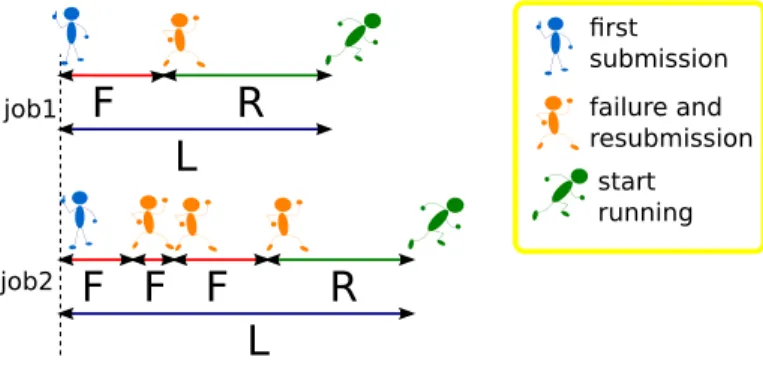
first submission failure and resubmission start running job1 job2Figure 1. Two examples of job submission with resubmissions in case of failures.
any notification). We denote as φ the fraction of jobs encountering a system fault and ρ the fraction of outliers.
B. Model of the grid jobs latency
Let R denote the proper latency of a successful job and F denote the failure time of a faulty job. Assuming that faulty jobs are resubmitted without delay, let L denote the job latency taking into account the necessary resubmissions (see figure 1). L depends on the distribution of the jobs failure time. The probability, for a job to succeed is (1 − ρ− φ). In practice, the values of ρ, φ, and the distributions of R and F are numerically estimated from grid monitoring traces while L is computed as shown below.
A job encounters a latency L < t, t being fixed, if it is not an outlier and either:
• the job does not fail (probability (1 − ρ − φ)) and its
latency R < t (probability P(R < t) = FR(t)); or • the job fails at t0< t (probability φfF(t0)) and the job
resubmitted encounters a latency L <(t − t0)
The cumulative distribution of L is thus defined recursively by:
FL(t) = (1 − ρ − φ)FR(t) + φ
Z t 0
fF(t0).FL(t − t0)dt0
As shown in a previous work [8], the cdf FL can be
numerically estimated by discretizing this equation (intro-ducing the second as the discretization step for the variable t) and observing that no successful job has a null latency (FR(0) = 0)4. This results in the following recursive
expression of FL: FL(0) = 0 FL(1) = 1 − ρ − φ 1 − φfF(0) FR(1) FL(t > 1) = 1 1 − φfF(0) h (1 − ρ − φ)FR(t) +φ t−1 X u=1 fF(t − u)FL(u) # (1)
4For a discussion on the validity of these hypotheses, refer to [8]
Under the hypothesis that failed jobs reporting requires at least one second (and therefore fF(0) = 0), this equation
simplifies: FL(0) = 0 FL(1) = (1 − ρ − φ)FR(1) FL(t > 1) = (1 − ρ − φ)FR(t) +φ t−1 X u=1 fF(t − u)FL(u) (2)
This hypothesis is valid in the sense that it has negligible impact on the jobs expected latency optimization procedure as will be shown later.
The probabilistic law L approximated through the discrete equation 2 can be exploited to numerically estimate the expected latency of jobs submitted to the grid infrastructure. This expectation depends on L and the resubmission strategy adopted as described in the following sub-sections. To be of practical interest, the derived expectation model needs to remain mathematically and computationally tractable.
C. Resubmission strategy and time-out estimation
Various client-side re-submission and multi-submission strategies have been considered in the literature to improve grid performance [7], [18]. In this paper we focus on the simplest and most common simple resubmission strategy, where a job is canceled and resubmitted if its latency is higher than a time-out value t∞. Poor estimations of the
time-out values can have strong performance impact: a lower time-out value will cause potentially successful jobs to be cancelled too early, while a higher time-out value will cause penalizing delays for non-successful jobs. However, the value of t∞can be determined through an optimization
procedure [1]. Let J denote the total latency experienced by a job, including as many resubmissions as needed after the time-out threshold t∞ has been reached.
A simplified model of the expected latency taking into ac-count resubmissions as a function of the time-out (EJ(t∞))
is proposed in [1]. However, this model excludes faults (faulty jobs were excluded from the statistics collection). To include faults in the resubmission process, we describe below two alternatives to this model (see figure 2):
J0 Jobs whom proper latency R is greater than the time-out
value t∞ are canceled and resubmitted. The resulting
total latency is denoted J0.
J1 Jobs for which the latency L, including resubmissions
due to faults, is greater than the time-out value t∞ are
canceled and resubmitted. The resulting total latency is denoted J1.
Strategy J1is an approximation of strategy J0when faults
occur: it does not take into account the time spent before fault notification in the resubmission delay. The time-out threshold will therefore be reduced by this period of time. However, the model of J1 is simpler and computationally
F
F
R
F
R
R >
L >
F
R
first submission failure and resubmission start running time-out, cancel and resubmissionFigure 2. Two ways of taking faults into account in the resubmission strategy J0(with time-out adapted dynamically in case of failures) and J1
(with fixed time-out, independently of failures).
more efficient. In [8], only strategy J1 was introduced. In
this paper, we also describe J0 and show how it can be
approximated by J1.
D. StrategyJ0
Strategy J0cancels and restarts a job only when its proper
latency is greater than the time-out value t∞. Since no job
has a null latency R, we have: fJ0(0) = 0
Before the time-out value t∞, no job has been canceled.
There are two possibilities for a job to have a total latency of t with0 < t < t∞:
• no failure and latency equal to t:(1 − ρ − φ)fR(t) • at least one failure at t0: φfF(t0)fJ0(t − t0)
leading to: fJ0(t) = (1 − ρ − φ)fR(t) + φ t−1 X t0=1 fF(t0)fJ0(t − t0)
After the time-out value t∞, the job has already at least
failed once or time-outed once. A time-out occurs in case of:
• outlier, with probability: ρ
• latency to failure greater than t∞, with probability:
φ(1 − FF(t∞))
• latency R greater than t∞, with probability: (1 − ρ −
φ)(1 − FR(t∞)) leading to: fJ0(t) = (ρ + (1 − ρ − φ)(1 − FR(t∞)) +φ(1 − FF(t∞)))fJ0(t − t∞) +φ t∞ X t0=1 fF(t0)fJ0(t − t0) 0 0.2 0.4 0.6 0.8 1 1.2 0 2000 4000 6000 8000 10000
cumulative density function of global latency F
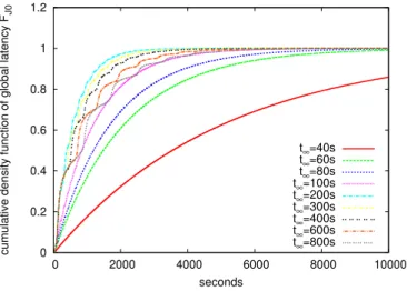
J0 seconds t∞=40s t ∞=60s t ∞=80s t∞=100s t ∞=200s t∞=300s t∞=400s t ∞=600s t∞=800s
Figure 3. Strategy J0. Cumulative density functions of global latency
including resubmission for different time-out values (t∞).
The complete expression of fJ0 is given by equation 3:
fJ0(0) = 0 fJ0(0 < t < t∞) = (1 − ρ − φ)fR(t) +φ t−1 X t0=1 fF(t0)fJ0(t − t0) fJ0(t ≥ t∞) = (ρ + (1 − ρ − φ)(1 − FR(t∞)) +φ(1 − FF(t∞)))fJ0(t − t∞) +φ t∞ X t0=1 fF(t0)fJ0(t − t0) (3) Figure 3 shows the profiles of the cdf total latency including resubmissions with strategy J0 corresponding to
different time-out values. The curve corresponding to t∞=
200 seconds is the closest to the optimal found among this sample: it displays the fastest convergence towards 1.
From the expression of fJ0 in equation 3, the latency
expectation computation is straight forward using its math-ematical definition:
EJ0(t∞) =
Z ∞ 0
tfJ0(t)dt (4)
A typical profile of the expectation of the total latency, as observed on a production grid, including all resubmissions and computed from equation 4, is plotted in figure 4. In this case, the curve reaches a minimum value EJ0 = 583s for an
optimal time-out value t∞ = 191s. An underestimation of
t∞ would cause early jobs cancellation, thus increasing the
number of resubmission and the total latency J0. Conversely,
an overestimation of t∞ would penalize the non-successful
jobs by late resubmission. This result is coherent with the observation from figure 3 where the best curve profile is obtained with t∞=200s.
E. Strategy J1
In strategy J1, in case of failure the job time-out is
not increased by the delay expired before failure reporting, thus under-estimating the time-out of the resubmitted job. Under this simplification hypothesis, the distribution of job latency including resubmissions fL can be used to derive
the distribution fJ in case of failure as observed in [8].
The latency J1 is therefore defined as a function of L and
t∞: a job for which L is greater than t∞ is cancelled
and resubmitted, thus increasing J1 by the time-out delay.
Observing that FL(t) corresponds to the probability for a
job to succeed with a latency lower than t, the probability for a job to time-out is q = P (L > t∞) = 1 − FL(t∞).
Denoting n the number of times the job timed-out (n is the integer such that t∈ [nt∞,(n + 1)t∞]):
FJ1(t) = P (L < nt∞)
+P (nt∞< L < t | t ≤ (n + 1)t∞)
= 1 − qn
+ qn
FL(t − nt∞)
(See [1] for details). Consequently, fJ1(t) = q
n
fL(t − nt∞)
and the expectation of J1 is EJ1(t∞) =
R∞ 0 ufJ1(u)du: EJ1(t∞) = 1 FL(t∞) Z t∞ 0 (1 − FL(u))du (5)
Minimizing this expression of EJ1 yields the optimal
time-out value t∞=195s for a minimal value EJ1 = 586s.
The profile of EJ1 is plotted on figure 4.
Note that the model of latency J1 was derived from
equation 2, assuming that fF(0) = 0. To validate this
hy-pothesis, the result obtained by this model can be compared to the one obtained by a model derived from equation 1 [8]. The impact on the estimated execution time is lower than 0.005%, confirming the hypothesis.
It should be noted that besides its more complex mathe-matical representation, model J0is significantly more
com-pute intensive than model J1. If we denote by t∞M AX the
upper bound of the interval of search for optimal timeout and n the number of samples needed for the computation of 4, the complexity of the computation of EJ in case of
J0 is in nt2∞M AX while it reduces to t 2
∞M AX in case of J1.
Numerically, we took t∞M AX = 1000 and n = 100000.
IV. QUANTIFYING THE IMPACT OF FAULTS ON RESUBMISSION STRATEGIES
The results obtained by exploiting strategies J0and J1are
compared to assess the performance of the simplified model in place of the exact one. Different experimental settings are considered to validate the results over infrastructures exhibiting different properties and under variable workload conditions along time. The first experiment targets realistic conditions as observed on the EGEE production grid in-frastructure. The second experiment targets different infras-tructures by varying the model parameters (ratios of faults,
500 600 700 800 900 1000 0 100 200 300 400 500 600
expectation of total latency E
J
timeout value (s)
EJ1 EJ0
without fault with faults as outliers
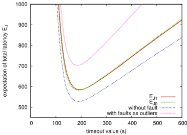
Figure 4. Expectation of total latency with respect to the time-out value t∞: cases of strategy J1, strategy J0, a simple model ignoring failures and
an approximation where failures are accounted as outliers.
outliers and distribution). The third and fourth experiments target workload variability as observed along time on the EGEE grid.
A. Impact on the EGEE production grid infrastructure
The data considered in this study are RTM/Grid Observa-tory traces of the EGEE grid activity during the period from September 2005 to June 2007. 33,419,946 job entries were collected, each of them representing a complete job run. Among these data, 64.8% corresponds to successful jobs, 19.1% to failures and the remaining 16.1% to outliers. The distribution of latency of successful jobs (R) and failure time of a faulty job (F ) are computed from these data.
Figure 4 displays several plots of the expectation of the total latency including resubmission. We observe that the results for strategies J0 and J1 are very close. In order
to compare the difference between J0 and J1 with other
hypotheses, EJ is also plotted for two other cases. The case
“without fault” where data corresponding to faulty jobs are neglected leads to an underestimation of EJ while the case
“with fault as outliers” where faulty jobs are considered as outliers leads to an overestimation of EJ.
This experiment shows that taking into account the latency for faults detection has a higher impact on the parameters estimation than the model used (J0 or J1). Moreover, for
J1, the best time-out value is t∞= 195s for an optimal EJ1
= 586s while, for J0, the best time-out value is t∞ = 191s
for an optimal EJ0 = 583s. If we would have chosen the
time-out value from J1 to be applied with strategy J0, we
would have obtained EJ0(195) = 583s (valued rounded to
integer value). The relative difference with the optimal value is negligible, in the order of 0.06%.
Looking at the distribution of faults detection latency fF
0 0.01 0.02 0.03 0.04 0.05 0.06 0.07 0.08 0.09 0.1 0 50 100 150 200
pdf of latency for faults detection f
F
seconds
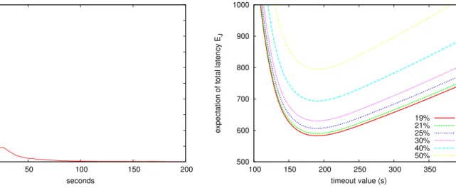
Figure 5. Probability density function of the latency for fault detection. We observe a maximum at 7 seconds.
582 584 586 588 590 592 594 180 185 190 195 200 205 210 215 220
expectation of total latency E
J
timeout value (s)
EJ1
EJ0
Figure 6. Zoom on the expectation of total latency for strategies J0and
J1.
with 50% of failures detected in no more than 10 seconds. On figure 6, we observe that variations of 10 seconds of time-out value around the optimal value does not increase the expectation of execution time by more than 2 seconds (0.3%). Consequently, J0and J1results are very close.
B. Impact on different workloads
J0 and J1 results are hardly differentiable under the
conditions observed on the EGEE production infrastructure during the period 2005-2007. Different workloads are sim-ulated by artificially varying the model parameters (failure distribution parameterization) in order to determine under which conditions the two strategies produce different results.
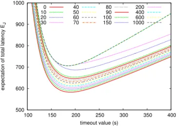
1) Varying the fault ratioφ: An increasing ratio of faults
φ is considered, ranging from the value measured on EGEE (19%) to 50% (see figure 7). They all conduct to an optimal
500 600 700 800 900 1000 100 150 200 250 300 350 400
expectation of total latency E
J timeout value (s) 19% 21% 25% 30% 40% 50%
Figure 7. Varying the ratio of faults φ in case of J0. The optimal time-out
value does not vary while the expectations of total latency are increasing. φ t∞0 EJ0(t∞0) t∞1 EJ0(t∞1) ∆% 19% 191 583 195 583 0.06 21% 191 590 195 590 0.08 25% 191 606 196 607 0.08 30% 191 630 198 631 0.14 40% 191 694 202 696 0.32 50% 191 795 207 780 0.61 Table I
COMPARISON OF STRATEGIESJ0ANDJ1WHEN VARYING THE RATIO OF FAULTSφ.
time-out value t∞0 = 191s in the case of J0. For each φ
value, we have computed the optimal time-out in the case of J1, t∞1, and compared the optimal value EJ0 with the
one obtained at t∞1. Results are reported in table I. Even
with the largest value of φ, the relative difference does not exceed 0.6%.
2) Translating the pdf of failure detection latency: As
another step toward worse experimental conditions, the latency of the faults detection delay was increased up to 1000 seconds (see figure 8).
For each delay of fault detection, the optimal time-outs t∞0 and t∞1 were computed with strategies J0 and J1, and
the expectation EJ0was estimated using both values. Results
are reported in table II. The relative difference grows up to 1.3% for an increased delay by approximately 90 seconds. For higher delays, relative differences are decreasing until 200 seconds where they do not vary any more: all faulty jobs encounter a time-out.
For delay increases smaller than 50 seconds, the relative difference is less than 0.6%.
From these artificial varying conditions on faults, we can conclude that, even with variations of faults ratio up to 50% and increase of pdf of latency for faults detection up to 50 seconds, numerically, results given by strategies J0 and J1
500 600 700 800 900 1000 100 150 200 250 300 350 400
expectation of total latency E
J timeout value (s) 0 10 20 30 40 50 60 70 80 90 100 150 200 400 600 1000
Figure 8. Translating pdf of failure detection latency: impact on EJ0.
Both optimal time-out value and expectation of total latency are varying. For translation higher than 200 seconds, results are similar since the optimal time-out is lower than 200 seconds.
t t∞1 t∞0 EJ0(t∞0) EJ0(t∞1) ∆% 0s 195s 191s 583.3s 583s 0.06 10s 198s 191s 591s 590s 0.1% 20s 202s 192s 599s 597s 0.3% 30s 206s 193s 607s 605s 0.4% 40s 208s 194s 614s 612s 0.5% 50s 211s 194s 622s 619s 0.6% 60s 214s 196s 630s 626s 0.7% 70s 219s 196s 639s 633s 1.0% 80s 223s 196s 648s 640s 1.2% 90s 225s 198s 655s 647s 1.3% 100s 218s 198s 690s 687s 0.5% 150s 187s 200s 690s 687s 0.4% 200s 185s 185s 707s 707s 0% >200s 185s 185s 707s 707s 0% Table II
COMPARISON OF STRATEGIESJ0ANDJ1WITH INCREASED FAILURE DETECTION LATENCY.
are very close.
C. Test on 2010 data
Recent data on the EGEE production infrastructure avail-able from the Grid Observatory (period from 2010-03-29 to 2010-04-04) was tested. After curation, 394315 data entries are suitable for computations. A classification of all entries, similar to [8] but adapted to new fault conditions reported (due to evolution of the middleware), was performed.
Compared to the data used in this paper, a lot of failures are reported very quickly, thus changing the profile of EJ
(see figure 9). However, EJstill exhibits a global minimum.
With a ratio of failure of φ = 25.8 % and a ratio of outliers of ρ = 9.4 %, the optimal time-out value t∞ is of 349
seconds for both J0 and J1: there is no added benefit to
consider strategy J0 instead of J1.
500 600 700 800 900 1000 0 200 400 600 800 1000
expectation of total latency E
J
timeout value (s)
EJ0 EJ1
Figure 9. 2010 data. Expectation of execution time including resubmis-sions for strategies J0 and J1: results are very similar even if the profile
differs from the one obtained with older data (see for example figure 4).
D. Test on 2009 data
Further tests were conducted using Grid Observatory / RTM data available earlier in 2009/2010: weeks 28 to 37 in 2009, week 14 in 2010. The results are identical for all weeks except the week 31 in 2009 where there is a relative difference of 0.02% between the expectation of total latency from the optimal values computed for strategies J0
and J1. The profiles of EJ are similar to the one presented
in figure 9.
V. CONCLUSION
Production grids usage is hampered by high failures rate and highly variable latencies observed in large scale complex systems. Efficient grid jobs resubmission therefore becomes a key feature of any grid experiment production environment. However, the scale of contemporary grids and their non stationary workloads makes optimal resubmission parameterization difficult.
In this paper, two probabilistic models of the simple grid jobs resubmission strategy were introduced. In case of failures, strategy J0 is properly taking into account the
time spent before failure notification in the estimation of the time-out threshold beyond which jobs are canceled and resubmitted. Strategy J1 is an approximation neglecting this
notification time.
Experiments with J0 and J1 using the same sets of data
show very close results in terms of expected latency time under variable workload conditions. This result has been validated both on real EGEE trace data at different times and on infrastructures with different faults distributions. The model can easily be adapted to other production environ-ments by measuring few infrastructure-specific parameters (i.e. ρ,φ,R,F ).
Strategy J0 is computationally more complex than J1,
that can be used as a valid approximation in practical im-plementations. This result can be extended and under similar conditions, we could benefit from this simplified model to address more elaborated client-side resubmission strategies such as multiple submission [7] and delayed resubmission with overlap of multiple instances of submitted jobs [18]. that are exploited by production grid users today.
ACKNOWLEDGMENT
The data sets used in this work have been provided by the Grid Observatory and the Imperial College London RTM. The Grid Observatory is part of the EGEE-III EU project, contract number INFSO-RI-222667.
This work is also partly funded by the French National Agency for Research, NeuroLOG project, under contract number ANR-06-TLOG-024.
REFERENCES
[1] T. Glatard, J. Montagnat, and X. Pennec, “Optimizing jobs timeouts on clusters and production grids,” in International Symposium on Cluster Computing and the
Grid(CCGrid’07). IEEE, May 2007, pp. 100–107. [Online].
Available: http://rainbow.polytech.unice.fr/publis/glatard-montagnat-etal:2007a.pdf
[2] E. Medernach, “Workload Analysis of a Cluster in a Grid Environment,” in Job Scheduling Strategies for
Parallel Processing(JSSPP), Jun. 2005, pp. 36–61. [Online].
Available: http://www.cs.huji.ac.il/˜feit/parsched/jsspp05/p-05-2.pdf
[3] L. Ilijaˇsi´c and L. Saitta, “Statistical Characterization of a Computer Grid,” in International Symposium on
Method-ologies for Intelligent Systems(ISMIS), vol. LNAI 5722.
Springer Verlag, Sep. 2009, pp. 523–532.
[4] A. Iosup, H. Li, M. Jan, S. Anoep, C. Dumitrescu, L. Wolters, and D. Epema, “The Grid Workloads Archive,” Future
Gener-ation Computer Systems (FGCS), vol. 24, no. 7, pp. 672–686,
Jul. 2008.
[5] D. Colling, J. Martyniak, S. McGough, A. Kˇrenek, J. Sitera, M. Mulaˇc, and F. Dvoˇr´ak, “Real Time Monitor of Grid job executions,” in Computing in High Energy Physics / Journal
of Physics: Conference Series(CHEP 2009). IOP Publishing,
Mar. 2009. [Online]. Available: http://www.iop.org/EJ/conf [6] C. Germain, C. Loomis, J. T. Mo´scicki, and R. Texier,
“Scheduling for Responsive Grids,” Journal of Grid
Com-puting (JOGC), vol. 6, no. 1, pp. 15–27, Mar. 2008.
[7] H. Casanova, “On the Harmfulness of Redundant Batch Requests,” in 15th IEEE International Symposium on High
Performance Distributed Computing(HPDC’06), Jun. 2006,
pp. 255–266.
[8] D. Lingrand, J. Montagnat, J. Martyniak, and D. Colling, “Optimization of jobs submission on the EGEE production grid: modeling faults using workload,” Journal of Grid
Com-puting (JOGC) Special issue on EGEE, vol. 8, no. 2, pp.
305–321, Mar. 2010.
[9] X. Zhang, M. Sebag, and C. Germain, “Multi-scale Real-time Grid Monitoring with Job Stream Mining,” in 9th IEEE/ACM International Symposium on Cluster Computing and the
Grid(CCGrid), May 2009, pp. 420–427. [Online]. Available:
http://www.lri.fr/˜xlzhang/papers/ccgrid09 zhang.pdf [10] H. Eichenhardt, R. M¨uller-Pfefferkorn, R. Neumann, and
T. William, “User- and job-centric monitoring: Analysing and presenting large amounts of monitoring data,” in 9th
International Conference on Grid Computing(IEEE Grid).
IEEE, Sep. 2008, pp. 225–232.
[11] D. Cieslak, N. Chawla, and D. Thain, “Troubleshooting thousands of jobs on production grids using data mining techniques,” in 9th International Conference on Grid
Computing(IEEE Grid). IEEE, Sep. 2008, pp. 217–224.
[On-line]. Available: http://www.nd.edu/˜ccl/research/pubs/debug-grid08.pdf
[12] G. Maier, D. C. Vanderster, and D. Kranzlmueller, “Finding associations in Grid monitoring data,” in 10th International Conference on Grid Computing(IEEE
Grid). IEEE, Oct. 2009, pp. 89–96. [Online]. Available:
http://maierg.web.cern.ch/maierg/documents/grid09 paper.pdf [13] C. Dabrowski, “Reliability in grid computing systems,” Concurrency and Computation: Practice & Experience
(CCPE) Special issue on Open Grid Forum,
vol. 21, no. 8, pp. 927–959, Jun. 2009. [Online]. Available: http://www.nist.gov/itl/antd/upload/Dabrowski-GridReliabilityEarlyView.pdf
[14] E. Frachtenberg and U. Schwiegelshohn, “New Challenges of Parallel Job Scheduling,” in 13th
Job Scheduling Strategies for Parallel
Process-ing(JSSPP), vol. LNCS 4942. Springer, Apr. 2008,
pp. 1–23. [Online]. Available: http://www.it.irf.uni-dortmund.de/IT/Publikationen/pdf/FS08.pdf
[15] E. Huedo, R. S. Montero, and I. M. Llorente, “Evaluating the reliability of computational grids from the end user’s point of view,” Journal of Systems Architecture, vol. 52, no. 12, pp. 727–736, Dec. 2006.
[16] O. Thebe, D. P. Bunde, and V. J. Leung, “Scheduling Restartable Jobs with Short Test Runs,” in 14th Workshop on Job Scheduling Strategies for Parallel Processing(JSSPP’09),
workshop: IPDPS, vol. LNCS 5798. Springer, May 2009,
pp. 116–137.
[17] T. Glatard and S. Camarasu-Pop, “Modelling pilot-job appli-cations on production grids,” in 7th international workshop on Algorithms, Models and Tools for Parallel Computing on
Heterogeneous Platforms(Heteropar’09), Aug. 2009.
[18] D. Lingrand, J. Montagnat, and T. Glatard, “Modeling user submission strategies on production grids,” in International Symposium on High Performance Distributed
Computing(HPDC’09), Jun. 2009, pp. 121–130. [Online].
Available: http://rainbow.polytech.unice.fr/publis/lingrand-montagnat-etal:2009.pdf