HAL Id: hal-01110642
https://hal.archives-ouvertes.fr/hal-01110642v2
Submitted on 4 Jun 2017
HAL is a multi-disciplinary open access
archive for the deposit and dissemination of sci-entific research documents, whether they are pub-lished or not. The documents may come from teaching and research institutions in France or abroad, or from public or private research centers.
L’archive ouverte pluridisciplinaire HAL, est destinée au dépôt et à la diffusion de documents scientifiques de niveau recherche, publiés ou non, émanant des établissements d’enseignement et de recherche français ou étrangers, des laboratoires publics ou privés.
Deleveraging crises and deep recessions: a behavioural
approach
Pascal Seppecher, Isabelle Salle
To cite this version:
Pascal Seppecher, Isabelle Salle. Deleveraging crises and deep recessions: a behavioural approach. 3rd International Symposium in Computational Economics and Finance (ISCEF), Apr 2014, Paris, France. �hal-01110642v2�
This is an Accepted Manuscript of an article published by Taylor & Fran-cis in Applied Economics on 26/04/2015, available online:
http://www.tandfonline.com/doi/full/10.1080/00036846.2015.1021456.
Deleveraging crises and deep recessions: a behavioural
approach
∗Pascal Seppecher† & Isabelle Salle‡
October 30, 2014
Abstract: Macroeconomic dynamics are characterized by alternating patterns of periods of relative stability and large swings. Standard micro-founded macro-economic models account for these patterns through exogenous and persistent shocks. In this paper, we develop a fully decentralized and micro-founded macro-economic agent-based model, augmented with an opinion model, which produces endogenous waves of pessimism and optimism that feed back into firms’ leverage and households’ precautionary saving behaviour. A major emergent property of our model is precisely the complex successions of stable and unstable macro-economic regimes. The model is further able to account for a wide spectrum of macro- and micro empirical regularities. Within this framework, we analyse a series of macro-economic phenomena of key relevance in the current macro-economic debate, especially the occurrence of deleveraging crises and Fisherian debt-deflation recessions. Our analysis suggests that the relative dynamics of prices and wages and the resulting income distribution along a deflation-ary path are critical determinants of the severity of the recession, and the chances of recovery. Keywords: Agent-based modelling, Deleveraging crisis, Opinion dynamics, Prices-Wages Dynamics.
JEL-classification: E20; E12; E32; C63
∗We are grateful to the participants of the internal seminar at the Catholic University in Milan, on January
15, 2014, in particular to Prof. D. Delli Gatti and Prof. C. Hommes, for helpful discussions and feedbacks on an earlier version of this paper. We also thank participants and organizers of the 3rd ISCEF conference, on April 10-12, 2014 in Paris, as well as Dr. M. Zumpe and three anonymous referees and an editor for interesting comments that helped us to improve this work. Isabelle Salle acknowledges financial support from the EU FP7 RAstaNEWS project, grant agreement No. 320278.
†Centre d’Economie de Paris Nord (CEPN) - UMR CNRS 7234 - University of Paris Nord & Groupe de
Recherche en Droit, Economie, Gestion (GREDEG), UMR CNRS 7321 - University of Nice Sophia Antipolis - France; Corresponding author: [email protected]
‡CeNDEF, Amsterdam School of Economics, UvA, & Tinbergen Institute, the Netherlands, & University
1 Introduction
Developed economies are characterized by alternating patterns of periods of relative stability and large swings in economic activity. The Great Moderation period, and the recession following the 2007-8 financial crisis are a good example of these patterns. Which mechanisms can drive and amplify such economic downturns, and which conditions may allow for a recovery are the central issues at stake in this paper.
Standard micro-founded macro-economic models – such as DSGE models – account for fluctuations through (large) exogenous and persistent shocks added to the aggregate equations of the model. The growing literature on behavioural (macro)-economics takes a different view.
Its heterogeneous agent strand (see the seminal contribution of Brock & Hommes (1997))
has given interesting insights into the endogenous emergence of booms and busts in a New
Keynesian model (see more particularly De Grauwe(2011, 2012)). This modelling strategy
relies on general equilibrium frameworks, that are derived from the assumption of optimizing representation agents.
Its (macro) agent-based strand has also produced models that are able to create
endoge-nous business cycles.1 In a nutshell, ABMs are the representation of a decentralized market
economy as a complex system: "Large numbers of micro agents engage repeatedly in local interactions, giving rise to macro regularities such as employment and growth rates, income distributions, [...] These macro regularities in turn feed back into the determination of local interactions. The result is an intricate system of interdependent feedback loops connecting micro behaviour, interaction patterns, and global regularities", (Tesfatsion (2006, p.191)). These models are analysed though numerical simulations. ABMs provide micro-foundations to macroeconomic models by relying on two main ingredients, namely heterogeneity and pro-cedural/bounded rationality. In these models, a collection of heterogeneous agents locally in-teracts without seeing the whole picture of the economy. Consequently, agents cannot identify optimal plans given the whole relevant information, and are instead endowed with
procedu-ral rationality (Simon(1962)): agents aim at simplifying their decision making by adopting
simple adjustment rules – or heuristics.
This paper presents an analysis within such an ABM of the endogenous emergence of deleveraging crises, the following recession episodes, and the conditions of the recovery. We
elaborate on the macroeconomic ABM of Seppecher (2012) – the Jamel model2 – because
it exhibits several interesting features, both compared to most DSGE models and existing 1The interested reader can consult Prof. Leigh Tesfatsion’s website athttp://econ2.econ.iastate.edu/
tesfatsi/amulmark.htm, which offers a rich library of the models which have been developed in this literature.
Major contributions in this field include (without exhaustiveness) the "K+S" model ofDosi et al.(2010,2013), the Eurace@Unibi model (Dawid et al.(2014)), the models fromLengnick(2013) andRiccetti et al.(2012), the "Mark 0 to 2" models ofDelli Gatti, Desiderio, Gaffeo, Cirillo & Gallegati(2010). We refer mostly to these contributions when referring to the state-of-the-art of macro ABMs.
ABMs. The Jamel model is a fully decentralized economy and is stock-flow consistent. De-centralization ensures that prices and wages stem from the local interactions in the labour
and the goods markets, and that the resulting income distribution is endogenous.3 Stock-flow
consistency ensures that there is no leakage in the model, and all agents’ balance sheets are linked together (Caverzasi & Godin(2013)). These characteristics are of particular relevance for the analysis of business cycles and crises, especially debt and leverage of firms, saving and consumption decisions of households, income distribution and wage/price dynamics.
Further-more, the Jamel model copes with the so-called "wilderness of bounded rationality"4 in a
twofold way, both within the design of its behavioural rules and at the stage of the numeri-cal simulations. First, when constructing the model, we ensure the consistency of the micro behavioural rules by applying a common pattern for most agents’ decisions in the model. Agents successively adjust their behaviour by observing unbalances between their actual and their targeted levels of their variables. These targeted levels can be understood as
satisfyc-ing (Simon(1955)). This literature has also been extended with empirical and experimental
evidence (seeHommes (2011) for a survey). Second, when running the model, we follow the
state-of-the-art practice in macro ABM, and perform an extensive exercise of empirical vali-dation. This exercise shows that the micro behavioural ingredients of the model allow for the emergence of both micro and macro patterns, that are in line with stylized facts highlighted by
the empirical literature. The main emergent feature of the Jamel model inSeppecher(2012)
is a long-run stabilization of the macroeconomic variables with small fluctuations around a "steady state". Large fluctuations are only obtained as a result of exogenous shocks on the parameter values.
In this paper, we extend the Jamel model by introducing an opinion dynamics model, which allows the state of the economy to feed back into the agents’ behaviour. The agents adjust their financial behaviour as a result of their market sentiment, which we summarize in two possible states: either optimistic or pessimistic. This market sentiment is partly driven by the agents’ own individual situation, and a herding component, which models contagion of optimism and pessimism between the agents. In economics, contagion models have been mostly applied to herding behaviour in finance as a endogenous source of asset price
fluctuations.5 Our opinion model also relates to the model of recruitment process among ants
developed in Kirman (1993), in which ants have two states, and can convert each other or
self-convert with some exogenous probabilities. Interestingly, the "ant model" gives rise to the 3ABMs often focus on disaggregating one sector (usually firms and/or banks), leaving one side of the
mar-kets (usually households) to be determined as an aggregate component, and, hence, leaving the determination of at least some variables as an aggregate process. Notable exceptions include Riccetti et al. (2012) and
Lengnick(2013).
4The expression is due to C. Sims, and refers to the fact that modelling non-optimizing agents can be done
in a multitude of ways, by contrast to optimization.
5A (non-exhaustive) list of contributions includes Lux (1995,1998), Sornette (2003), Akerlof & Shiller
(2009),Bouchaud(2013). The closest to our opinion model isTedeschi et al.(2012), where traders rely either on their own opinion, or the one of their neighbours with an exogenous probability.
same pattern of endogenous and unpredictable switching between these two states as the waves of pessimism and optimism that we observe in our model. We call these endogenous waves "animal spirits", as a reference to Keynes (1936) and, more recently, to De Grauwe (2011,
2012). De Grauwe uses a heuristic switching model6 in which agents switch from pessimistic
to optimistic expectations, and shows how this creates endogenous business cycles in a New Keynesian model. Such contagion models are able to account for complicated dynamic as a result of simple individual behaviour. Also related to our modelling strategy is the model
of epidemiology in Carroll et al. (2003), which explains the transmission of news among a
population of agents.
In our framework, we observe two main phenomena. First, the emergent macroeconomic dynamics display alternating patterns of periods of relative stability and large swings, a fea-ture which was completely absent from the previous versions of Jamel. Second, the economic downturns that we observe along the business cycles resemble the deleveraging crises as
dis-cussed in Eggertsson & Krugman (2012). Importantly, we stress that these emergences are
endogenous. No exogenous process is present in the model, which could trigger the observed economic downturns. "Animal spirits" play the critical role in those emergences. Animal spir-its amplify the small fluctuations that stem from the agents’ adjustment behaviour, and cre-ate cascade effects in the agents’ market sentiment, and in their resulting financial behaviour. Their financial behaviour in turn feeds back into the aggregate activity, and confirms the mass movements in market sentiment. As a result, animal spirits interconnect micro behaviour and aggregate dynamics in a positive feedback system. In our setting, an extended period of economic stability encourages relaxed views about what level of debt (firms’ leverage) is ac-ceptable, and encourages households to decrease their precautionary savings, because most firms and households are optimistic. However, at some point, the increased level of debt and the decreased level of savings put some households and firms under financial stress, turning them into pessimistic agents. As a result, those agents start a sudden deleveraging and sav-ing process. This translates into a decrease in consumption expenses, debt and dividends. This in turn leads to a slow down in aggregate activity and a debt-driven slump, so that the pessimistic views turn out to be self-validating, and animal spirits propagate pessimism among the agents. This wave of pessimism drives the economy towards a deep recession. This
phenomenon is known as the Fisherian debt-deflation dynamics (Fisher(1933)).
Within our framework, we then address the question of the drivers of the recovery along such a deflationary path. Our model strongly suggests that the end of the recession critically depends on the way the debt-deflation spiral affects income distribution and the relative dynamics of prices and nominal wages. If prices fall quicker than nominal wages do, real wages end up increasing, so that a demand-driven recovery is made possible. This recovery
occurs well before the deleveraging process of the firms is completed, or the households’ precautionary savings objective is reached. On the contrary, if nominal wages fall faster than prices do, real wages decrease along a debt-deflation path, and our model suggests that a demand-driven recovery is no longer possible. Admittedly, the relative rise in profits repairs the firms’ balance sheets, and allows them to get closer to their deleveraging objective, which may create the conditions of a recovery. However, in that case, the recession appears much deeper and longer-lasting than in the case where a demand-driven recovery is made possible. This type of emergent dynamics is of particular relevance regarding the current economic debates in the wake of the 2007-8 financial crisis and the Great Recession which has followed, and we provide some elements of policy discussion.
The rest of the paper is organized as follows: Section2introduces our ABM – the Jamel
model, numerical simulations are reported in Section3and Section4concludes.
2 The Jamel model
The economy is populated by n heterogeneous households, indexed by i = 1, ..., n, m hetero-geneous firms, indexed by j, j = 1, ..., m, and one bank. The firms produce an homohetero-geneous consumption goods by using capital (assumed to be fixed) and labour. Labour is supplied by the households, who also consume the goods. The bank provides loans to the firms to finance their production (wage bill), and hosts households’ savings (as cash deposits). The firms and the bank are assumed to be owned by households, who then receive dividends. Those owners are randomly drawn among households at the beginning of each simulation, and remain the same for the whole simulation.
2.1 Timing of the events
As ABMs are sequential models, we have to make the timing of events explicit. One period t corresponds to a month, as wages are usually monthly payments. In each period, the following steps prevail:
1. Households who own the firms and the bank receive dividends.
2. The firms set up their production plan (labour to hire, quantity to produce, price to set, wage to offer, and financial needs), and borrow money from the bank accordingly, in order to finance their wage bill.
3. The labour market opens, and matches the firms’ labour demands with the households’ labour supplies. This process yields the households’ labour incomes and the firms’ production plan is implemented.
5. The goods market opens, and matches the households’ demand with the firms’ supply. This process updates the firms’ inventories and their profits.
6. The firms pay back part of their loans and the interests to the bank.
7. The firms and the bank decide the amount of the dividends to pay to their owners. 8. This process starts all over again for a given length of T periods.
We now fully describe the behaviour of each category of agents.
2.2 The households
2.2.1 Labour supply and wage
Each household i is endowed with a one-unit labour supply, denoted by hi,t = 1, ∀i, t. The
households’ decision variable in the labour market is the reservation wage, denoted by ˆwi,t.
If an household i is employed, his reservation wage equals his wage, i.e. ˆwi,t = wi,t. If an
household i is unemployed, he does not receive any wage (i.e. wi,t= 0), and his reservation
wage is adjusted downward, depending on his unemployment duration du
i,t, i.e. the number of periods since his last job. This behavioural rule finds empirical support in micro studies, e.g.
Burdett & Vishwanath(1988). The reservation wage of an unemployed household i in period tevolves as:
ˆ
wi,t= ˆwi,t−1(1− δwi,t) (1)
where δw
i,t≥ 0 is the size of the downward adjustment, and is computed as:
δi,tw = βi,t· ηH if αi,t< du i,t dw 0 else. (2)
where αi,t, βi,t are U(0, 1), and ηH > 0 and dw≥ 1 are parameters. Accordingly, the proba-bility of decreasing the reservation wage ˆwi,t increases with the unemployment duration dui,t.
After dwperiods being unemployed, i.e. when du
i,t≥ dw, the first condition of Eq. (2) always holds, and the adjustment becomes systematic. In addition, the individual stochastic
com-ponents αj,t and βj,t result in heterogeneous adjustments, even between households with the
same unemployment duration.
2.2.2 Consumption plan and consumer sentiment
We make two assumptions regarding the consumption rule in the model. First, the households follow a general pattern of consumption smoothing in face of unanticipated income variations
by building precautionary savings (at a zero-interest rate). We follow here, inter alia, Allen
consumer sentiment, i.e. whether the household is pessimistic or optimistic about the state of the affairs in the economy. More pessimistic views about future economic developments refrain consumption, and incite households to build up more precautionary savings. This behaviour has been characterized as prudence in the related literature about savings and uncertainty that we follow there – e.g. Kimball (1990),Carroll et al.(1994) orHauenschild & Stahlecker
(2001). This behaviour also implicitly underlies the positive relationship between current and
expected consumptions in the usual Euler relation.
In line with these two assumptions, the households follow a buffer-stock rule, and cannot
borrow. Each household computes his cash-on-hand target sT
i,tas a fraction κS,i,tof his average monthly income over the last twelve months/periods, denoted by ˜yi,t, i.e. sTi,t = κS,i,t· ˜yi,t.
Each household then computes his targeted consumption expenditures cT
i,tas: cTi,t=
(1− κS,i,t)˜yi,t if si,t≤ sTi,t ˜
yi,t+ µH(si,t− sTi,t) else.
(3)
where µH ≥ 0 is a parameter. According to Eq. (3), if his cash-on-hand at time t, denoted
by si,t, is lower than his targeted level sTi,t, household i intends to spend only a fraction κS,i,t of his average income, and saves the rest. If his effective cash-on-hand is higher than his
targeted level, household i intends to spend all his income and a fraction µH of his excess
cash-on-hand in the goods market.
The targeted fraction of cash-on-hand κS,i,t of each household i can take two values
de-pending on his consumer sentiment. If he is optimistic, household i targets a low fraction of cash-on-hand to be held as precautionary savings, i.e. κS,i,t= κS. If pessimistic, he targets a high fraction of cash-on-hand, i.e. κS,i,t= ¯κS> κS. Each household i switches between these two targets depending on his consumer sentiment.
2.2.3 Opinion dynamics
Each household i’s consumer sentiment, i.e. whether he is pessimistic or optimistic, evolves through a model of opinion dynamics. The opinion dynamics model relies on both the individ-ual state of each household, and an "animal spirit" component, through which the household is influenced by some other households’ opinion. We take the employed or unemployed status of each household has a evaluation criterion of his own individual situation. Several empirical studies document the relationship between the level of unemployment and pessimism among
private agents (e.g. Artus(2013)), and between precautionary savings and the risk of
unem-ployment (Carroll et al. (2003)). The design of this opinion dynamics model is borrowed to
the contagion models that have been applied to herding behaviour in financial markets – see the literature review that we provide in the introduction.
In each period t, each household i observes the consumer sentiment of h < n other
house-holds7, and updates his consumer sentiment, and his corresponding targeted fraction of
cash-on-hand as follows:
• With a probability 1 − p, household i relies on his own individual situation: if he is unemployed, he is pessimistic and sets κS,i,t= ¯κS, and if he is employed, he is optimistic, and sets κS,i,t= κS.
• With a probability p, household i relies on the majority opinion among the h other households: if most are pessimistic, he is pessimistic, and sets κS,i,t = ¯κS, and if most are optimistic, he is optimistic and sets κS,i,t= κS.
Accordingly, we define the probability p as the strength of "animal spirits" in the model. 2.2.4 Budget constraint
Finally, in each period t, any household i’ budget constraint is given by:
ci,t≤ wi,t+ di,t+ si,t−1≡ si,t (4)
where di,t is the dividend that household i may receive if he owns the bank or a firm (see
below), wi,tis his labour income, st−1,ihis cash-on-hand transferred from the last period, and ci,this (effective) consumption expenditures. We then have ci,t= min(cTi,t, si,t).
2.3 The firms
2.3.1 Production function
Each firm j is endowed with a fixed amount of Kj = K units of capital, ∀j (each unit
can be understood as a machine). Each machine has the same productivity, equal to prk.
Hence, there is no capital accumulation dynamics through investment in the model. The firms combine labour with machines in order to produce, and production factors are assumed
to be complementary (e.g. Delli Gatti, Gallegati, Greenwald, Russo & Stiglitz(2010)). The
maximum labour force that a firm can hire is then given by the number of machines K, which
also defines the production capacity of each firm per period, namely K · prk. Production is a
time-consuming process, and spreads out over several successive periods (Keynes (1936)): in
each period t, each worker can only work on a single machine, and increment its production
process by one step. Each machine needs dm steps to complete the production process, so
that it takes at least dmperiods for a machine to deliver an output, and after completion, this
output is given by prk units of goods. When hiring workers, the machines whose production
7This process is similar to the tournament selection in genetic algorithm-based learning models, e.g.Vriend
process is the most advanced are prioritized. Each time a production process of a machine
of firm j comes to the end, the resulting output prk is added to firm j’s inventories level,
denoted by inj,t.
2.3.2 Production plan decisions
In each period t, each firm j decides about her production plan by successive adjustments.
Labour demand Inventories have a twofold role (Cyert & March(1963)). First, we assume
that the each firm tries to maintain an inventory level inj,tas a buffer to cope with unexpected
variations of her environment. The targeted level of inventories corresponds to din periods of
production at full capacity, i.e. equals inT = d
in· K · prk (and is the same across all firms). Second, the firms take variations in the level of their inventories as a proxy for variations of
their demand. If the effective level of inventories inj,t is lower that the targeted one (first
condition of Eq. (6) below), this may be a sign of excess demand, and firms are likely to
increase production and, hence, their labour demand. Conversely, if effective inventories are higher than the targeted level (second condition of Eq. (6) below), firms are likely to decrease production and to fire workers, the latest hired being fired first. Hence, in each period t, the
labour demand hd
j,tof each firm j evolves (within the lower bound 0 and the upper bound K)
as follows:
hdj,t= (1 + δhj,t)hj,t−1 (5)
where hj,t−1is the effective labour hired by firm j in period t−1 (after matching in the labour
market, see Subsection2.5), and δh
j,t is the size of the adjustment, computed as:
δhj,t= αj,t· νF if 0 ≤ αj,tβj,t< in T−in j,t inT −αj,t· νF if 0 ≤ αj,tβj,t< inj,t−in T inT 0 else. (6)
with αj,t, βj,t,→ U(0, 1) and νF > 0a constant. Eq. (6) translates both a principle of reaction
to stress and a principle of conservatism (Cyert & March (1963)). On the one hand, the
probability of firm j to adjust her labour demand increases when the observed unbalances in inventories increase (to see this, notice that the higher the inventory gap, the higher|inT−in
j,t|
inT ,
and the more likely the first or the second condition of Eq. (6) to hold). On the other hand,
we have αj,tβj,t ≤ 1, which makes the adjustment non-systematic even in case of a non-zero
inventory gap. Moreover, the higher αj,t, the higher the resulting adjustment, and the less
likely to be adopted, which implies a conservative reaction from the firms (to see this, notice that the higher αi,t, the more likely the first or the second condition of Eq. (6) to be violated,
and the more likely to have δh
αj,t and βj,t result in heterogeneous reactions, even between firms facing the same inventory gap.
Goods supply As firms use inventories to dampen market variations, they always keep a
fraction 1 − µF of their inventories inj,t as a buffer. We also assume that each firm has a
maximum market capacity, which we take to be equal to her inventory target inT. In each
period t, each firm j goods supply is therefore given by:
yj,t = min(µF.inj,t, inT) (7)
Price setting Similarly to the labour demand decision, prices may be increased in reaction
to a lower-than-targeted level of inventories, and vice-versa. We further assume that each firm faces so-called "menu costs", and can only adjust her price every dp periods. This allows to
control for price stickiness in the model, through aCalvo (1983)-like process. In case a firm
can adjust her price in a given period t, she increases her price if her inventories are lower than the targeted level and she was able to sell all her production during the last period. Conversely, a firm decreases her price if her inventories are higher than the target and she got unsold quantities after the matching process in the goods market. In case an adjustment takes place, its size is the same as δh
j,t given by Eq. (5), and the resulting price is given by:
pj,t= (1 + δhj,t)pj,t−1 (8)
Otherwise, the firm leaves her price unchanged.
Those behavioural rules imply rigidities in the adjustment of prices and quantities for two reasons. First, this is because stochastic components in Eq. (6) and (9) (see hereafter) imply that adjustments in face of changes in demand are not systematic. Second, this is because firms are not allowed to adjust their prices every period.
Wage offer Firms adjust their wage offer wj,t in a similar way as they adjust their labour
demand. Each firm computes her vacancy rate ρj,t ≡ K−hKi,t. We assume that she has a
targeted level of vacancies, exogenously fixed to ρT for all firms. A higher-than-targeted
vacancy rate (see the first condition of Eq. (9) below) is interpreted as a sign of an excess
labour supply over demand, and leads to a decrease in the offered wage, and vice-versa (see
the second condition of Eq. (9)). Formally, we have:
δj,tw = αj,t· νF if 0 ≤ αj,tβj,t < ρT − ρj,t −αj,t· νF if 0 ≤ αj,tβj,t < ρj,t− ρT 0 else. (9)
The resulting wage offer of firm j in period t is then:
wj,t= (1 + δwj,t)wj,t−1 (10)
The duration of the offered contract is set to dw> 1periods, and the wage remains fixed for
this whole period.
2.3.3 Financial decisions and business sentiment
The firms estimate their expected wage bill in case all the vacancies will be filled, i.e. wj,t·hdj,t.
In case the bill is higher than the available cash-on-hand of the firm (that we denote mj,t),
she borrows from the bank (see Sub-section 2.4 how the loans are granted). Formally, the
credit demand of firm j in any period t is max(wj,thj,t− mj,t, 0).
Each firm may distribute dividends dj,t. We assume that each firm j has a leverage target
(1− κF,j,t)≥ 0, where the leverage is the ratio between the liabilities (debt) of the firm and
her total assets denoted by Aj,t. Conversely, the corresponding targeted level of net wealth is
given by nwT
j,t = κF,j,tAj,t. Only if the actual net wealth nwj,t is higher than the targeted one will dividends be distributed. In that case, the firm distributes the excess net wealth within the limit of her available cash-on-hand:
dj,t = nwj,t− nwj,tT if 0 < nwj,t− nwTj,t≤ mj,t mj,t if nwj,t− nwj,tT > mj,t> 0 0 else. (11)
As for the households, the firms can be either pessimistic or optimistic regarding the state of the affairs in the economy. The targeted level of net wealth κF,j,tof each firm j can take two values depending on her business sentiment. Pessimistic firms have a high net wealth target or, put differently, a low leverage target (1 − ¯κF), and optimistic firms have a high leverage target (1−κF), where κF < ¯κF.8 Firms switch between optimism (and a high leverage target) and pessimism (and a low leverage target) according to exactly the same opinion dynamics model as for households. In particular, probability p and the size of the neighbourhood h
are the same (see Sub-section 2.2). The only difference is the evaluation criterion of each
firm’s own individual situation. We take the evolution of the anticipated demand, that we
compute as the average of past sales, for such a criterion (see Dosi et al.(2010, 2013) for a
similar assumption). Formally, with a probability 1 − p, a firm looks at her own situation, and is optimistic if the past level of her sales exceeds sF% of the total market capacity of the firm, and is pessimistic otherwise. With a probability p, the firm adopts the majority opinion 8See, e.g., Sharpe (1994), Hackbarth(2009),Geanakoplos (2010) or Eggertsson & Krugman (2012) for
among h other firms.
2.4 The bank
The main role of the bank is to provide loans to the firms to finance their wage bill. As this role is essentially passive, the banking sector is summarized by a single bank. At a first step, the bank is fully accommodative, and satisfies all the credit demands from the firms. Loans
are granted for a period of dl months, at a fixed interest rate r. However, when a firm is not
able to pay off a loan in due terms, the due period is extended to d0
l, the interest rate is set at
a higher level r0, and the debt is downgraded to doubtful debt, reflecting the increasing risk
of the firm’s loan. When a firm cannot pay off a doubtful debt, she goes bankrupt, and the bank absorbs the failing firm’s debt through its own resources (i.e. interest-payments from the firms). The bank then uses those resources in order to recapitalize up to its targeted level:
in the exact same way as the firms, this targeted level is a proportion κB of the total assets
of the bank, and excess is distributed as dividends to its owner in the exact same way as in
Eq. (11). Note that in the case of a bankruptcy, a new firm will be created tf periods later
(we reset all variables of the firm), in order to avoid a mechanical concentration in the goods market.
2.5 Markets and dynamics
The markets are decentralized and interactions are based on a tournament selection procedure (Riccetti et al.(2012)): each seeker only consults a subset of offers, and selects the one which fulfils the most his objectives. Aggregate variables simply consist of the sum of individual ones.
In the labour market, each firm posts hd
j,t offers at a given wage wj,t. Each unemployed
household consults g offers, and selects the one with the highest wage, provided that this wage is at least as high as his reservation wage ˆwi,t. Otherwise, he stays unemployed.
In the goods market, each firm posts offers with her given goods supply yj,t at the price
pj,t, and each household enters with his desired level of consumption expenditures cTi,t. Each household selects a subset of g firms, and chooses to buy to the cheapest one. This process is repeated until the total budget of all consumers or the total quantity of goods are exhausted.
We now turn to the numerical simulations of the model.9
3 Numerical simulations
We first define a baseline scenario following empirical validation criteria. We then analyse this baseline scenario, and contrast it with an alternative one to shed light on the origins of 9The model is implemented as a Java application, that is executable at http://p.seppecher.free.fr/
the crises, the ensuing dynamics and the conditions of the recovery.
3.1 Empirical validation: a baseline scenario
The model involves many parameters, whose values cannot necessary be set based on empirical
estimations. Following the latest methodology in macro ABM (Windrum et al. (2007)), we
perform an empirical validation exercise. We select parameter values so that the model is able to capture a reasonably wide set of stylized facts, both at the macro and at the micro levels,
and we define this calibration as the baseline scenario. Table 1 gives the corresponding
parameter values. The statistics reported below are averages and standard deviations across
30replications of the baseline scenario with different seeds of the random number generator.
The low values of standard deviations across those replications demonstrate that the aggregate behaviour of the model is quite stable, and qualitatively insensitive to stochastic elements, so that 30 replications appear enough to ensure robustness.
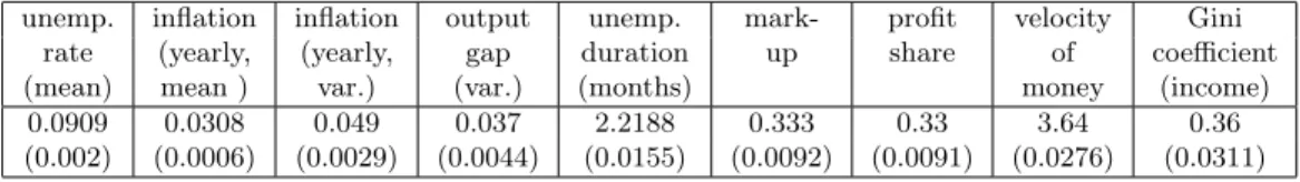
[Table 1 about here.] 3.1.1 Business cycles and macroeconomic regularities
Table2reports the average and standard deviations of the major macroeconomic variables in
the baseline scenario, namely the mean of unemployment rate, the inflation rate (both mean and variability), the variability of output gap, the unemployment duration, the mark-up of firms over costs, the profit share and the velocity of money. The resulting values are in line
with empirical observations.10
[Table 2 about here.]
Our model is also able to reproduce stylized facts on business cycles (see Stock &
Wat-son (1999)). In particular, consumption and output time series are strongly and positively
correlated, both display an alternate of smooth phases and strong fluctuations (Figure 4c
hereafter), with consumption being less volatile than output (see Table3).11
[Table 3 about here.]
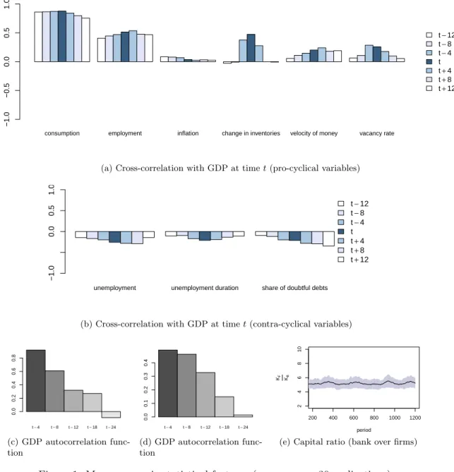
Furthermore, consumption, employment, changes in inventories (relative to GDP), infla-tion, the vacancy rate and the velocity of money appear pro-cyclical, while the unemployment rate, the unemployment duration and the share of doubtful debts are contra-cyclical (see
Fig-ure1aand Figure1b). Inflation is then demand-driven, in line with the absence of cost-push
10In developed countries, the profit share is close to one third of the income. We obtain about 10 weeks
for the average unemployment duration, which roughly matches the OECD data in the 2000’s. The average mark-up varies across sectors, but we obtain around 30%, which falls into the range of usual estimations.
11Following standard practices in macro time series analysis, all time series have been bandpass filtered, and
represent deviations from a long term average value, seeBaxter & King(1999). Plots correspond to one run of the model, and statistical significance of the results is systematically established using the 30 replications of this run.
shocks in the model. The share of doubtful debt and employment are lagging and consump-tion is leading, so that the economic dynamics is mostly demand-driven. The model generates
significantly downward-sloping Beveridge and Phillips curves (see Table3). The pro-cyclical
vacancy rate and the contra-cyclical unemployment rate imply that the Beveridge curve be-comes flatter in periods of economic downturns, a stylized fact that our model is able to reproduce. The slope of the Phillips curve strongly depends on the price rigidity parameter dp: the more flexible the prices (i.e. the lower dp), the more vertical the Phillips curve, in line with common macroeconomic knowledge. The order of magnitude of output autocorrelation
is around 0.9, which is close to empirical evidence in G7 countries, and Figures1cand1dshow
that our model displays inflation and GDP persistence (see e.g. Fuhrer(1995)). In line with
further empirical evidence (seeGallegati et al.(2003)), we observe that the ratio between the
firms’ and the bank’ capital is broadly constant throughout time (cf. Figure1e).
[Figure 1 about here.]
Finally, Table 4 displays a balance sheet matrix that summarizes at the aggregate level
the general interdependence between individual agents, and demonstrates the stock-flow con-sistency of our model.
[Table 4 about here.]
3.1.2 Micro-regularities, firms’ and households’ distributions
We now compare the distributions that are generated by the model to recurrent patterns in industrial data and households’ income distributions.
Empirical evidence show that the distribution of firms’ size is power law and right-skewed (Fujiwara (2003)). Table 5 reports that the estimated shape parameter of the distributions of firms’ size, measured by their profits or their net wealth, is significantly lower than 2 (the shape of the normal distribution), and those distributions have positive skewness. The Shapiro normality test confirms that firms’ sizes are not normally distributed.
[Table 5 about here.]
As for households’ income distribution, empirical data are generally characterized by a Pareto distribution, especially for the upper tail (see, e.g.,Reed(2003),Clementi & Gallegati
(2005)). FollowingClauset et al.(2009), we estimate a Pareto distribution on the upper tail
of the income distribution among the households at the end of each simulation. Results are
reported in Table 6. The average p-value indicates that a Pareto distribution nicely fits the
income distribution of the 2% wealthiest households in the model. Table 2 also gives the
average value of the Gini coefficient computed with households’ wealth, which is broadly in line with empirical observations in developed countries.
[Table 6 about here.]
From this empirical validation exercise, we conclude that our ABM reproduce some im-portant macro- and micro-economic empirical regularities. The Jamel model is therefore able to catch-up with the state-of-the-art ABMs, while allowing for an endogenous income distribution and further replicating some features of household income distribution.
3.2 Deleveraging crisis and debt-deflation in the baseline simulation
Figure2depicts the dynamics of a baseline simulation in the 3-dimensional plan representing
unemployment, profits and wages, and inflation.
[Figure 2 about here.] 3.2.1 Animal spirits and business cycles
The top right part of Figure2a, where the ratio of the profit over the wage share equals 50%
(i.e. roughly 1/3 over 2/3), inflation is low and positive and unemployment is around 9%
depicts the periods of relative stability. As a reference to Leijonhufvud (2009), we call this
area the corridor of the stability of the model. The density of points is this area shows that a high number of periods within the whole simulation fall into this corridor. This situation depicts "normal times". However, the dynamics sometimes exits this corridor, and exhibits business cycles. Each of these business cycles is represented by a (clockwise) loop in fFgure
2a(five in this simulation). The wider the loop, the larger the fluctuations along the business
cycles. This feature was absent from the previous versions of the Jamel model, in which the agents’ behaviour does not depend on their market sentiment, and the model only displays a
stable long-run behaviour (see Figure 2b).
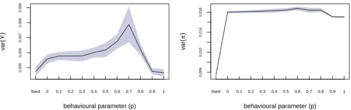
In order to stress the critical role of market sentiment in the emergence of those
fluctua-tions, Figure3contrasts the macroeconomic volatility under the baseline scenario by varying
the strength of animal spirits, i.e. the probability p of following the majority opinion, with the volatility obtained with fixed behaviour (i.e. inSeppecher(2012)). The introduction of differ-entiated behaviour for optimistic and pessimistic agents, but without animal spirits (p = 0), gives rise to significantly larger fluctuations than under the previous versions of the model
with fixed behaviour. This is especially salient for inflation (see also Figure 2c). However,
animal spirits are clearly at the roots of the emergence of large fluctuations reported in Figure
2a: the higher p, the stronger the macroeconomic volatility, especially for GDP (under the
baseline calibration, p = 0.7).
3.2.2 The deleveraging crisis along the business cycle
Figure 2a displays six phases along a typical business cycle in the model. (i) The economy
lies in the corridor of stability; (ii) an economic downturn takes place (red points), in which profits decrease, unemployment rises and inflation slows down until deflation; (iii) the economy bottoms out (see the bottom left part of the figure), deflation and unemployment are at a maximum level, and the profit share reaches a minimum; (iv) the economy starts to recover (see blue part of the loops), inflation becomes positive again, unemployment decreases, and profits start increasing again; (v) the recovery goes on, the economy experiences a boom with high inflation and low unemployment, and profits go back at their "normal times" level; and (vi) the economic activity starts slowing down, inflation decreases, and the economy settles down back in the corridor of stability.
A key point is to understand what triggers the economic downturn at step (ii). To see this
more clearly, Figure 4reports a baseline simulation. Animal spirits create contagion effects
between optimistic and pessimistic agents, which result in endogenous waves of pessimism and
optimism (avalanches), as displayed in Figure4a. Figure4bshows how each wave of pessimism
suddenly triggers a decrease in the firms’ leverage.12 This sudden mass deleveraging turns
small fluctuations into deep recessions (see Figure4c).
We stress that these abrupt opinion avalanches are an endogenous product of the model. There is no exogenous shock to trigger these rises in pessimism, and the following deleveraging crises. What happens can be understood as follows. During stable phases, the economy is characterized by small fluctuations that stem from the stochastic elements of the model (adjustments of the behaviour of the agents, matching in the markets). Most agents are optimistic and have low objectives of savings and net wealth, the share of pessimistic agents
fluctuates at low levels (see Figure 4a). These pessimistic agents have a high target of net
wealth and a high target of savings, but as long as they remain a minority, this is not enough to affect aggregate activity. However, occasionally, these pessimistic agents "contaminate" enough optimistic agents though the animal spirit component of the opinion dynamics model for the resulting deleveraging and increase in saving to affect aggregate activity. The higher
probability p, the more likely this contagion effect.13 These switches between optimism and
pessimism are endogenous and unpredictable, as they result from the complex interactions between firms’ and households’ market sentiment, their individual financial behaviour, and 12The households’ saving rate does not rise with pessimism (see Figure4b) because of the so-called Keynesian
paradox of thrift: as households are budget-constrained, attempts to build up more precautionary savings result in a decrease in aggregate demand and, in turn, incomes, so that the actual saving rate does not increase despite efforts to save more. Business cycles are therefore mostly driven by firms’ debt behaviour. Additional simulations (available upon request) where only firms or only households are subject to animal spirits, confirm this statement.
13This sudden change recalls the "Minsky moment", in reference to H. Minsky, who extensively discussed the
key role of subjective views about leverage and debt dynamics in the recurring cycles of economic instability (Minsky(1986)). See alsoBiondi(2013).
the resulting aggregate dynamics.14 Even if the alternating pattern of stability and recessions is a robust feature of the model, different simulations exhibit switches between these different regimes at different times, and with different orders of magnitude.
As a result of a sudden rise in pessimism, we observe a deleveraging crisis (Eggertsson
& Krugman (2012)). Consumption expenses, debt and dividends decrease. The velocity of circulation slows down, as bank loans are paid off and consumption expenditures decrease, and this causes a fall in prices and profits. This contributes to slow down aggregate activity, so that the pessimistic views turn out to be self-validating. This aggregate slowdown further propagates pessimistic views, as unemployment rises and sales fall, and reinforces the wave
of pessimism.15 This self-reinforcing loop drives the economy towards a deep recession (step
(iii)). The trio market sentiment/financial behaviour/aggregate dynamics forms a positive feedback system.
[Figure 4 about here.]
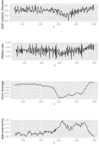
Interestingly, what follows a deleveraging crisis closely echoes what was first described as
the debt-deflation theory of Great Depressions by Fisher (1933). Paradoxically, a stronger
effort of deleveraging increases the burden of the debt (i.e. the amount of debt in real terms). This is because the aggregate effect of such a deleveraging process is an economic downturn and a fall in prices, so that deflation actually sharpens the debt burden of these firms. This
is illustrated in Figure 5, which displays a typical run where a deleveraging crisis occurs
around period 225, as the graph of firms’ leverage clearly shows (bottom panel). GDP drops, and so does inflation (expressed here in monthly rate, see middle panel). The debt’ burden increases, and picks around period 260, which corresponds to a sustained period of deflation. The second peak around period 320 also corresponds to a severe drop in prices. When the economy recovers, after period 320, inflation stabilizes at low and positive values, and the debt’ burden falls back to its pre-crisis level.
[Figure 5 about here.] 3.2.3 What drives the recovery?
After bottoming out (see step (iii)), the economy starts to recover (step (iv)). To complete
our analysis, a major point is to identify the main factors behind this recovery process. Koo
(2011) provides an explanation of the recovery after a debt-deflation cycle: "the economy
enters a deflationary spiral because, in the absence of people borrowing and spending money, the economy continuously loses demand equal to the sum of savings and net debt repayments. This process will continue until either private sector balance sheets are repaired or the private
14See alsoKirman(1993) for a similar discussion.
15This type of feedback is very similar to the dynamics of contagion models, where the probability of
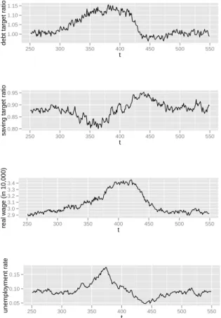
sector has become too poor to save " (Koo(2011, pp. 21-22)). However, we analyse a typical
run of the baseline scenario, and a close look at Figure6shows that the recovery starts before
the firms have achieved their objective of decrease of leverage and households have achieved their objective of savings: unemployment starts decrease around period 370, while the ratio between the firms’ debt and their target is still much higher than one, and keeps on increasing (meaning their leverage exceeds their objective, and their level of debt increases, despite their efforts to deleverage).
[Figure 6 about here.]
What actually drives the recovery in our model seems to be the increase in real wages up to the point it offsets the effect of the rise in unemployment on aggregate demand. Recall our ABM allows for both prices and nominal wages rigidities but, under our baseline calibration, nominal wages appear less flexible than prices, so that prices fall quicker than nominal wages
do, and the real wage increases. This is clearly illustrated by Figure 6 (third panel): real
wages continuously increase after the deleveraging crisis roughly from period 300 to period 420, while unemployment peaks around period 370, and then decreases to its pre-crisis level until period 420. Around period 420, the economic downturn is over, real wages decrease back to their long run level, the economy transitory overshoots its pre-crisis level (step (v)) and quickly settles down back to its stable, long-run path (step (vi)). Only after this wage-driven recovery start firms successfully deleveraging, and quickly reach their debt target, in the wake of the recovery (roughly between periods 410 and 430). Once the economy starts recovering, some firms and households turn optimistic, because unemployment decreases and sales improve and, as a result, consumption expenditures, dividends and debt start increasing again. A virtuous circle through optimism initiates in an exact symmetric way to the spiral down along a recession through pessimism.
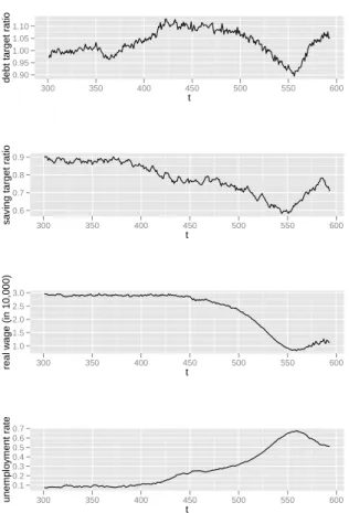
3.3 Wage flexibility in an alternative scenario
In order to demonstrate the critical role of wage rigidity in the recovery, we analyse an
alter-native scenario with more flexible nominal wages. In this scenario, we set ηH, the parameter
of wage adjustment of the households (see Equation (2)), equal to 0.25 instead of 0.05 in the
baseline scenario.16 Figure 7displays the outcomes of such a simulation (to be contrasted
with Figure6of the baseline simulation).
In the alternative scenario, households adjust downward their reservation wage faster when unemployed than in the baseline scenario. Consequently, nominal wages fall more quickly than prices, so that real wages continuously decrease after a deleveraging crisis (roughly at
period 350 on Figure 7), and a recovery driven by a rise in private consumption like in the
16The behaviour of the model is quite stable for lower than 0.25 values of η
H. Alternatively, we could have
baseline scenario is ruled out. With more flexible nominal wages, the crisis alters the income distribution in favour of profits. This in turn improves firms’ financial health, and allows them
to reach their deleverage objective in the short run (see on Figure7how the ratio of debt over
target decreases, even below unity, in the wake of the crisis, until period 370). However, this is
only a short-run effect (around 20 periods on Figure7): the decrease in real wage and, hence,
aggregate demand yields to a fall in prices, and the leverage of the firms quickly increase their target through the Fisher effect (roughly around period 370). An increasing number of them goes bankrupt, so that the share of doubtful debt increases even though the total amount of debt decreases. Even if we observe a beginning of a recovery after period 550, this is too late
for the bank, it goes bankrupt and the simulation breaks off due to a systemic crisis.17
[Figure 7 about here.]
By comparing Figures6and7, this is clear that the recession lasts roughly for 100 periods
(periods 320 to 420) in the baseline scenario, but for more than 200 periods in the alternative scenario of wage flexibility (the crisis starts around period 350, and unemployment starts decreasing again only after period 550). Moreover, unemployment reaches much higher levels under the alternative scenario than under the baseline one. This analysis tends to suggest that deleveraging crises may lead to much deeper and longer recessions if the crises last until private balance-sheets are repaired than in the case of a recovery driven by aggregate demand. The outcome of such a crisis seems therefore to depend on the way the crisis affects prices relatively to nominal wages.
3.4 Elements for policy discussion
Designing policy intervention in the Jamel model is beyond the scope of this paper, but this stage of our analysis suggests several elements to discuss potential policy intervention in face of deleveraging crises and the following recessions. Our model shows two ways out of these recessions: either by fostering aggregate demand or by repairing firms’ balance sheets. If, as the comparison between the baseline and the alternative scenarios would suggest, the first way out is faster and less costly in terms of employment, there may be room for counter-cyclical policies in sustaining aggregate demand if, in real economies, private consumption is not strong enough, or nominal wages are not rigid enough to allow for such an increase in real wage and a recovery process. In case of deep recessions with falling prices, standard monetary policy rules hit the zero lower bound of the nominal interest rate, and turn out to be powerless. However, in such cases, fiscal policy, in the form of a temporary rise in government purchases 17This is the reason why the simulation displayed in Figure7stops around period 600, and unemployment
reaches unrealistically high levels. This is due to the simple modelling of the banking sector in the current version of the ABM, which abstracts, notably, from governments or central bank’s intervention. Note that such a systemic crisis is a robust feature of the alternative scenario, as all the simulations that we have run prematurely stop after the first deleveraging crisis.
for instance, can substitute to private consumption and foster output while private agents
(firms in our model) repair their balance sheets (see Eggertsson & Krugman (2012)). As in
our model expenditures depend directly (at least partly) on income, Ricardian equivalence does not hold, and the fiscal multiplier in periods of recession is most likely higher than one.18 Demand-oriented policies can also sustain aggregate demand, and make the recovery faster.
For instance,Seppecher(2012) discusses how a minimum wage level can prevent the real wage
from falling in case of deflation, and help stabilize the economy.
Based on our model, discussing the role of monetary policy is less clear-cut. Two types of monetary policies are usually discussed in face of deep recessions with deflationary risk. On the one hand, unconventional policies, like mass purchase of private assets, could help distress firms’ balance sheets, and prematurely stop the deleveraging process and the ensuing recession. Our analysis suggests that it might be not sufficient, because sustaining aggregate demand appears as the crucial condition of the severity of the crisis, and the speed of recovery. On the other hand, the economic debate has stressed the possibility of a way out from a debt
deflation path though a rise in inflation and inflation expectations (see e.g. Blanchard et al.
(2010)). Inflation is likely to help the recovery through at least three channels. First, a rise in price may overcome wage rigidity, so that real wage falls and so does unemployment. This is the typical supply channel at work in most DSGE models but it implies that wage earners
end up paying the price of the adjustment (see, e.g., Calvo et al.(2013)). Second, besides
this demand effect, inflation may foster the recovery through the Fisher effect, by eroding the burden of the debt and help private agents to repair their balance-sheets and debtors to spend more. According to our analysis, if the recovery is preferable if wage-driven, inflation may instead erode the purchasing power of households and worsen the crisis. On the other hand, falling prices among the debt-deflation path do not raise demand, they simply intensify the
Fisher effect (see Figure5). Whether this negative demand effect or the positive Fisher effect
would dominate depends also on the origins of inflation. Our analysis suggests notably that inflation through the wage bill may foster the recovery, while inflation though higher firms’ mark-up may worsen the recession. Third, an increase in inflation decreases the real interest rate, and the cost of credits. Our model overlooks households’ debt and firms’ investment in capital, so we cannot conclude much on this point, but a credit-driven recovery could be a
useful channel to get out from the debt-deflation path (see Calvo et al.(2013) for a detailed
analysis).
18This element is similar to the effect in DSGE models with rule-of-thumb consumers, see e.g. Galí et al.
4 Conclusion
We develop a macroeconomic agent-based model which exhibits several interesting features. First, it is a model of a fully decentralized economy, in which prices and wages, and the result-ing income distribution are endogenous. Second, the model is stock-flow consistent, so that it accounts for the interdependency of all agents’ balance sheets. Third, animal spirits propagate market sentiment – i.e. optimism or pessimism – through a contagion model between agents, who, in turn, adapt their financial behaviour to their market sentiment. Financial behaviour then affect aggregate dynamics, which partly determines agents’ market sentiment. As a re-sult, the model is a positive feed-back system formed by the trio market sentiment/financial behaviour/aggregate dynamics. The emerging dynamics alternates between periods of stability and occasional big economic downturns that arise endogenously, without exogenous shocks.
In our model, economic downturns are characterized by a Fisherian debt-deflation pattern. Importantly, our simulations suggests that the end of those recessions critically depends on the way the debt-deflation spiral affects income distribution and the dynamics of prices and nominal wages. If prices fall quicker than nominal wages do, real wages increase, so that a demand-driven recovery is made possible. This recovery occurs well before the deleveraging process of firms is completed. On the contrary, if nominal wages fall faster than prices do, real wages decrease along a debt-deflation path, and a demand-driven recovery is no longer possible. The relative rise in profits improves firms’ margins, and allows them to get closer to their deleveraging objective, which may create the conditions of a recovery. However, the recession appears much deeper and longer in comparison to the demand-driven recovery. This analysis suggests that there could be significant room for counter-cyclical monetary and fiscal policies to dampen the effects of such crises. We provide some elements of policy discussion. This constitutes an immediate extension of the model, that is left for future research.
References
Akerlof, G. & Shiller, R. (2009), Animal Spirits: How Human Psychology Drives the Economy, and Why It Matters for Global Capitalism, Princeton University Press.
Allen, T. W. & Carroll, C. (2001), ‘Individual learning about consumption’, Macroeconomic Dynamics5, pp. 255 – 271.
Artus, P. (2013), Pessimisme des francais : peut-on l’expliquer par les chiffres ?, Technical report, Recherche Economique Natixis.
Baxter, M. & King, R. (1999), ‘Measuring business cycles: Approximate bandpass filters’, The Review of Economics and Statistics81(04), 575–593.
Biondi, Y. (2013), ‘Hyman Minsky’s Financial Instability Hypothesis and the Accounting Structure of Econ-omy’, Accounting, Economics and Law3(3), 141–166.
Blanchard, O., Dell’Ariccia, G. & Mauro, P. (2010), Rethinking Macroeconomic Policy. IMF Staff Position Note, janvier.
Bouchaud, J.-P. (2013), ‘Crises and Collective Socio-Economic Phenomena: Simple Models and Challenges’, Journal of Statistical Physics151(3-4), 567–606.
Brock, W. A. & Hommes, C. H. (1997), ‘A Rational Route to Randomness’, Econometrica65(5), 1059–1096. Burdett, K. & Vishwanath, T. (1988), ‘Declining Reservation Wages and Learning’, The Review of Economic
Studies55(4), 655–665.
Calvo, G. (1983), ‘Staggered prices in a utility maximizing framework’, Journal of Monetary Economics12, pp. 383–398.
Calvo, G., Coricelli, F. & Ottonello, P. (2013), Jobless Recoveries During Financial Crises: Is Inflation the Way Out?, NBER Working Papers 19683, National Bureau of Economic Research, Inc.
Carroll, C. D., Dynan, K. E. & Krane, S. D. (2003), ‘Unemployment Risk and Precautionary Wealth: Evidence from Households’ Balance Sheets’, The Review of Economics and Statistics85(3), 586–604.
Carroll, C., Fuhrer, J. & Wilcox, D. (1994), ‘Does Consumer Sentiment Forecast Household Spending? If So, Why?’, American Economic Review84(5), 1397–1408.
Caverzasi, E. & Godin, A. (2013), Stock-flow consistent modeling through the ages, Technical report, Working Paper, Levy Economics Institute.
Clauset, A., Shalizi, C. & Newman, M. (2009), ‘Power-law distributions in empirical data’, SIAM Review 51, 661–703.
Clementi, F. & Gallegati, M. (2005), ‘Power law tails in the italian personal income distribution’, Physica A 350, 427–438.
Cyert, R. & March, J. (1963), A Behavioral Theory of The Firm, Prentice-Hall, Englewood Cliffs, New Jersey. Dawid, H., Gemkow, S., Harting, P., van der Hoog, S. & Neugart, M. (2014), Agent-Based Macroeconomic Modeling and Policy Analysis: The Eurace@Unibi Model, Technical Report 01-2014, Bielefeld Working Papers in Economics and Management.
De Grauwe, P. (2011), ‘Animal spirits and monetary policy’, Economic Theory47, 423–457. De Grauwe, P. (2012), Lectures on Behavioral Macroeconomics, Princeton University Press.
Delli Gatti, D., Desiderio, S., Gaffeo, E., Cirillo, P. & Gallegati, M. (2010), Macroeconomics from the Bottom-Up, Springer.
Delli Gatti, D., Gallegati, M., Greenwald, B., Russo, A. & Stiglitz, J. E. (2010), ‘The financial accelerator in an evolving credit network’, Journal of Economic Dynamics and Control34(9), 1627–1650.
Dosi, G., Fagiolo, G., Napoletano, M. & Roventini, A. (2013), ‘Income distribution, credit and fiscal policies in an agent-based keynesian model’, Journal of Economic Dynamics & Control . (accepted manuscript). Dosi, G., Fagiolo, G. & Roventini, A. (2010), ‘Schumpeter Meeting Keynes: A Policy-Friendly Model of
Endogenous Growth and Business Cycles’, Journal of Economic Dynamics and Control34(9), 1748–1767. Eggertsson, G. B. & Krugman, P. (2012), ‘Debt, deleveraging, and the liquidity trap: A fisher-minsky-koo
Fisher, I. (1933), ‘The debt-deflation theory of Great Depressions’, Econometrica1(4), 337–357.
Fuhrer, J. (1995), ‘The persistence of inflation and the cost of disinflation’, New England economic review pp. 3–16.
Fujiwara, Y. (2003), ‘Zipf law in firms bankruptcies’. http://arxiv.org/archive/condmat/0110062.
Galí, J., López-Salido, D. & Vallés, J. (2007), ‘Understanding the Effects of Government Spending on Con-sumption’, Journal of the European Economic Association, MIT Press5(1), 227–270.
Gallegati, M., Giulioni, G. & Kuchiji, N. (2003), ‘Complex Dynamics and Financial Fragility in an Agent-Based Model’, Advances in Complex Systems6, 267–282.
Geanakoplos, J. (2010), ‘Solving the present crisis and managing the leverage cycle’, Economic Policy Design 16(1).
Hackbarth, D. (2009), ‘Determinants of corporate borrowing: A behavioral perspective’, Journal of Corporate Finance15, 389–411.
Hauenschild, N. & Stahlecker, P. (2001), ‘Precautionary saving and fuzzy information’, Economics Letters 70, 107–114.
Hommes, C. (2011), ‘The heterogeneous expectations hypothesis: Some evidence from the lab’, Journal of Economic Dynamics and Control35(1), 1–24.
Keynes, J. (1936), The General Theory of Employment, Interest and Money, Palgrave Macmillan. Kimball, M. (1990), ‘Precautionary saving in the small and in the large’, Econometrica58, 53–73.
Kirman, A. (1993), ‘Ants, Rationality, and Recruitment’, The Quarterly Journal of Economics108(1), 137–56. Koo, R. C. (2011), ‘The world in balance sheet recession: causes, cure, and politics’, Real-world economics
review58, pp. 19–37.
Leijonhufvud, A. (2009), ‘Out of the Corridor: Keynes and the Crisis’, Cambridge Journal of Economics 33(4), 741–757.
Lengnick, M. (2013), ‘Agent-based macroeconomics – a baseline model’, Journal of Economic Behavior & Organization86, 102–120.
Lux, T. (1995), ‘Herd Behaviour, Bubbles and Crashes’, Economic Journal105(431), 881–96.
Lux, T. (1998), ‘The socio-economic dynamics of speculative markets: interacting agents, chaos, and the fat tails of return distributions’, Journal of Economic Behavior & Organization33(2), 143–165.
Minsky, H. (1986), Stabilizing an Unstable Economy, Yale University Press.
Reed, W. J. (2003), ‘The Pareto law of incomes – an explanation and an extension’, Physica A319, 469–486. Riccetti, L., Russo, A. & Gallegati, M. (2012), An agent-based decentralized matching macroeconomic model.
Università Politecnica delle Marche, Ancona, Italy.
Seppecher, P. (2012), ‘Flexibility of wages and macroeconomic instability in an agent-based computational model with endogenous money’, Macroeconomic Dynamics16(2), 284–297.
Sharpe, S. A. (1994), ‘Financial Market Imperfections, Firm Leverage, and the Cyclicality of Employment’, The American Economic Review84(4), 1060–1074.
Simon, H. (1955), ‘A behavioural model of rational choice’, Quarterly Journal of Economics69, pp. 99–118. Simon, H. (1962), The architecture of complexity, in ‘Proceedings of the American Philosophical Society’, Vol.
106, pp. 467–481.
Sornette, D. (2003), Why stock markets crash, Princeton University Press.
Stock, J. & Watson, M. (1999), Business Cycle Fluctuations in U.S. Macroeconomic Time Series, in J. Taylor & M. Woodford, eds, ‘Handbook of Macroeconomics’, Elsevier Science: Amsterdam.
Tedeschi, G., Iori, G. & Gallegati, M. (2012), ‘Herding effects in order driven markets: The rise and fall of gurus’, Journal of Economic Behavior & Organization81(1), 82–96.
Tesfatsion, L. (2006), Agent-based computational economics and macroeconomics, in D. Colander, ed., ‘Post Walrasian Macroeconomics: Beyond the Dynamic Stochastic General Equilibrium Model’, Cambridge Uni-versity Press, chapter 16, pp. 175–202.
Vriend, N. (2000), ‘An illustration of the essential difference between individual and social learning, and its consequences for computational analyses’, Journal of Economic Dynamics and Control24, 1–19.
Windrum, P., Fagiolo, G. & Moneta, A. (2007), ‘Empirical Validation of Agent-Based Models: Alternatives and Prospects’, Journal of Artificial Societies and Social Simulation10(2), 8.
consumption employment inflation change in inventories velocity of money vacancy rate −1.0 −0.5 0.0 0.5 1.0 t−12 t−8 t−4 t t+4 t+8 t+12
(a) Cross-correlation with GDP at time t (pro-cyclical variables)
unemployment unemployment duration share of doubtful debts
−1.0 0.0 0.5 1.0 t−12 t−8 t−4 t t+4 t+8 t+12
(b) Cross-correlation with GDP at time t (contra-cyclical variables)
t−4 t−8 t−12 t−18 t−24 0.0 0.2 0.4 0.6 0.8 (c) GDP autocorrelation func-tion t−4 t−8 t−12 t−18 t−24 0.0 0.1 0.2 0.3 0.4 (d) GDP autocorrelation func-tion 200 400 600 800 1000 1200 2 4 6 8 10 period KF KB
(e) Capital ratio (bank over firms)
10 20 30 40 50 60 −5 0 5 10 Unemployment Profits/Wages Inflation
(a) Baseline scenario
0 10 20 30 40 50 60 −10 0 10 Unemployment Profits/Wages Inflation
(b) Fixed behaviour (Seppecher
(2012)) 0 10 20 30 40 50 60 −10 0 10 Unemployment Profits/Wages Inflation
(c) Baseline scenario without animal spirits (p = 0)
Figure 2: Co-evolution of unemployment, income distribution (Profits/Wages) and inflation during the business cycle in the model with the Jamel model. Each point represents a period during a simulation. Numbers are percentages.
0.005 0.006 0.007 0.008 0.009 behavioural parameter (p) v ar ( Y ) fixed 0 0.1 0.2 0.3 0.4 0.5 0.6 0.7 0.8 0.9 1 0.006 0.010 0.014 0.018 behavioural parameter (p) v ar ( π ) fixed 0 0.1 0.2 0.3 0.4 0.5 0.6 0.7 0.8 0.9 1
Figure 3: Average volatility of output gap (left panel) and inflation (right panel) over 30 replications of the simulations, 1, 400 periods (the grey bands give the standard deviation), for different behavioural assumptions ("fixed" corresponds to the model with fixed behaviour inSeppecher(2012))
(a) Share of pessimistic agents (b) Precautionary behaviour (c) Real GDP and consumption
350 400 450 500 150 200 250 300 350 t GDP (v olume , thousands) −0.01 0.00 0.01 0.02 150 200 250 300 350 t inflation r ate 0.62 0.64 0.66 0.68 0.70 0.72 150 200 250 300 350 t fir ms' le v er age 1.60 1.65 1.70 1.75 1.80 150 200 250 300 350 t
debt (real ter
ms)
Figure 5: Illustration of the evolution of debt and GDP during a deleveraging crisis (around period 225)
1.00 1.05 1.10 1.15 250 300 350 400 450 500 550 t debt target r atio 0.80 0.85 0.90 0.95 250 300 350 400 450 500 550 t sa ving target r atio 2.9 3.0 3.1 3.2 3.3 3.4 250 300 350 400 450 500 550 t real w age (in 10,000) 0.05 0.10 0.15 250 300 350 400 450 500 550 t unemplo yment r ate
Figure 6: Illustration of the evolution of firms’ debt and households’ savings (both expressed as a ratio over the targeted level) and real wage in a typical run of the baseline scenario – deleveraging crisis around period 300
0.90 0.95 1.00 1.05 1.10 300 350 400 450 500 550 600 t debt target r atio 0.6 0.7 0.8 0.9 300 350 400 450 500 550 600 t sa ving target r atio 1.0 1.5 2.0 2.5 3.0 300 350 400 450 500 550 600 t real w age (in 10,000) 0.1 0.2 0.3 0.4 0.5 0.6 0.7 300 350 400 450 500 550 600 t unemplo yment r ate
Figure 7: Illustration of the evolution of firms’ debt and households’ savings (both expressed as a ratio over the targeted level) and real wage during a crisis in the alternative scenario