On the performance of UNB for Machine-To-Machine Low Earth Orbit (LEO) satellite communications

HAL Id: hal-03012552

https://hal.archives-ouvertes.fr/hal-03012552

Submitted on 20 Nov 2020

HAL is a multi-disciplinary open access

archive for the deposit and dissemination of

sci-entific research documents, whether they are

pub-lished or not. The documents may come from

teaching and research institutions in France or

abroad, or from public or private research centers.

L’archive ouverte pluridisciplinaire HAL, est

destinée au dépôt et à la diffusion de documents

scientifiques de niveau recherche, publiés ou non,

émanant des établissements d’enseignement et de

recherche français ou étrangers, des laboratoires

publics ou privés.

To cite this version:

Mehdi Anteur, Nathalie Thomas, Vincent Deslandes, André-Luc Beylot. On the performance of UNB

for Machine-To-Machine Low Earth Orbit (LEO) satellite communications. International Journal of

Satellite Communications and Networking, Wiley, 2019, 37 (1), pp.56–71. �10.1002/sat.1285�.

�hal-03012552�

Correspondence

Nathalie Thomas, IRIT Lab, University of Toulouse, Toulouse, France.

Email: nathalie.thomas@enseeiht.fr

attractive for satellite communications but also draw new challenges compared with terrestrial systems where this technology is already deployed. Indeed, the main advantage of UNB signals, their small bandwidth, makes them more sensitive to frequency drifts that are particularly present in the case of LEO satellite systems. It also implies the use of a random access method in which the carrier frequency is a parameter unknown by the receiver. In this paper, we propose a general semianalytical model to evaluate the performance of a terrestrial or satellite system using UNB technology, taking into account the multiuser interference and the frequency drift. This model is then used to assess the performance (packet loss ratio and throughput) on the return link medium access control (MAC) of a representative LEO satellite system. With our model, we analyze the effect of frequency drift on the system performance. This paper also proposes to investigate more deeply the multiuser interference modeling in order to estimate accurately the performances of a UNB system in terms of bit error rate (BER). We propose a semianalytical approach to study the interference in presence of arbitrary power imbalance that includes the effect of frequency offset and frequency drift and applicable for any linear modulation and any pulse-shaping filter. The expression of the multiuser interference is established in the general case. We then propose a methodology to compare this exact model to the Gaussian interference approximation (mainly used through the central limit theorem) in order to assess its accuracy.

KEYWORDS

Aloha, doppler effect, IoT, M2M, satellite, UNB

1

INTRODUCTION

Machine-to-machine (M2M)1,2_{covers communications between devices that do not require direct human intervention. Although they have long} existed, the services made possible by this type of communications are rapidly expanding and are one of the most dynamic markets in the information technology sector. The satellite field contributes to the growth of this promising market. Various M2M systems are operational or in preparation, offering the prospects of M2M systems with global coverage. Most of them, such as Orbcomm, Iridium, Globalstar, or Argos, use a low earth orbit (LEO) satellite constellation.3

Among the variety of M2M applications, a new type of need is clearly emerging for very cheap service (< 10$ per year) on cheap terminal devices (< 10$) with very long autonomy (years with a single AA battery) and long range (> 10 km), for the transmission of very small-sized uplink messages (< 100 bytes).3_{A lot of examples could be given; the monitoring of devices by manufacturers to diagnose problems is a well-known} one. Existing communication systems are not well suited to this new type of need. Sensor-oriented protocols (as ZigBee, Z-Wave, and Wibree), used in wireless personal area networks (WPAN), are not suitable for sending traffic at long range. In contrast, wireless wide area networks (WWAN) or cellular networks (as GPRS, UMTS, and LTE) offer a rich variety of long-range high data rate services but are not designed for the transmission of small messages for low consumption terminals (autonomy for a single battery in the order of days, not years). Thus, low-power wide-area (LPWA) communication systems have been introduced.

systems where, because of high satellite velocities (several kilometers per second), the Doppler rate is in the order of hundreds of hertz per second, which is in the same order of magnitude as a UNB signal bandwidth. An example of UNB signals, received from a satellite at an altitude of 720 km, is represented on Figure 1. The maximum Doppler rate is −100 Hz/s for a carrier frequency of 400 MHz or −700 Hz/s for a carrier frequency of 3 GHz (the values are negative because the frequency shift is decreasing as the satellite passes by).

Regarding access methods, classical frequency division multiplexing access (FDMA) techniques are not adapted for UNB transmissions. Indeed, it is not possible to reach the needed level of precision in synchronization (eg, few hertz for a 100-Hz channel) with low-cost electronic components embedded in end terminals. Thus, the use of UNB signals implies a random access (RA) method in which the carrier frequency is a parameter unknown by the receiver. There are many RA techniques proposed in the literature.5-10_{We will focus in our study on extended} versions of Aloha for UNB signals, which we call time/frequency Aloha (TFA) for asynchronous transmissions and slotted TFA (STFA) when UNB message transmissions are synchronized in time: See Figure 2. In both cases, the frequency is chosen randomly within a specific bandwidth.

Currently, no model can be used to assess system performance in a UNB system with frequency drift. del Ro Herrero and De Gaudenzi11 and all the reference therein propose a general framework to study the performance of random access schemes for system using forward error correction (FEC) and taking into account power imbalance. This model is more general than any previous model, but it relies on a Gaussian interference approximation, which does not hold well for asynchronous UNB signals (see Section 4.3). An attempt has been made in Do et al12_to model multiuser interference for UNB signals, but the model is restricted to iso-power BPSK signals without FEC. In our contribution, we propose a semianalytical model that applies for many Aloha-based random access schemes, and which supports arbitrary power distribution, frequency drift, and FEC. This model relies on the definition of a vulnerability area in which the message, or packet, of interest can interfere with other ones (see Figure 3 representing a zoom on Figure 1). This allows to compute the probability of collision and then estimate the packet loss ratio (PLR) and the throughput for the UNB transmission.

FIGURE 1 Example of multiple UNB signals received by a LEO satellite [Colour figure can be viewed at wileyonlinelibrary.com]

FIGURE 3 Time/frequency detection in white, time/frequency/frequency drift detection in black on two UNB signals with frequency drifts of −400 and −200 Hz/s [Colour figure can be viewed at wileyonlinelibrary.com]

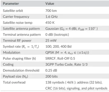
TABLE 1 Main system parameters

Parameter Value

Satellite orbit 700 km Carrier frequency 1.6 GHz Satellite noise temp 450 K

Satellite antenna pattern Gaussian (G0= 4 dBi, 𝜃3dB= 110◦)

Terminal antenna pattern 0 dBi (isotropic) Terminal RF power 25 mW Symbol rate (Rs = 1∕Ts) 100, 200, 400 Bd

Modulation QPSK (M = 4, an,k∈ {±1±j})

Pulse shaping filter (h) SRRCF, Roll-Off 0.5 Coding 3GPP Turbo Code, Rate 1/3 Demodulation threshold 0.25 dB

Payload size (Nb) 200 bits

Total overhead 138 symbols ( 46% ): address (32 bits), CRC (16 bits), signaling, and pilot symbols

To accurately investigate the bit error rate (BER) performance, the effect of packets' carrier frequency offset on the system capacity has to be taken into account but is not so trivial, because, on the one hand, it increases the number of collision, but on the other hand, the collisions are less destructive since two interfering messages are rarely completely overlapping. Even if the interference can be generated by simulating a full system, it could be tedious to implement multiple systems and compare them, hence the need of simple, easy to use, and accurate interference modeling. The main difficulty is to evaluate the probability density function (PDF) of the multiuser interference, and even though it is possible to derive it in some specific scenarios (for instance, the PDF of BPSK interferer with rectangular pulse shaping is given in previous studies13-16_{) in the} general case, it is not easy to derive it in a tractable form. Another approach is to approximate it with a known distribution and fitted parameters. In this paper, we propose a semianalytical approach to study the interference in presence of arbitrary power imbalance that includes the effect of frequency offset and frequency drift and applicable for any linear modulation and any pulse shaping filter. The expression of the multiuser interference is derived in the most general case. We then propose a methodology to compare this exact model to the Gaussian interference approximation (GIA), mainly adopted in virtue of the central limit theorem, in order to assess its accuracy.

The rest of the paper is organized as follows. In Section 2, we describe the system under consideration and how it is modeled. In Section 3, we describe the semianalytical model used to evaluate its random access performance. In Section 4, an exact model of the multiuser interference is derived and used to compare with Gaussian interference approximation in terms of obtained bit error rates. Finally, some conclusions are drawn in Section 5.

2

SYSTEM MODELING

The system under consideration is a LEO mobile satellite system operating in L band, able to provide a global coverage and an uplink traffic to millions of low-power and low-cost M2M terminals. The satellite has a single antenna beam on which it transmits a beacon to indicate its presence to the terminals. Terminals in visibility may then transmit their message to the satellite. On the ground, terminals are considered uniformly distributed and transmitting small-sized packets, low data rate, and low duty cycle traffic packets using UNB signals. The aggregate

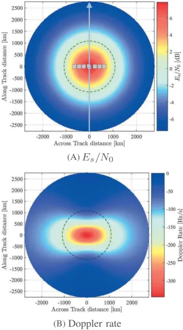
FIGURE 4 Physical parameters of the signal received as a function of the positions of the users under the satellite coverage. The dashed line represents the satellite radio visibility (Es∕N0 > 0.25 dB) and the whole surface represents the geometrical visibility [Colour figure can be

viewed at wileyonlinelibrary.com]

traffic is modeled as a Poisson arrival process. All terminals are assumed to use one of the following Aloha-based random access scheme, namely, pure Aloha (PA, the users send their messages at the same frequency and at any random times), slotted Aloha (SA, the time is chosen within a discrete set of values; the frequency is the same for all users), time/frequency Aloha (TFA, time is random, and the frequency is chosen randomly within a specific bandwidth), or slotted TFA (STFA, the time is chosen within a discrete set of values; the frequency is chosen randomly within a specific bandwidth). Figure 2 summarizes these different random access schemes with and without frequency drifts.

Let us call sn(t) the complex envelop associated to a transmitted message (terminal number n). It can be written as

sn(t) = N_∑s−1

k=0

an,kh(t − kTs), (1)

where an,krepresents the kth complex symbol of the nth user and is taken in the modulation M-ary alphabet. h is the pulse shaping filter impulse

response, Ts= _R1

s

is the symbols period, and Nsis the number of symbols in each considered burst.

Each of the snsignals goes through a different channel that consists of an amplitude factor An(including transmit power, free path loss and

fading), a delay 𝜏n(including asynchronism between users and the propagation delay), a phase offset 𝜙n(asynchronism between the users and

the receiver and channel), a frequency shift fnrelative to the carrier frequency (caused by the access method and the Doppler effect), and a

frequency drift dn(assumed to be caused by the Doppler rate only). All of the parameters are independent between users, but for a specific user,

the parameters might not be independent. For instance, in a system without power control when the delay is high (long distance), the amplitude is low (high free space loss). Without loss of generality, we can assume that the receiver is synchronized on the useful signal; let us say s0(t),

FIGURE 5 Marginal distribution of the Doppler rate (left) and of Es∕N0(right) [Colour figure can be viewed at wileyonlinelibrary.com]

The complex envelope of the received signal r(t) can be written as

r(t) =

L

∑

n=0

Anrn(t) + n(t) (2)

with n(t) being a white complex Gaussian noise of double-sided power spectral density 2N0, L the number of users, and rn(t) the complex envelope

of the signal received from the nth user defined as

rn(t) = N∑s−1 k=0 an,kh(t − kTs− 𝜏n)e j ( 𝜙n+2𝜋fn(t−𝜏n)+2𝜋dn(t−𝜏n ) 2 2 ) . (3)

Because of the asynchronism between the terminals and the satellite, 𝜙n follows a uniform distribution. Since the traffic is assumed to be

Poisson, the instant when the signal is received tn(including 𝜏n) is also uniformly distributed (in the case of slotted random access, tnis simply

discretized). The frequency shift fnwill be assumed to be uniformly distributed and independent from the other parameters since it is caused

by the random access method. We also assume that the modification of the distribution caused by the Doppler shift is compensated on the transmitter side. However, the power and the frequency drift cannot be modeled with a simple distribution since these physical parameters are not independent. Therefore, to generate these two physical parameters, we consider the point of view of a single satellite whose parameters are summarized in Table 1. We first randomly pick a point under the satellite coverage, and then we compute the physical parameters at this point. The Doppler rate and the signal to noise ratio per symbol, Es

N0

, under the satellite coverage are shown in Figure 4. We can see for instance that high Doppler rate is highly correlated to high Es

N0

. The dashed line represents the radio visibility, and the area in which the user are picked. Indeed, since terminals only transmit when the satellite beacon is detected, we consider that all the messages received by the satellite have a Es

N0

high enough to be demodulated correctly. The obtained marginal distributions of the frequency drift (denoted pdin the following) and of the_NEs

0

are illustrated on Figure 5.

3

RANDOM ACCESS FOR UNB TRANSMISSIONS

3.1

Introduction

Relying on the definition of a vulnerability area in which the message, or packet, of interest can interfere with other ones, this section proposes to estimate the packet loss ratio (PLR) and the throughput for a UNB transmission. Our semianalytical model applies for many Aloha-based random access schemes and supports arbitrary power-distribution, frequency drift, and FEC.

3.2

Performance model

The two random access performance metrics that we are interested in are the throughput or capacity (in bit/s/Hz) and the packet loss ratio (PLR). In this section, we describe the semianalytical model used in order to estimate the PLR. The throughput is linked to the PLR through the relation:

Throughput(λ) = λ(1 − PLR(λ)), (4) where λ is the average MAC load. To derive the PLR, it is assumed that the traffic is composed of packets that have the same length T and the same two-sided frequency bandwidth B. The number of transmissions within a unit time of T and frequency bandwidth of B follows a Poisson

FIGURE 6 Examples of vulnerability areas for a TFA access method, a PoI whose dn = 0, and three different interfering packets whose

frequency drifts dmare set to d1, d2, and d3[Colour figure can be viewed at wileyonlinelibrary.com]

distribution of parameter λ. Using the total probability theorem, we can express the PLR for a fixed load λ as a function of the PLR knowing the number of packets in collision:

PLR(λ) =

∞

∑

k=0

P(k, λ)PLRk, (5)

where P(k, λ) is the probability for a packet to interfere with k other packets and PLRkis the probability to lose a packet when it is interfering with

k messages.

The probability P(k, λ) for a message sn(t) (packet of interest or PoI) to interfere with k other ones ({sm(t)} , m = 1, · · ·, k with m≠ n) for a given

average MAC load λ can be expressed as the probability that the k other messages arrive within sn(t) vulnerability area. The vulnerability area is a

geometric zone in the time/frequency space in which, if a packet begins, it will overlap with the PoI. The size of the vulnerability area depends on the packet length T, the packet bandwidth B, the frequency drift dnof the PoI, the frequency drift of the messages in collision dm, m ≠ n, and on

the used access method. Note that the vulnerability area may also depend on modulation, coding, and filtering. Figure 6 represents examples of vulnerability areas for a TFA access method, a PoI whose dn = 0, and three different interfering packets whose frequency drifts are set to d1, d2,

and d3. It shows that the vulnerability area can be decomposed into two parts: a part formed by shapes of the same size as the packets (in plain

color on the figure) and a second part resulting from the presence of a difference of frequency rate (middle part in hatched grey). With simple algebra, it can be demonstrated that the size of the vulnerability area is equal to 4BT + T2_|d

n− dm| (see Section 6). It can be shown, in the same

way, that the vulnerability area would be equal to 2BT + T2_|d

n− dm| in the case of a STA access method and BT + T2|dn− dm| in the case of a SA

access method.

When the frequency drift is distributed according to a continuous pdf pd(see Section 2), P(k, λ) can be expressed as

P(k, λ) = ∫ +∞ −∞ pd(dn) (g(dn)λ)k k! exp (−λg(dn)) ddn, (6) where g(dn) = 𝛼 + T B ∫ +∞ −∞ pd(dm)|dn− dm|ddm (7)

with 𝛼 = 1 for SA, 𝛼 = 2 for PA and STFA, and 𝛼 = 4 for TFA. g(dn) representing the average number of messages interfering with a packet of

frequency drift dnfor a load of 1 Erlang. It is worth noting that when the frequency drift can be neglected (ie, when pdis the delta Dirac function),

this formula can be simplified into the well-known expression5,6_:

P(k, λ) =(𝛼λ)

k

k! e

−𝛼λ_{. (8)}

Since P(k, λ) decreases rapidly as k increases, the PLR can be approximated with a truncated sum:

PLR(λ) ≈

K

∑

k=0

P(k, λ)PLRk, (9)

where K is chosen such as∑K_k=0P(k, λ) > 1 − 10−3_{, meaning that we consider 99.9% of the possible number of colliding packets. In the studied}

scenarios and for the loads under consideration, this criterion leads to K < 80. PLRkis computed numerically using a Monte-Carlo simulation.

First, the signal of a useful packet; let us say s0(t) is generated with a set of physical parameters

{(_E s N0 ) 0 , t0, 𝜙0, f0, d0 }

. Then the signals of k interfering packets are generated with the parameters{(Es

N0

)

m, tm, 𝜙m, fm, dm

}

for m ∈ {1, .., k} in a way that leads to a collision with the useful packet. A packet is counted as lost if there is a least one erroneous bit at the output of the FEC decoder.

It is assumed that the receiver performs a perfect detection of the packets and a perfect estimation of the physical parameters of the useful signal. In a practical system, these two aspects can become challenging, and the performance results obtained in the following are therefore representing an upper bound. Detailed signal detection processing considerations are beyond the scope of this paper and will be treated in future work, but the detection could for instance be done using a multidimensional search based on preamble symbols and the frequency drift estimated with a specific algorithm (for instance, see Abatzoglou17_{and references therein). These two estimators imply an increased receiver complexity,} and some performance losses should be expected, especially in high interference conditions, nevertheless for the loads under consideration their impact is assumed to be negligible.

FIGURE 7 Frequency shift interval [fmin, fmax] that leads the interfering packet (in red) to interfere with the packet of interest (in blue) [Colour

figure can be viewed at wileyonlinelibrary.com]

To generate interfering messages, the frequency drift dmis first drawn using an arbitrary distribution. Then the instant tmis drawn, using

a uniform distribution, such as a collision occurs. For two messages to interfere, they must share the same time/frequency space. The time condition for two messages of length T to interfere is straightforward:

Δt = tm− t0∈ [−T, T]. (10)

Then the minimum and maximum values of the frequency shift (fmin, fmax) are computed for a message with starting instant tmand frequency drift

dmto interfere with the useful packet. Finally, a frequency shift value fmis drawn, using a uniform distribution, within the interval

[

fmin, fmax

] . Such bounds are represented on Figure 7 for all possible sign combinations of the time difference Δt and drift difference Ed = dm− d0. This figure

shows a schematic time-frequency representation of packets in which the packet of interest is represented in blue while interfering packets at the collision limits are represented in red. We can note that packets are represented by parallelogram instead of rectangles because of the frequency drift. Points of collision are represented green triangle (resp circle) for the minimum (resp maximum) frequency shift value. Using the Heaviside function H(x) ∀x ∈ R, H(x) = ⎧ ⎪ ⎨ ⎪ ⎩ 0 x < 0 1 2 x = 0 1 x > 0 , (11)

it is possible to write the bounds of the frequency shift in a single simple expression:

fmin(d0, dm, Δt) = d0− B + (dm− d0)H((dm− d0)Δt)Δt

− (dm− d0)H((dm− d0))T + dm− d0Δt.

(12) With the symmetry in frequency, it can be demonstrated that

fmax(d0, dm, Δt) = 2f0− fmin(−d0, −dm, Δt). (13)

Without loss of generality, we can choose t0 = 0 and f0 = 0, but no specific value can be assumed for d0since its distribution depends on the

system.

3.3

Performance analysis

The equations in the previous section enable to compute the throughput and PLR by computing two terms: PLRkand P(k, λ). In the following

paragraphs, those two terms are evaluated for the system described in Section 2 and the effect of the frequency drift is analyzed.

Figure 8 shows PLRkfor k taking values from 1 up to 50 for both TFA and STFA and for different symbol rates. It illustrates two phenomena.

First and as expected, we can observe that for the same number of interfering messages, TFA has a lower PLR than STFA. Indeed, in the slotted case, messages are aligned in time so interferences occur potentially during the full length of the packet while in the nonslotted case, only part of

FIGURE 8 PLRkas a function of the number of interfering message k [Colour figure can be viewed at wileyonlinelibrary.com]

FIGURE 9 Schematic representation of interfering messages for different symbol rate (for fixed payload size) [Colour figure can be viewed at wileyonlinelibrary.com]

the burst is affected by the interfering packet. Secondly, we can also observe that the PLR decreases with the symbol rate. This is also expected since, as the symbol rate decreases, the signal bandwidth becomes narrower and the signal length increases. Both these aspects make the effect of the frequency drift more significant since the area where messages overlap shrinks and at the same time the number of symbols involved in the collision is reduced (see Figure 9). It is worth noting that in order to do a fair comparison, the link budget is kept the same when the symbol rate is changed (this means for instance that the terminal RF transmission power decreases with the symbol rate to keep the same Es∕N0range).

However, even though the PLR difference for various symbol rates is present, it is not significant and the reduction of the PLR offered by the frequency drift can be neglected with our system parameters for Rs ≥ 400 Bd (and more generally, when the signal bandwidth becomes large

compared with the worst case frequency drift). Furthermore, as the number of interferers increases, the difference becomes less significant. Combining the probability of collision with the probability of losing a packet with (5), we obtain the overall PLR (Figure 10). The figure on top (resp bottom) shows the throughput (resp the PLR) as the function of the input load. The load λ expressed in bit/s/Hz is obtained with the following formula:

λbit∕s∕Hz= λErlang

Nb

TB, (14)

where Nbis the payload size in bits and B is the frequency bandwidth of a packet taking into account the filter roll-off.

In the commonly admitted domain of practical use (typically PLR≤ 10−1_{), the PLR performances of TFA are consistent with the performance}

obtained for the PLRk. However for STFA, the performances are reversed: The PLR is smaller for larger symbol rates. This reflects that in STFA, the

increase of collision caused by the frequency drift is not compensated by the reduction of the severity of multiple access interference. The PLR of

PA and SA, given for reference, are computed assuming a perfect synchronization and a perfect correction of the frequency drift. The throughput

is given for illustration purpose and for comparison with results in the literature only. For a PLR of 10−2_{, TFA can achieve a spectral efficiency of}

0.013 bit/s/Hz (with Rs = 100 Bd), which is +67% compared with STFA, more than two times of what PA can achieve in the same conditions

and 2.4 times the spectral efficiency of SA. These figures, even though they are an improvement over those of classical Aloha schemes, are several order of magnitude away from state of the art random access scheme such as E-SSA10_{or CRDSA.}8_{Nevertheless, the results presented} in this paper are interesting because they demonstrate that it is not necessary for a UNB transmitter using TFA to compensate for the frequency drift since the PLR is improved by it. Furthermore, these results are not limited to systems impaired by Doppler rate. They could be extended

FIGURE 10 Comparison of the throughput and PLR of PA∕SA∕TFA∕STFA with different symbol rates in presence of frequency drift [Colour figure can be viewed at wileyonlinelibrary.com]

to systems in which the frequency drift is not naturally present but voluntarily introduced in order to improve performances. It would then be possible to tailor specifically the frequency drift distribution in order to maximize the gain in performance. Our study focuses on simple random access schemes, but it would be interesting to measure the benefit of such measure on state of the art random access schemes that can achieve much higher capacity. For the study of such cases the model would show its limitation since the effect of the packet detection and the frequency synchronization would no longer be negligible. The model can also be improved to take into account different packet lengths, different symbol rates or different code rates.

4

MULTIUSER INTERFERENCE MODELING FOR UNB TRANSMISSIONS

4.1

Introduction

This section investigates more deeply into multiuser interference modeling in order to estimate accurately the performance of a UNB system in terms of bit error rate (BER). We propose a semianalytical approach to study the interference in presence of arbitrary power imbalance that includes the effect of frequency offset and frequency drift and applicable for any linear modulation and any pulse shaping filter. The expression of the multiuser interference is established in the general case. We then propose a methodology to compare this exact model to the GIA in order to assess its accuracy.

4.2

Exact interference model

The complex envelope of the received signal r(t) can be written as in Equation 2:

r(t) =

L

∑

n=0

Ψ (t, 𝜙, f, d) = ej 𝜙+2𝜋ft+2𝜋d

t2

2 _{. (17)}

At the output of the matched filter, the signal is given by

y(t) = r(t) ⊗ h∗_{(−t) = A} 0y0(t) + L ∑ n=1 Anyn(t) + w(t), (18)

where ⊗ represents the convolution product, h∗

is the complex conjugate of h, w(t) is the filtered noise, and yn(t) the complex envelope of the nth

user signal after the matched filter. The first term is considered to be the useful signal, the second term is the multiuser interference, and the last term is the filtered thermal noise. As stated in the introduction, the main difficulty is to find the distribution (pdf) of this multiuser interference term. In some specific case, it is possible to derive the exact pdf but in our general case, the task becomes very strenuous. Our approach is thus to establish a simplified expression of the interference to make its implementation friendly and then use it to run Monte-Carlo simulations. This semianalytic approach is halfway between a full implementation of the physical layer, which is more complex and a full analytical approach that is out of reach.

The nth interference signal at the output of the matched filter, y_n(t), can be expressed as

yn(t) = rn(t) ⊗ h∗(−t) = ∫ ∞ −∞ rn(x)h∗(x − t)dx = N_∑s−1 k=0 an,k_∫ ∞ −∞ h∗_{(x − kT} s− 𝜏n)h∗(x − t)Ψ (x − 𝜏n, 𝜙n, fn, dn) dx. (19)

It can be demonstrated with simple algebra that the Ψ function verifies the following relation: Ψ (x − 𝜏n, 𝜙n, fn, dn) = Ψ (x − 𝜏n− kTs+ kTs, 𝜙n, fn, dn) = Ψ ( x − 𝜏n− kTs, 𝜙n+ 2𝜋 ( fnkTs+ 1 2dn(kTs) 2 ) , fn+ dnkTs, dn ) . (20)

Using (20) and the change of variable u = x − kTs − 𝜏n, we can rewrite (19) into its final form:

yn(t) = N∑s−1 k=0 an,kg (t − kTs− 𝜏n, fn+ dnkTs, dn) × e j(𝜙n+2𝜋 ( fnkTs+12dn(kTs)2 )) (21) with g(t, f, d) = ∫ ∞ −∞

h(u)h∗_{(u − t)e}fu+du2

2du. (22)

The function g represents one transmission channel (among L) end-to-end impulse response parameterized by the input frequency shift and drift for the considered channel. With this expression, the implementation of (21) is convenient because g can be computed using a discrete convolution, tabulated on a grid, and interpolated outside the grid. In practice, the integral is bounded because implementable filters have finite impulse responses.

Equation 21 enables the computation of a signal exact contribution to the interference for any filter, linear modulation, and parameter distribution. It will be used in the following to estimate the exact distribution of the interference and compare it to a Gaussian distribution.

4.3

Comparison with the Gaussian approximation

4.3.1

Accuracy assessment methodology

In order to compare GIA approximation with the exact interference provided by our model, we need to define a criterion. Since it is the performance of the system that we ultimately want to estimate, in our study, the accuracy is assessed by evaluating the disparity between the bit error rate (denoted Pe) computed with the exact interference provided by our model and the BER computed with the Gaussian approximated distribution

(denoted ̃Pe). The metric chosen to measure the discrepancy between the two BERs will be the log-ratio between both 𝜌dB= 10log10( ̃Pe∕Pe). The

4.3.2

BER computation for the exact interference model

From Equations 18 and 21, it is possible to write the lth sample of the received signal (sampling at Rs = 1∕Ts) as

y(lTs)≜ y[l] = A0a0,l+ A0 2Nt ∑ k≠l k=−2NT a0,kg ((l − k)Ts, 0, 0) + L ∑ k=1 Akyk[l] + w[l], (23)

where w[l] is the lth sample of noise after the matched filtering that we assume to be complex white Gaussian of variance 𝜎2

w. The impairment term is thus z[l] = A0 2Nt ∑ k≠l k=−2NT a0,kg ((l − k)Ts, 0, 0) + L ∑ k=1 Akyk[l] + w[l]. (24)

We chose to restrain the study to independent identically distributed interference with unit variance: E[A2 k

]

= 1, ∀k ∈ [1, L], with E[x] being the expectation of x. The average power of the useful signal is set to E[A2

0

]

= P. In the following, we will write A2 0= PA

′₂ 0 where A

′₂

0is a random variable

with unit variance that has the same distribution as Ak, ∀k ∈ [1, L]. Furthermore, we define the different signal/interference/noise ratios as

SIR = E [ A2 0 ] ∑L k=1E [ A2 k ] =PL (25) SINR = E [ A2 0 ] 𝜎2 w+ ∑L k=1E [ A2 k ] =_{L + 𝜎}P 2 w (26) INR = ∑L k=1E [ A2 k ] 𝜎2 w = L 𝜎2 w . (27)

The average amplitude of the useful signal P will thus serves to change the SIR while the noise level 𝜎2

wwill serve to change the INR. Under these

assumptions, the BER for an uncoded BPSK modulation is

Pe= EA0 [ Φ(A0) ] = EA0 [ Φ ( A′ 0LSINR ( 1 + 1 INR ))] , (28)

where Φ(x) = Pr[z[l] > x]is the complementary cumulative distribution function (CCDF) of the interference. The expectation is computed numerically using a Riemann sum:

EA0 [ Φ(A′ 0x )] = lim K→+∞ 1 ∑ ip(𝛽i) ∑ i=0 Kp(𝛽i)Φ(𝛽ix) (29) 𝛽i= 𝛽0+ i 𝛽k− 𝛽0 K , ∀i ∈ [0, K] (30) with K = 106_{, 𝛽}

0= F−1p (10−12), 𝛽K = F−1p (1 − 10−12), and where p (resp Fp−1) is the probability density function (resp the inverse cumulative

distribution function) of the random variable A′ 0.

FIGURE 11 Comparison between the GIA and the exact interference model for L interfering signals assuming perfect frequency synchronization [Colour figure can be viewed at wileyonlinelibrary.com]

4.3.3

BER computation for the Gaussian interference approximation

In the GIA, the impairment term is considered to have a complex Gaussian distribution with zero mean and a variance 𝜎2

z = E

[

|z[l]|2]_{. Since}

E[yk[l]]= 0 and Ak, yk[l] and w[l] are independent random variables, 𝜎2z can be written as

𝜎2 z = E [ |z[l]|2]_{= 𝜎}2 ISIE [ A2 0 ] + 𝜎y L ∑ k=0 E[A2 k ] + 𝜎w2 (31) with 𝜎2 y= E [ |y1[l]|2 ] = ... = E [ |yL[l]|2 ] (32) 𝜎2 ISI= 2Nt ∑ k=−2NT,k≠l |g ((l − k)Ts, 0, 0)|2 (33) 𝜎2

y is the average interference power at the output of the matched filter for a unit amplitude input signal and 𝜎ISI2 is the variance of the

inter-symbol interference. 𝜎2

y can rarely be written in a simple closed form expression, and it depends on the filter h and on the pdf of each of

the physical parameters. In addition 𝜎2 y0= E

[ |y0[l]|2

]

= 1 in our model because we assumed perfect time, phase, and frequency synchronization for the useful signal. The variance caused by ISI, 𝜎2

FIGURE 12 _{Accuracy of the GIA for L interfering signals in presence of frequency drift and uniformly distributed frequency shift (INR = 10 dB)}

[Colour figure can be viewed at wileyonlinelibrary.com]

with a SRRCF with length NT = 6 and a roll-off of 0.5: 𝜎ISI2 ≈ 10

−5_{while 𝜎}2

y≈ 10−1. All this leads to

𝜎2

z ≈ L𝜎y2+ 𝜎w2. (34)

For the GIA, the BER is given using the Gaussian CCDF:

̃ Pe= EA0 ⎡ ⎢ ⎢ ⎣ Q⎛⎜ ⎜ ⎝ √ A2 0 𝜎2 z∕2 ⎞ ⎟ ⎟ ⎠ ⎤ ⎥ ⎥ ⎦ = EA′ 0 ⎡ ⎢ ⎢ ⎣ Q⎛⎜ ⎜ ⎝ √ √ √ √ 2PA′02 𝜎2 w+ L𝜎2y ⎞ ⎟ ⎟ ⎠ ⎤ ⎥ ⎥ ⎦ (35) ̃ Pe= EA0 ⎡ ⎢ ⎢ ⎣ Q⎛⎜ ⎜ ⎝ √ A2 0 𝜎2 z∕2 ⎞ ⎟ ⎟ ⎠ ⎤ ⎥ ⎥ ⎦ = EA′ 0 ⎡ ⎢ ⎢ ⎣ Q⎛⎜ ⎜ ⎝ √ √ √ √ 2PA′02 𝜎2 w+ L𝜎y2 ⎞ ⎟ ⎟ ⎠ ⎤ ⎥ ⎥ ⎦ = EA′ 0 [ Q (√ 2A′2 0SINR 1 + INR 1 + 𝜎2 yINR )] . (36)

4.3.4

Comparison with perfect frequency synchronization

In this paragraph, we assume that transmitters and receiver are perfectly synchronized in frequency, meaning fn = 0 and dn = 0. Perfect

frequency synchronization scenario has already been studied in Chiani13_{for a rectangular filter in the absence of noise. The exact PDF has been} derived, and it is shown that the GIA is only accurate when the signal to interference ratios are low or for large value of L when the Central Limit Theorem applies. The accuracy of GIA for the baseline scenario is depicted on Figure 11 in terms of BER, and the corresponding 𝜌dBmetric is

also depicted. The BER curve of the GIA is represented in black dashed line, and the BER curves for the exact interference are in straight lines for different number L of interfering signals. Using our criteria, we conclude that the GIA is inaccurate because on the SIR domain for which the

Pe < 10−7_,|𝜌

dB| > 1 dB. However, as a consequence to the central limit theorem, as L increases, the SIR domain for which |𝜌dB| ≥ 1 increases.

Thus, for L large enough, the GIA can always be considered accurate.

4.3.5

Comparison with frequency shift and drift

In high speed mobility or in low orbit satellite communications, the frequency varies over times because of the Doppler effect, and this affects the interference distribution. The accuracy achieved with frequency drift and uniformly distributed frequency shift are depicted in Figure 12 for different satellite altitude. The results show that the frequency drift reduces the accuracy of the GIA. Indeed, as the satellite orbit altitude decreases, the satellite speed increases and the Doppler rate becomes more significant and_|𝜌dB| increases. Even for large values of L, the GIA

is only accurate in small SINR region. These results show that in power controlled systems, in the presence of frequency error or not, the interference cannot be considered as a white Gaussian noise except in high SIR region (typically SIR≥ 1 dB for GEO and SIR ≥ − 2.5 dB for LEO) and/or for large number of interfering signals. Furthermore, it appears that the presence of frequency errors degrades the accuracy of GIA and increase the weight of the tail.

the message. In asynchronous random access, the reduction of multiple access interference compensates the increased number of interfering packets, and in our reference, scenario TFA shows a twofold increase of capacity over PA. These encouraging results show that the Doppler effect experienced with LEO satellite communications actually increases the performance of TFA with UNB signals, and the advantages offered by the UNB technique could thus also profit satellite networks. In future work, it could be interesting to investigate more deeply how UNB signal with frequency drift behaves with high throughput random access scheme and how advanced signal processing technique such as successive interference cancelation can improve the performance. Regarding interference, the second part of the paper investigates the legitimacy of replacing multiuser interference by a white Gaussian noise in BER analysis. A metric measuring the discrepancy of the BER predicted by the GIA and the exact BER is defined to gauge the accuracy of the GIA. By evaluating this metric taking into account the frequency shift and the frequency drift, it appears that multiuser interference can only be considered Gaussian distributed in restricted cases: low SINR, low INR, and large number of interference. It could be interesting in the future to test more scenarios, with different pulse shaping filters, power imbalance, fading, and check when multiuser interference can be considered Gaussian distributed or not. Even though the numerical results of this study are focused on Gaussian approximation, we proposed general exact model that served as a reference for BER comparisons. Furthermore, the methodology employed to assess the accuracy of Gaussian approximation can also be used to study other distributions and, in particular, generalized Gaussian distribution, 𝛼-stable distribution, or distributions with heavier tail.

6

ANNEX: VULNERABILITY AREA

Let us take the example of TFA access. First we can compute the vulnerability area for a PoI whose frequency drift dn = 0 using geometrical

considerations. Figure 13 represents in blue the PoI and in red an interfering packet with a frequency drift denoted d. This allows to compute area A as a function of d and T, T being the packet duration. A is then used to compute the vulnerability area of the PoI (see Figure 14):

4BT + dT2_.

For a PoI with a frequency drift dnand an interfering packet with a frequency drift denoted dm, the vulnerable area becomes

4BT +|dn− dm| T2.

FIGURE 13 PoI in blue, interfering packet in red for a frequency drift denoted d [Colour figure can be viewed at wileyonlinelibrary.com]

with 𝛼 = 1 for a SA access method, 𝛼 = 2 for a STA access method, and 𝛼 = 4 for a TFA access method.

ORCID

Nathalie Thomas http://orcid.org/0000-0001-5400-5956

REFERENCES

1. Pursley MB. Direct-sequence spread-spectrum communications for multipath channels. IEEE Trans Microwave Theory Tech. 2002;50(3):653-661. 2. Anteur M, Deslandes V, Thomas N, Beylot AL. Ultra narrow band technique for low power wide area communications. In: IEEE Global Communications

Conference (GLOBECOM 2015). San Diego: IEEE Communications Society; Décembre 2015; 1-6. 06/12/2015-10/12/2015. 3. The Global Wireless M2M Market. 6th ed., Berg Insight, Sweden: M2m Research Series; 153; 2014.

4. Lassen T. Long-Tange RF Communication: Why Narrowband is the De Facto Standard. T.I., Dallas, TX: White Paper; Mar. 2014.

5. Abramson N. The ALOHA system-another alternative for computer communication. In: Proc. 1970 AFIPS Fall Joint Comput. Conf., Vol. 37; 1970; Boston, MA, USA. 281285.

6. Roberts LG. ALOHA packet system with and without slots and capture. ARPA Network Inform. Cen., Stanford Res. Inst., Menlo Park, Calif., ASS Note S (NIC 11290); June 1972.

7. Choudhury GL, Rappaport SS. Diversity ALOHA—a random access scheme for satellite communications. IEEE Trans Commun. 1983;COM-31:450-457. 8. Casini E, De Gaudenzi R, del Rio Herrero O. Contention resolution diversity slotted Aloha (CRDSA): an enhanced random access scheme for satellite

access packet networks. IEEE Trans Wireless Commun. 2007;6(4):1408-1419.

9. Pateros C. Novel, direct sequence spread spectrum multiple access technique. In: 21st Century Military Communications Conference Proceedings (MILCOM 2000); Oct. 2000; Los Angeles, CA. 564-568.

10. del Ro Herrero O, De Gaudenzi R. High efficiency satellite multiple access scheme for machine-to-machine communications. IEEE Trans Aerosp Electron

Syst. 2012;48(4):2961-2989.

11. del Ro Herrero O, De Gaudenzi R. Generalized analytical framework for the performance assessment of slotted random access protocols. IEEE Trans

Wirel Commun. 2014;13(2):809-821.

12. Do MT, Goursaud C, Gorce JM. On the benefits of random FDMA schemes in ultra narrow band networks. In: 2014 12th International Symposium on Modeling and Optimization in Mobile, Ad Hoc, and Wireless Networks (WiOpt); 2014; Hammamet, Tunisia. 672-677.

13. Chiani M. Analytical distribution of linearly modulated cochannel interferers. IEEE Trans Commun. 1997;45(1):73-79.

14. Yu S, Zhang A, Li H. A review of estimating the shape parameter of generalized gaussian distribution. J Comput Inf Syst. 2012;8(21):9055-9064. 15. Kharrat-Kammoun F, Martret CJL, Ciblat P. Performance analysis of ir-uwb in a multi-user environment. IEEE Trans Wirel Commun.

2009;8(11):5552-5563.

16. Ilow J, Hatzinakos D. Analytic alpha-stable noise modeling in a poisson field of interferers or scatterers. IEEE Trans Signal Process. 1998;46(6):1601-1611. 17. Abatzoglou TJ. Fast maximnurm likelihood joint estimation of frequency and frequency rate. IEEE Trans Aerosp Electron Syst. 1986;AES-22(6):708-715.

AUTHOR BIOGRAPHIES

Mehdi Anteur received the Engineer Degree from the Ecole Nationale Supérieure d'Electrotechnique,

Electron-ique, Informatique et Hydraulique de Toulouse (ENSEEIHT), France. He joined in 2014 the Satellite Telecom System department of Airbus Defence and Space. He had a major impact on the emergence of innovative M2M/IoT satellite systems. In particular, he developed several patented techniques for signal processing low data rate signals, used for performing the first Ultra Narrow Band signal reception from space in 2015. In 2017, he joined Sigfox for making grow his expertise in UNB communications in the development of their base stations. He was still PhD student in Telecommunications from the National Polytechnic Institute of Toulouse when he disappeared in 2017, leaving an immense contribution to the scientific community, and a track that many would follow after him.

From 1995 to 2000, she was an associated professor at La Rochelle University. Since 2000, Nathalie Thomas has been an associated professor with the National Polytechnic Institute of Toulouse (ENSEEIHT–University of Toulouse). She belongs to the Signal and Communication group of the IRIT Laboratory.

Vincent Deslandes received the Engineer Degree from the Ecole Nationale Supérieure d'Electrotechnique,

Electronique, Informatique et Hydraulique de Toulouse (ENSEEIHT), France, and the PhD in Telecommunications from the National Polytechnic Institute of Toulouse. After working for the CNES (French Space Agency), he has been working joined from 2009 for the Satellite Telecom System department of Airbus Defence and Space. For 5 years, he has been working as system engineer on various telecommunication system, in particular mobile and M2M/IoT systems. From 2014, he is in charge of the technical management of a team dealing with the design and demonstration of end-to-end satellite and terrestrial IoT systems.

André-Luc Beylot received the Engineer Degree from the Institut d'Informatique d'Entreprise in 1989 and the

PhD in Computer Science from the University of Paris 6 in 1993. In January 2000, he received the Habilitation à Diriger des Recherches from the University of Versailles. From 1993 until 1995, he worked as a research engineer at the Institut National des Télécommunications and from 1995 until 1996 at C.N.E.T (France Telecom Research and Development) in Rennes. From September 1996 until August 2000, he has been an Associate Professor at PRiSM Laboratory of the University of Versailles. Since September 2000, he is a Professor at the Telecommunication and Network Department of the ENSEEIHT. From 2008 until 2011, he has been leading the IRT Team of IRIT Lab. Since January 2011, he is the head of the ENSEEIHT site of IRIT.