HAL Id: hal-02196757
https://hal.archives-ouvertes.fr/hal-02196757
Submitted on 29 Jul 2019
HAL is a multi-disciplinary open access
archive for the deposit and dissemination of
sci-entific research documents, whether they are
pub-lished or not. The documents may come from
teaching and research institutions in France or
abroad, or from public or private research centers.
L’archive ouverte pluridisciplinaire HAL, est
destinée au dépôt et à la diffusion de documents
scientifiques de niveau recherche, publiés ou non,
émanant des établissements d’enseignement et de
recherche français ou étrangers, des laboratoires
publics ou privés.
Link key candidate extraction with relational concept
analysis
Manuel Atencia, Jérôme David, Jérôme Euzenat, Amedeo Napoli, Jérémy
Vizzini
To cite this version:
Manuel Atencia, Jérôme David, Jérôme Euzenat, Amedeo Napoli, Jérémy Vizzini. Link key candidate
extraction with relational concept analysis. Discrete Applied Mathematics, Elsevier, 2020, 273,
pp.2-20. �10.1016/j.dam.2019.02.012�. �hal-02196757�
Link key candidate extraction with relational concept analysis
Manuel Atenciaa, Jérôme Davida, Jérôme Euzenata,∗, Amedeo Napolib, Jérémy Vizzinia
aUniv. Grenoble Alpes, Inria, CNRS, Grenoble INP, LIG, F-38000 Grenoble, France
bUniversité de Lorraine, CNRS, Inria, LORIA, F-54000 Nancy, France
Abstract
Linked data aims at publishing data expressed in RDF (Resource Description Framework) at the scale of the worldwide web. These datasets interoperate by publishing links which identify individuals across heterogeneous datasets. Such links may be found by using a generalisation of keys in databases, called link keys, which apply across datasets. They specify the pairs of properties to compare for linking individuals belonging to different classes of the datasets. Here, we show how to recast the proposed link key extraction techniques for RDF datasets in the framework of formal concept analysis. We define a formal context, where objects are pairs of resources and attributes are pairs of properties, and show that formal concepts correspond to link key candidates. We extend this characterisation to the full RDF model including non functional properties and interdependent link keys. We show how to use relational concept analysis for dealing with cyclic dependencies across classes and hence link keys. Finally, we discuss an implementation of this framework.
Keywords: Formal Concept Analysis, Relational Concept Analysis, Linked data, Link key, Data interlinking, Resource Description Framework
1. Motivations
The linked data initiative aims at exposing, sharing and connecting structured data on the web [10,24]. Linked data includes a large amount of data in the form of RDF (Resource Description Framework [16]) triples, described using terms of RDF Schema and OWL ontologies [33]. It has published more than 149 billions of triples dis-tributed over datasets from many different domains1(media, life sciences, geography). This has attracted many organisations that today publish and consume linked data, ranging from private companies like the BBC or the New York Times, to public institutions like Ordnance Survey or the British Library in the UK or Insee and BNF (Bibliothèque Nationale de France) in France.
An important added value of linked data arises from the “same-as” links, which identify the same entity in different datasets. Innovative applications exploit such cross-references and make inferences across datasets. Therefore, the task of deciding whether two resources described in RDF over possibly different datasets refer to the same real-world entity is critical for widening and enhancing linked data. This task, that we refer to as data interlinking, is a knowledge discovery task as it infers knowledge —the condition for identity of objects— from data.
Different approaches and methods have been proposed to address the problem of automatic data interlinking [21,34]. Most of them are based on numerical methods that measure a similarity between entities and consider that the closest the entities, the more likely they are the same. These methods typically output weighted links, with the links assigned the higher weights expected to be correct [49,35]. A few other works take a logical approach to data interlinking and can leverage reasoning methods [42,3,2,25]. One of these approaches relies on link keys [5].
Link keys generalise keys from relational databases to different RDF datasets. An example of a link key is: {⟨auteur,creator⟩}{⟨titre,title⟩} linkkey ⟨Livre,Book⟩
∗Corresponding author
Email addresses: [email protected] (Manuel Atencia), [email protected] (Jérôme David),
[email protected] (Jérôme Euzenat), [email protected] (Amedeo Napoli), [email protected] (Jérémy Vizzini)
1As reported for the CKAN data hub byhttp://stats.lod2.eu/(2017-02-20) which can now be consulted through internet archivehttps:
stating that whenever an instance of the classLivrehas the same values for the propertyauteuras an instance of the classBookhas for the propertycreatorand they share at least one value for their propertiestitreandtitle, then they denote the same entity. The notion of link key used in this paper generalises the definition introduced in [5] because the body of the rule includes two sets: the set of property pairs for which instances have to share all the values and the set of property pairs for which instances have to share at least one value.
Such a link key may depend on other ones. For instance, propertiesauteurandcreatormay have values in the
ÉcrivainandWriterclasses respectively. Identifying their values will then resort to another link key: {⟨prénom,firstname⟩}{⟨nom,lastname⟩} linkkey ⟨Écrivain,Writer⟩
This situation would be even more intricate ifÉcrivainandWriterwere instead identified from the values of their propertiesouvragesandhasWrittenrefering to instances ofLivreandBook(which have a chance to be more accurate). We would then face interdependent link keys.
The problem considered here is the extraction of such link keys from RDF data. We have already proposed an algorithm for extracting some types of link keys [5]. This method may be decomposed in two distinct steps: (1) identifying link key candidates, i.e. sets of property pairs that would generate at least one link if used as a link key and that would be maximal for at least one generated link, followed by (2) selecting the best link key candidates according to quality measures. A method for discovering functional link keys in relational databases based on Formal Concept Analysis (FCA [23]) is detailed in [6].
Globally extracting a set of link keys across several RDF data sources raises several issues, as link keys differ from database keys in various aspects: (a) they relax two constraints of the relational model, namely, that attributes are functional (RDF properties may have several values) and that attribute values are data types (RDF property values may be objects too) [16], (b) they apply to two data sources instead of one single relation, and (c) they are used in data sources that may depend on ontologies and, if so, can be logically interpreted.
Thus, the formal context encoding the key extraction problem [6] has to be extended to deal with non functional properties in the appropriate way. Dependencies between classes through properties may entail dependencies be-tween link keys, as checking the equality of two relations will rely on other link keys to be extracted. Such dependencies between keys must be accounted for in the definition of the formal context and will induce con-straints on the globally extracted solution. Moreover, if dependencies involve cycles, extraction techniques able to handle such cycles are needed. For this reason, we resort to techniques developed for Relational Concept Anal-ysis (RCA [40]) where relations between objects can be explicitly handled. However, RCA aims at identifying and characterising concepts within data, though our goal is to identify link keys across two datasets. Hence, the framework has to be adapted to this end with specific scaling operators.
In this paper, we first show how our link key candidate extraction algorithm [5] can be redefined as a formal concept analysis problem. We then show how this formulation can be extended to dependent link key candidate extraction and how relational concept analysis can be used to deal with circular dependencies.
These are useful results for developers of link key extraction systems: they provide a way to extract coherent families of link key candidates directly from datasets. No such algorithm was available before. Moreover, this is expressed through the principled extension of the well-studied formal concept analysis framework, and not through ad hoc algorithms.
Additionally, for FCA researchers, this work illustrates the use of the principles of relational concept analysis as a general-purpose mechanism, beyond the extraction of concept descriptions.
The outline of the paper is as follows. First, we discuss related work on the topics of data interlinking, key extraction and especially those developed with FCA (§2). Then, we introduce the problem and notations used in the paper (§3) as well as the basics of formal and relational concept analysis (§4). The encoding of the simple link key candidate extraction for RDF considered in [5] within the FCA framework is extended to non functional properties (§5). We show that the extracted formal concepts correspond to the expected link key candidates. This is extended to encompass dependent link keys and the notion of a coherent family of link key candidates is introduced to express the constraints spanning across link key candidates (§6). Then, we provide the RCA encoding of the problem of cyclic dependent link key candidate extraction through the definition of a relational context family and specific scaling operators (§7). Finally, we report on a proof-of-concept implementation of the approach that has been used throughout the paper to automatically provide the results of examples (§8).
2. Related work
Data interlinking refers to the process of finding pairs of IRIs used in different RDF datasets representing the same entity [21,14,34]. The result of this process is a set of links, which may be added to both datasets
by relating the corresponding IRIs with theowl:sameAsproperty. The task can be defined as: given two sets of individual identifiers IDand ID′ from two datasets D and D′, find the set L of pairs of identifiers⟨o,o′⟩ ∈ ID× ID′
such that o= o′.
Data interlinking is usually performed by using a framework, such as SILK [49] and LIMES [35], for process-ing link specifications that produce links. Link specifications indicate what are the conditions for two IRIs to be linked. They may be directly defined by users or automatically extracted.
This paper is concerned with the problem of automatically extracting a specific type of link specification from data. There are different types of link specifications. We distinguish between numerical and logical specifications. Most methods roughly compute a numerical specification⟨σ,θ⟩ made of a similarity measure σ between the entities to be linked and a threshold θ . They assume that if two entities are very similar, they are likely the same. Hence, such specifications may generate links through (adapted from [44]):
LD,D
′
σ ,θ = {⟨o,o ′⟩ ∈ I
D×ID′; σ(o,o′) ≥ θ}
These numerical specifications are well adapted when approximate matches may refer to the same entities. Various methods have been designed for extracting numerical specifications based on spatial techniques [43], probabilities [46], or genetic programming and active learning [36]. Such numerical specifications may be ex-tracted by using machine learning [27,44]. A larger selection of methods is available in [34].
Logical link specifications are logical axioms from which the links are consequences. Logical specifications in general, and link keys in particular, are well-adapted when datasets offer enough ground for object identifying features, i.e. the descriptions of the same entity are likely an exact match on such features. Because of their logical interpretation, they are prone to be processed by logical reasoners or rule interpreters. There are various ways to approach the definition of such specifications [42,3,2,25]. This paper deals with the extraction of link keys, a specific type of logical link specification. Link keys may be thought of as the generalisation of database keys to the case of two different datasets and to the specifics of RDF [19,5].
Databases generated work on record linkage —or data deduplication— and keys [18]. They may be seen as analogous to the numerical and logical approaches to specify identity within the same dataset. Recently, data matching has been introduced as the problem of matching entities from two databases [14], but the use of keys was not considered. A key for a relation is a set of attributes which uniquely identifies one entity. Hence, two tuples with the same values for these attributes represent the same entity, and they are usually forbidden. Techniques for extracting keys, and more generally functional dependencies, from databases have been designed [45,26]. Using lattices is common place for extracting functional dependencies [30,17,31]. The problem was considered in Formal Concept Analysis (FCA) in a functional setting [23] and further refined in pattern structures, the extension of FCA to complex data [9,15].
There are two important differences, relevant to the definition of link specifications, between the data model used in databases, especially relational databases, and RDF:
– Multiple property values: In the relational model, attributes are functional, i.e. they bear a single value. In RDF, this is not the case, unless specified otherwise: an object may have several values for the same property. Hence, property values may be compared in different ways: either by considering that objects share at least one value for a property (IN-condition), or that they share all of them (EQ-conditions) [4].
– Object references: RDF is made of relations between entities, hence the values of a property may be objects. In the relational model, properties reach a value. In consequence, the database keys can establish the identity of property values through data equality, though RDF keys may have to compare objects, which requires, in turn, a key to be identified. This makes keys eventually dependent on each others.
Extensions of database keys addressing these issues have been provided for description logic languages [13, 32]. Several key extraction algorithms have been designed [7,38,47,48] which extract key candidates from RDF datasets and select the most accurate key candidate according to key quality measures. Key extraction algorithms discover either IN-keys (only made of IN-conditions) [47,1,20] or EQ-keys (only made of EQ-conditions) [7], however though they can identify entities from the same dataset, they cannot do it across datasets unless these are using a common ontology or there exists an alignment between their ontologies.
The approaches proposed in [1,20] aim at using a key extraction algorithm [47] to extract pairs of keys that can be used as link specifications. They extract IN-keys that hold in both source and target datasets. It is assumed that both datasets are described using the same ontology or, more precisely, the system only looks for keys based on the vocabulary common to the two datasets. In this case, discovered IN-keys, although not equal, mostly correspond to strong IN-link keys (link keys made up of keys) [6], and not to weak IN-link keys (more general), which are the kind of link keys extracted in [5].
There is no necessary correspondence between keys and link keys: there may exist keys which are part of no link key and link keys which do not rely on keys [19, Example 5.38, p. 116] and [6]. Hence, looking for keys to be eventually turned into link keys may fail to solve the problem.
Moreover, the types of keys considered so far can only be used as link specification as long as the datasets use the same classes and properties, at least for these keys. It is possible to deal with this problem by using an alignment between the ontologies of the two datasets, but the problem to solve is different.
In [5], we have proposed to directly discover link keys between two classes from two datasets. The proposed algorithm does not require an initial alignment between properties of both datasets and avoids the generation of keys that are specific to only one dataset. It first extracts link key candidates from the data and then uses measures of the quality of these candidates in order to select the one to apply. To select the best link key candidates, we have proposed two pairs of quality measures. The first ones, precision and recall, are supervised, i.e. they require both positive and negative examples of links. The second pair of measures, discriminability and coverage, are unsupervised, i.e. they do not require any link as input.
Direct link key candidate extraction with FCA has been described for relational databases [6]. However, it is defined for functional properties and must be adapted to the cases of multivalued and relational attributes. Moreover, it works on pairs of tables and does not extract dependent link key candidates, e.g. link keys of the classBook, which features thecreatorrelation, will depend on link keys of the classPerson.
There is no intrinsic superiority of one type of link specification, numerical or logical. They rather have to be used in a complementary way since the effectiveness of different methods may depend on the particular datasets. In general, key-based specifications are more likely to achieve higher precision, but lower recall than similarity-based specification. Additionally, the approach described here will deal with dependent link keys and does not need an alignment, though the approach of KeyRanker [20] requires an alignment and can treat dependencies through dealing with property paths.
In the following, we define how formal concept analysis can be exploited to extract dependent link key candi-dates from heterogeneous datasets, even in the presence of circular dependencies.
3. RDF datasets and link keys
In this section, we introduce preliminaries on RDF datasets and link keys used throughout the paper. 3.1. RDF datasets
Link keys are used to interlink datasets. In this paper, we focus on RDF datasets2. In RDF, resources are identified by Internationalized Resources Identifiers (IRIs) [16]. An RDF statement is a triple⟨s, p,o⟩ where s, p and o are called the subject, predicate (or property) and object of the statement. The subject and predicate are resources; the object may be a resource or a literal, i.e. a value depending on a datatype. For instance, in Figure1, the triple⟨o1:z1,o1:firstname, “Thomas”⟩ has a literal as object and, ⟨o1:z1,rdf:type,o1:Person⟩
has a resource as object. In addition, RDF allows to declare anonymous resources using blank nodes, which act as existential variables, e.g. ⟨o1:z1,o1:hasAge, ?x⟩. An RDF dataset is a set of RDF triples that can be viewed
as a directed labelled multigraph. The subject and the object of each triple are labels of two nodes connected by an edge directed from the subject to the object, the edge being labelled with the predicate of the triple. Below we provide the definition of an RDF dataset.
Definition 1 (RDF dataset). Let U be a set of IRIs, B a set of blank nodes and L a set of literals. An RDF dataset is a set of triples from(U ∪B)×U ×(U ∪B∪L).
Given an RDF dataset D, we denote by UD, BDand LD, respectively, the sets of IRIs, blank nodes and literals present in D.
A special property, very often used in RDF datasets, is rdf:type, declaring that an individual belongs to a particular class, e.g. ⟨o1:z1,rdf:type,o1:Person⟩. The following definition makes explicit the distinction
between individuals, properties and classes of an RDF dataset.
Definition 2 (Identifiers of an RDF dataset). Let D be an RDF dataset, the sets IDof individual identifiers, PD of datatype property identifiers, RDof object property identifiers and CDof class identifiers in D, are defined as follows:
– o∈ IDif and only if o∈ UDand there exist p and u such that⟨o, p,u⟩ ∈ D or ⟨u, p,o⟩ ∈ D.
o1:Person o1:z1 o1:z2 o1:z3 o1:z4 o2:Inhabitant o2:i1 o2:i2 o2:i3 o2:i4 Dupont Maxence Thomas Dubois Dupuis Lisa Jacques Paule Durand o1:lastname o1:lastname o1:lastname o1:lastname o1:firstname o1:firstname o1:firstname o1:firstname o1:firstname o2:given o2:given o2:given o2:given o2:name o2:name o2:name o2:name o2:name
Figure 1: Example of two datasets representing respectively instances of classes Person and Inhabitant.
– p∈ PDif and only if p∈ UDand there exist o and u such that u∈ LDand⟨o, p,u⟩ ∈ D. – r∈ RDif and only if r∈ UDand there exist o and u such that u∈ UD∪BDand⟨o,r,u⟩ ∈ D. – c∈ CDif and only if c∈ UDand there exists o such that⟨o,rdf:type, c⟩ ∈ D.
The vocabulary of “class”, “datatype property”, “object property” and “individual” is used according to their meaning in RDFS [12] and OWL [33], but this does not need to be further specified for the sake of this paper. These sets may be assumed to be disjoint without loss of generality by separating different manifestations of the same symbol (as class, as datatype property, as object property, as individual). From these we define the signature of a dataset.
Definition 3 (Signature of an RDF dataset). The signature of an RDF dataset D is the tuple⟨RD, PD,CD⟩. We denote by cD= {t ∈ ID∣⟨t,rdf:type, c⟩ ∈ D} the set of instances of c ∈ CD in the dataset D. In RDF, an individual may have several different values for the same property. For a datatype property p∈ PD, we denote by pD(o) = {v ∈ LD∣⟨o, p,v⟩ ∈ D} the set of values of property p for object o in the dataset D. Similarly, for the object property r∈ RD, we have rD(o) = {u ∈ ID∣⟨o,r,u⟩ ∈ D}.
Example1illustrates the notion of a dataset.
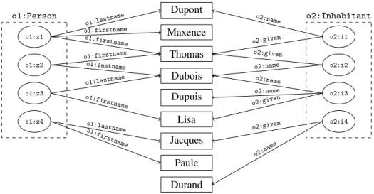
Example 1 (RDF dataset). Figure1 shows an example of two simple datasets (o1 and o2) to be interlinked. These datasets respectively represent instances of classes Person and Inhabitant. The first dataset describes persons using properties lastname and firstname. The second dataset makes use of properties name and given to describe inhabitants. All these properties are datatype properties. Hence, the signature of o1 is⟨{} {o1:lastname,o1:firstname} {o1:Person}⟩ and that of o2 is ⟨{} {o2:name,o2:given} {o2:Inhabitant}⟩.
Each dataset is populated with four instances. In the first dataset, there are instances z1, z2, z3, and z4. In the second dataset, instances are i1, i2, i3, and i4.
For example, the first dataset states that z1 is an instance of Person who has lastname "Dupont" and firstname "Thomas" and "Maxence". This example shows that properties can be multivalued: z1 has two firstnames and i3 two names. In this example, we assume that the following links have to be found: z1= i1, z2 = i2, and z3 = i3. Instances z4 and i4 are obviously different.
3.2. Link keys
Link keys specify the pairs of properties to compare for deciding whether individuals of two classes of two different datasets have to be linked. We first give the definition of a link key expression.
Definition 4 (Link key expression). A link key expression over two signatures⟨R,P,C⟩ and ⟨R′, P′,C′⟩ is an element of2(P×P′)∪(R×R′)×2(P×P′)∪(R×R′)×(C ×C′), i.e.
⟨{⟨pi, p′i⟩}i∈EQ,{⟨qj, q′j⟩}j∈IN,⟨c,c′⟩⟩ such that EQ and IN are (possibly empty) finite sets of indices.
In this section, we do not take into account the object property part of signatures which will be considered in Section6.
In order to make the notation more legible, sometimes we will write: {⟨pi, p′i⟩}i∈EQ{⟨qj, q′j⟩}j∈IN linkkey⟨c,c′⟩
The two sets of conditions are respectively called∀-conditions and ∃-conditions to distinguish them from the former EQ- and IN-conditions [4]: IN-conditions are the same as∃-conditions, but EQ-conditions correspond to both∀- and ∃-conditions.
Link key expressions may be compared and combined through subsumption, meet or join.
Definition 5 (Subsumption, meet and join of link key expressions). Let K= ⟨E,I,⟨c,c′⟩⟩ and H = ⟨F,J,⟨c,c′⟩⟩ be two link key expressions over the same pair of signatures⟨R,P,C⟩ and ⟨R′, P′,C′⟩. We say that K is subsumed by H, written K⊴ H, if E ⊆ F and I ⊆ J. Additionally, the meet and join of K and H, denoted by K △ H and K▽H, respectively, are defined as follows:
K△H =⟨E ∩F,I ∩J,⟨c,c′⟩⟩ K▽H =⟨E ∪F,I ∪J,⟨c,c′⟩⟩
For any finite set of link key expressions over the same pair of signatures, their meet and join are well-defined and each element of the set subsumes the meet and is subsumed by the join (K△H ⊴ K ⊴ K▽H).
Notation: we write K⊲ H when K ⊴ H and not H ⊴ K (H ⋬ K).
We only consider subsumption, meet and join of link key expressions over the same pair of classes and the same pair of signatures. When two link key expressions are defined over different pairs of signatures, the union of the signatures can be used to provide a common pair of signatures.
So far, link key expressions have been defined over signatures independently of actual datasets: they are only syntactic expressions. Intuitively, a link key expression⟨{⟨pi, p′i⟩}i∈EQ,{⟨qj, q′j⟩}j∈IN,⟨c,c′⟩⟩ generates a link, denoted by⟨o,o′⟩, between two individuals o and o′of c and c′, respectively, if o has the same values for p
ias o′ has for p′
i (for each i∈ EQ) and o and o′share at least one value for qjand q′j( j∈ IN). More formally:
Definition 6 (Link set generated by a link key expression). Let D and D′be two datasets of signatures⟨R,P,C⟩ and ⟨R′, P′,C′⟩, respectively. Let K = ⟨{⟨p
i, p′i⟩}i∈EQ,{⟨qj, q′j⟩}j∈IN,⟨c,c′⟩⟩ be a link key expression over their signature. Thelink set generated by K for D and D′is the subset LD,D
′ K ⊆ cD×c′D ′ defined as: ⟨o,o′⟩ ∈ LD,D′ K iff ⎧⎪⎪ ⎨⎪⎪ ⎩ pDi (o) = p′D ′
i (o′) for all i∈ EQ, and qDj(o)∩q′Dj ′(o′) ≠ ∅ for all j ∈ IN If no confusion arises, we may write LK instead of LD,D
′
K .
Example2illustrates the use of all the definitions introduced so far.
Example 2 (Link key expressions and link sets). Figure1shows an example of two simple datasets (o1 and o2) to be interlinked. From their signature, it is possible to define the following link key expressions:
K1= ⟨{}, {⟨o1:firstname,o2:given⟩}, ⟨o1:Person,o2:Inhabitant⟩⟩ K2= ⟨{}, {⟨o1:lastname,o2:name⟩}, ⟨o1:Person,o2:Inhabitant⟩⟩
K3= K1▽K2= ⟨{}, {⟨o1:firstname,o2:given⟩,⟨o1:lastname,o2:name⟩}, ⟨o1:Person,o2:Inhabitant⟩⟩ K4= ⟨{⟨o1:firstname,o2:given⟩,⟨o1:lastname,o2:name⟩}, {}, ⟨o1:Person,o2:Inhabitant⟩⟩ K5= ⟨{⟨o1:lastname,o2:given⟩}, {}, ⟨o1:Person,o2:Inhabitant⟩⟩
Such link key expressions would generate the following link sets: Lo1K,o2
1 = {⟨o1:z1,o2:i1⟩,⟨o1:z2,o2:i2⟩,⟨o1:z3,o2:i3⟩,⟨o1:z1,o2:i2⟩,⟨o1:z2,o2:i1⟩}
Lo1K,o2
2 = {⟨o1:z1,o2:i1⟩,⟨o1:z2,o2:i2⟩,⟨o1:z3,o2:i3⟩,⟨o1:z3,o2:i2⟩,⟨o1:z2,o2:i3⟩}
Lo1K,o2
3 = L
o1,o2
K1 ∩L
o1,o2
K2 = {⟨o1:z1,o2:i1⟩,⟨o1:z2,o2:i2⟩,⟨o1:z3,o2:i3⟩}
Lo1K,o2
4 = {⟨o1:z2,o2:i2⟩}
Lo1K,o2
The difference between∃-conditions and ∀-conditions is visible in the set of links generated by K3and K4. In the latter case, all property values should be in both instances for being linked; in the former, one common value is sufficient. The link key expression that would generate the expected links for Example1is K3.
With respect to link generation, subsumption, meet and join behave like set inclusion, intersection and union as the∀- and ∃-conditions are independent. The following lemma makes explicit the relations between these operations and the generated link sets.
Lemma 1. Let K, H, K1, . . . , Knbe link key expressions for two datasets D and D′over the same pair of classes. The following holds (omitting the mention of the two datasets):
If K⊴ H then LH⊆ LK (1) L△n k=1Kk⊇ n ⋃ k=1 LKk (2) L▽n k=1Kk= n ⋂ k=1 LKk (3)
Proof. In order to prove this lemma, we introduce the notion of the satisfaction of a link key condition. We say that a link⟨o,o′⟩ satisfies the ∀-conditions {⟨p
i, p′i⟩}i∈EQ in datasets D and D′if∀i ∈ EQ, pDi (o) = p′D
′
i (o
′) and that it satisfies the∃-conditions {⟨qj, q′j⟩}j∈IN in datasets D and D′if∀ j ∈ IN,qDj(o)∩q′D
′
j (o′) ≠ ∅. This is noted ⟨o,o′⟩ ∝ {⟨p
i, p′i⟩}i∈EQand⟨o,o′⟩ ∝ {⟨qj, q′j⟩}j∈IN(omitting the mention of the two datasets). (1) If K⊴ H, with K = ⟨E,I,⟨c,c′⟩⟩, it can be assumed that H = ⟨E ∪F,I ∪J,⟨c,c′⟩⟩. Hence, ∀l ∈ L
H, l∝ E ∪F and l∝ I ∪J, thus l ∝ E and l ∝ I which means that l ∈ LK. Therefore, LH⊆ LK.
(2) l∈ ⋃nk=1LKk⇔ ∃k ∈ 1..n;l ∈ LKk⇔ ∃k ∈ 1..n;l ∝ Ek∧l ∝ Ik⇒ l ∝ ⋂ n k=1Ek∧l ∝ ⋂nk=1Ik⇔ l ∈ L△nk=1Kk. Hence, ⋃n k=1LKk⊆ L△nk=1Kk. (3) l∈ ⋂nk=1LKk⇔ ∀k ∈ 1..n,l ∈ LKk⇔ ∀k ∈ 1..n,l ∝ Ek∧l ∝ Ik⇔ l ∝ ⋃ n k=1Ek∧l ∝ ⋃nk=1Ik⇔ l ∈ L▽n k=1Kk. Hence, ⋂n k=1LKk= L▽n k=1Kk.
Property1shows that if several link keys generate the same links, there is a link key that subsumes them and generates the same set of links.
Property 1. The join of a set of link key expressions generating the same set of links, generates that same set of links.
Proof. This is a direct consequence of Lemma1(3).
The capability of link key expressions to generate links across datasets, i.e. as link specifications, should now be clear. What is more difficult is to find the link key expression that generates the correct links. Of course, in principle, we do not know in advance which links are correct or not. We developed an algorithm which searches for link key candidates first before selecting the most promising candidate based on statistical evaluation [5]. Link key candidates are those link key expressions that, given a pair of datasets, would produce unique sets of links.
The definition of a link key candidate that we will use in this paper extends the one that we introduced in [5] by closing them by join. The link key candidates considered in [5] are now called “base link key candidates”. Such a base link key candidate is a link key expression that generates at least one link⟨o,o′⟩, and that is maximal among, i.e. subsumes, all the other link key expressions (over the same pair of classes) that also generate⟨o,o′⟩. The maximal link key expression is the only normal form identifying a unique set of generated links. It may cover many non maximal link key expressions generating the same links, several of which may be minimal.
Definition 7 (Base link key candidate). Let D and D′ be two datasets and K a link key expression over their signatures, K is abase link key candidate for D and D′if
A1. there exists l∈ LD,D
′
K , and
A2. if H is another link key expression over the same pair of classes as K such that l∈ LD,D
′
H and K⊴ H then K= H.
A link key candidate is defined as a link key expression that generates at least one link and that is maximal for all the other link key expressions that generate the same link set. The reasons to extend our previous definition [5] are that (a) it more directly shows the link with formal concept analysis, and (b) candidate link keys obtained by join, which were not caught by the previous definition, are sometimes the best candidates (as illustrated in the forthcoming Example4).
Definition 8 (Link key candidate). Let D and D′be two datasets and K a link key expression over their signatures, K is alink key candidate for D and D′if
B1. LD,D ′ K ≠ ∅, and B2. K= ▽H∈[K]H such that[K] = {H ∣ LD,D ′ K = L D,D′ H }
Intuitively, the set of link key expressions can be quotiented by the link sets they generate. This forms a partition of the link key expressions. Link key candidates are the maximal elements of the classes of this partition (Property1).
Lemma 2. Base link key candidates are link key candidates.
Proof. Given a link key candidate K, since l∈ LK, then LK≠ ∅. Moreover, if K is a base link key candidate, it is maximal for a particular link l∈ LK, i.e. there does not exist a link key expression H such that K⊲ H (and thus not generating other links than those of LK, because L is antimonotonic, Lemma1(1)) that generates this link. This means that K is maximal for LK. Hence, K is a link key candidate.
Lemma 3 (The set of link key candidates is closed by meet). The meet of every finite set of link key candidates is a link key candidate.
Proof. We need to prove that for any finite set{Ki}i∈I of link key candidates, △i∈IKi is a link key candidate. If for some j∈ I; Kj= △i∈IKi, then this is true. Considering that this is not the case, then necessarily, ∀ j ∈ I, LKj ≠ L△i∈IKi, otherwise, Kj would not be a link key candidate (not maximal). If △i∈IKi were not a link key
candidate, this would mean that there exists H such that L△i∈IKi = L(△i∈IKi)▽H and H⋬ △i∈IKi. This entails that ∃ j ∈ I, such that l ∈ LKj and l/∈ LKj▽H, hence l/∈ LH (by Lemma1(3)). Hence, l∈ L△i∈IKi (by Lemma1(2)) and
l/∈ L
△i∈IKi▽H(by Lemma1(3)), thus L△i∈IKi≠ L(△i∈IKi)▽H which contradicts the hypothesis.
The following proposition proves that being a link key candidate is equivalent to being a base link key candi-date or the meet of base link key candicandi-dates.
Proposition 2. The set of link key candidates is the smallest set containing all the base link key candidates that is closed by meet.
Proof. (1) The set of link key candidates contains all base link key candidates (Lemma2). (2) The set of link key candidates is closed by meet (Lemma3).
(3) The set of link key candidates is the smallest such set. If this were not the case, there would exist a link key candidate K not base and not obtained through the meet of link key candidates. There are two cases:
– either K is directly subsumed by the maximal link key candidate. Then, K generates at least one more link than the maximal link key candidate (otherwise it would not be a link key candidate because it would not be maximal for the link set it generates) and so K is a base link key candidate which contradicts the hypothesis. – or there exists a set of link key candidates{Ki}i∈Isubsuming K. This means that K is also subsumed by their
meet (∀i ∈ I, K ⊲ Kientails K⊴ △i∈IKi). Since, K≠ △i∈IKiby hypothesis, then K⊲ △i∈IKiand thus L△i∈IKi⊂ LK
(by Lemma 1(1) and because K would not be maximal if it would generate the same link set). Thus, there exists l∈ LK∖ L△i∈IKi and K is maximal for l (apparently no link key candidate that subsumes K generates l),
hence K is a base link key candidate and this contradicts the hypothesis.
Intuitively, this means that link key candidates are either base link key candidates or the meet of base link key candidates which is not maximal for any particular link (because for any link l∈ L△i∈IKi, there exist i such as
l∈ LKi) but nonetheless generates a distinct set of links. Hence from the base link key candidates we can generate
the set of link key candidates. However, we will show how to generate them directly with formal concept analysis.
4. A short introduction to FCA and RCA
We briefly introduce the principles of formal concept analysis and relational concept analysis which will be used to extract link key candidates.
4.1. Basics of formal concept analysis
Formal Concept Analysis (FCA) [23] starts with a binary context⟨G,M,I⟩ where G denotes a set of objects, M a set of attributes, and I⊆ G×M a binary relation between G and M, called the incidence relation. The statement gImis interpreted as “object g has attribute m”. Two operators⋅↑and⋅↓ define a Galois connection between the powersets⟨2G,⊆⟩ and ⟨2M,⊆⟩, with A ⊆ G and B ⊆ M:
A↑= {m ∈ M ∣ gIm for all g ∈ A} B↓= {g ∈ G ∣ gIm for all m ∈ B} The operators⋅↑and⋅↓are decreasing, i.e. if A
1⊆ A2then A↑2⊆ A↑1and if B1⊆ B2then B↓2⊆ B↓1. Intuitively, the less objects there are, the more attributes they share, and dually, the less attributes there are, the more objects have these attributes. Moreover, it can be checked that A⊆ A↑↓and that B⊆ B↓↑, that A↑= A↑↓↑and that B↓= B↓↑↓.
For A⊆ G, B ⊆ M, a pair ⟨A,B⟩, such that A↑= B and B↓= A, is called a formal concept, where A is the extent and B the intent of⟨A,B⟩. Moreover, for a formal concept ⟨A,B⟩, A and B are closed sets for the closure operators ⋅↑↓and⋅↓↑, respectively, i.e. A↑↓= A and B↓↑= B.
Concepts are partially ordered by⟨A1, B1⟩ ≤ ⟨A2, B2⟩ ⇔ A1⊆ A2or equivalently B2⊆ B1. With respect to this partial order, the set of all formal concepts forms a complete lattice called the concept lattice of⟨G,M,I⟩.
Datasets are often complex with attribute values not ranging in Booleans, e.g. numbers, intervals, strings. Such data can be represented as a many-valued context⟨G,M,W,I⟩, where G is a set of objects, M a set of attributes, W a set of values, and I a ternary relation defined on the Cartesian product G×M ×W. The fact ⟨g,m,w⟩ ∈ I or simply m(g) = w means that object g takes the value w for the attribute m. In addition, when ⟨g,m,w⟩ ∈ I and ⟨g,m,v⟩ ∈ I then w= v [23]: in FCA, “many-valued” means that the range of an attribute may include more than two values, but for any object, the attribute can only have one of these values.
Conceptual scaling can be used for transforming a many-valued context into a one-valued context. For exam-ple, if Wm= {w1, w2, . . . wp} ⊆ W denotes the range of the attribute m, then a scale of elements “m = wi,∀wi∈ Wm” is used for binarising the initial many-valued context. Intuitively, a scale splits the range Wmof a valued attribute minto a set of p binary attributes “m= wi, i= 1,..., p”. There are many possible scalings and some of them are detailed in [23]. Another specific example of scaling is proposed hereafter for building relational attributes.
Conceptual scaling generally produces larger contexts than the original contexts —as the number of attributes increases. However, it is also possible to avoid scaling and to directly work on complex data, using the formalism of “pattern structures” [22,28].
4.2. Relational concept analysis
Relational Concept Analysis (RCA) [40] extends FCA to the processing of relational datasets and allows inter-object relations to be materialised and incorporated into formal concept intents.
RCA is defined by a relational context family, composed of a set of formal contexts{⟨Gx, Mx, Ix⟩}x∈Xand a set of binary relations{ry}y∈Y. A relation ry⊆ Gx× Gz connects two object sets, a domain Gx(dom(ry) = Gx, x∈ X) and a range Gz(ran(ry) = Gz, z∈ X). The expression ry(g) denotes the set of objects in Gzrelated to g through ry. RCA is based on a relational scaling mechanism that transforms a relation ryinto a set of relational attributes that are added to the context describing the object set dom(ry), as made precise below. Various relational scaling operators exist in RCA such as existential, strict and wide universal, min and max cardinality, which all follow the classical role restriction semantics in description logics [8]. For example, strict universal scaling, consists of adding the attribute∃∀ry.C to Mxand to have gI∃∀ry.C whenever ry(g) ≠ ∅ and ry(g) ⊆ extent(C), i.e. whenever there exists an object related to g by ryand all such objects belong to the extent of concept C.
Practically, in the case of strict universal scaling for example, let us consider two sets of objects, say Gxand Gz, their associated concept lattices Lxand Lz, and a relation ry⊆ Gx× Gz. For each C∈ Lzfor which there exists a pair of objects gx∈ Gxand gz∈ extent(C) such that ry(gx, gz) and for all gz∈ ry(gx), gz∈ extent(C), the process adds a new relational attribute∃∀ry.C to Mx.
The base RCA algorithm proceeds in the following way:
1. Initial formal contexts are for each x∈ X, ⟨Gx, Mx0, Ix0⟩ = ⟨Gx, Mx, Ix⟩.
2. For each formal context⟨Gx, Mtx, Itx⟩ the corresponding concept lattice Ltxis created using FCA.
3. Relational scaling is applied, for each relation rywhose codomain lattice has new concepts, generating new contexts⟨Gx, Mt+1x , Ixt+1⟩ including both plain and relational attributes in Mt+1x .
4. If scaling has occurred (∃x ∈ X;Mxt+1≠ Mxt), go to Step2. 5. The results is a set of lattices{Ltx}x∈X.
5. Formal contexts for independent link key candidates
In [6], the link key candidate extraction problem for databases was encoded in FCA. In this case, the set of database link key candidates exactly corresponds to the concepts of a one-valued context [23]. A concept⟨L,K⟩ resulting from this encoding has as intent K a link key candidate and as extent L the link set it generates.
We generalise our encoding to the case of non functional datasets, such as RDF datasets, by adapting the link key conditions presented in Definition4. These conditions deal with value multiplicity. The encoding of both conditions goes as follows, for each pair of properties⟨p, p′⟩ ∈ P × P′, two attributes can be generated: ∃⟨p, p′⟩ and∀⟨p, p′⟩ referred to, as before, as ∃-condition or ∀-condition.
Definition 9 (Formal context for independent link key candidates). Given two datasets D of signature⟨R,P,C⟩ and D′of signature⟨R′, P′,C′⟩, the formal context for independent link key candidates between a pair of classes ⟨c,c′⟩ of C ×C′is⟨cD×c′D′,{∃,∀}×P×P′, I⟩ such that:
⟨o,o′⟩ I ∀⟨p, p′⟩ iff pD(o) = p′D′(o′) (∀)
⟨o,o′⟩ I ∃⟨p, p′⟩ iff pD(o)∩ p′D′
(o′) ≠ ∅ (∃)
We introduce the∀∃ notation corresponding to:
⟨o,o′⟩ I ∀∃⟨p, p′⟩ iff pD(o) = p′D′(o′) ≠ ∅ (∀∃)
which exactly corresponds to satisfying both∀- and ∃-conditions, i.e. the values of the properties must be the same and there should be at least one such value. So they are only used as a shortcut when both (∀) and (∃) hold. The Galois connection associated with such a formal context for link key candidates can be made explicit, as introduced in Section4. Given two datasets D of signature⟨R,P,C⟩ and D′of signature⟨R′, P′,C′⟩ and a pair of classes⟨c,c′⟩ ∈ C ×C′, a Galois connection between the power sets 2(cD×c′D
′ ) and 2({∃,∀}×P×P′)is defined as follows: .↑∶ 2(cD×c′D ′ )Ð→ 2({∃,∀}×P×P′)
L↑= {∃⟨p, p′⟩∣ for all ⟨o,o′⟩ ∈ L,⟨o,o′⟩ I ∃⟨p, p′⟩}∪{∀⟨p, p′⟩∣ for all ⟨o,o′⟩ ∈ L,⟨o,o′⟩ I ∀⟨p, p′⟩}
.↓∶ 2({∃,∀}×P×P′
)Ð→ 2(cD×c′D
′
)
K↓= {⟨o,o′⟩∣ for all ∃⟨p, p′⟩ ∈ K,⟨o,o′⟩ I ∃⟨p, p′⟩ and for all ∀⟨p, p′⟩ ∈ K,⟨o,o′⟩ I ∀⟨p, p′⟩} It should be clear from the definitions that for any pair of datasets D and D′, K↓= LD,D
′
K .
Example3minimally illustrates the discovery of relevant link key candidates in FCA, but Example4is more elaborate.
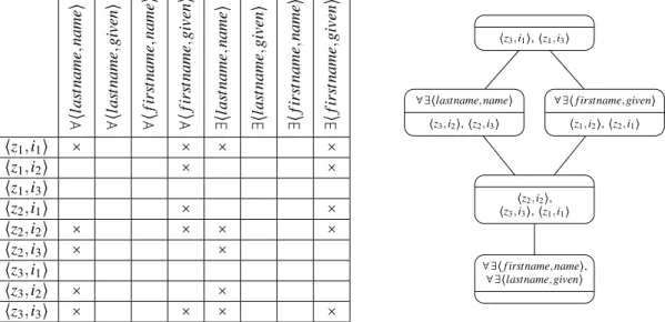
Example 3 (Simple independent link key candidate extraction). Let us consider the two simple datasets given in Figure2. We assume that classeso1:Personando2:Inhabitantoverlap, so we expect to find some link key candidates between these two classes. Following Definition9, the formal context encoding the link key candidate extraction problem is built. This formal context is given in the table of Figure3(left), where instances z2 and i3 share at least one value, e.g. "Dubois", for the pair of properties lastname and name. In this simple example, since all properties are functional,∀ and ∃ quantifications have identical columns. So, in the resulting lattice all the intent conditions are prefixed by∀∃. This leads to the concept lattice given in Figure3 featuring five concepts. The concept ⟨{⟨z1, i1⟩,⟨z2, i2⟩,⟨z3, i3⟩},{∀∃ ⟨lastname,name⟩,∀∃ ⟨firstname,given⟩}⟩ whose in-tent represents the link key candidate{∀∃ ⟨lastname,name⟩,∀∃ ⟨firstname,given⟩} would generate the links {⟨z1, i1⟩,⟨z2, i2⟩,⟨z3, i3⟩} (its extent) if used as a link key. This candidate is a perfect link key since it would gen-erate all and only expected links. Other candidates that only use “lastname” or “firstname” would also gengen-erate all links but also wrong links since different persons may share either firstname or lastname.
This encoding correctly conveys the notion of link key candidates as shown by the following proposition. Proposition 3. K is a link key candidate for datasets D and D′if and only if⟨K↓, K⟩ is a formal concept of the formal context for link key candidates in D and D′and K↓≠ ∅.
In other terms, this means that⟨{⟨pi, p′i⟩}i∈EQ,{⟨qj, q′j⟩}j∈IN,⟨c,c′⟩⟩ is a link key candidate for datasets D and D′if and only if K= {∀⟨p
i, p′i⟩}i∈EQ∪ {∃⟨qj, q′j⟩}j∈IN is the intent of a concept generated by the formal context for link key candidates between c and c′and K↓≠ ∅.
o1:Person o1:z1 o1:z2 o1:z3 o2:Inhabitant o2:i1 o2:i2 o2:i3 Dupont Thomas Dubois Lisa o1:lastname o1:lastname o1:lastname o1:firstname o1:firstname o1:firstname o2:given o2:given o2:given o2:name o2:name o2:name
Figure 2: Example of two datasets representing respectively instances of classes Person and Inhabitant.
∀ ⟨l as tname ,name ⟩ ∀ ⟨l as tname ,given ⟩ ∀ ⟨ fir st name ,name ⟩ ∀ ⟨ fir st name ,given ⟩ ∃⟨ las tname ,name ⟩ ∃⟨ las tname ,given ⟩ ∃⟨ fir st name ,name ⟩ ∃⟨ fir st name ,given ⟩ ⟨z1, i1⟩ × × × × ⟨z1, i2⟩ × × ⟨z1, i3⟩ ⟨z2, i1⟩ × × ⟨z2, i2⟩ × × × × ⟨z2, i3⟩ × × ⟨z3, i1⟩ ⟨z3, i2⟩ × × ⟨z3, i3⟩ × × × × ∀∃⟨lastname, name⟩ ⟨z3, i2⟩, ⟨z2, i3⟩ ∀∃⟨f irstname, name⟩, ∀∃⟨lastname, given⟩ ⟨z3, i1⟩, ⟨z1, i3⟩ ⟨z2, i2⟩, ⟨z3, i3⟩, ⟨z1, i1⟩ ∀∃⟨f irstname, given⟩ ⟨z1, i2⟩, ⟨z2, i1⟩
Figure 3: Formal context (left) and corresponding concept lattice (right) for the classeso1:Personando2:Inhabitantof Figure2.
Proof. The proof of the property is as follows. In both cases, K↓= L
K≠ ∅ (and we leave the D and D′implicit). From Definition8, K is a link key candidate if LK≠ ∅ and K = ▽H∈[K]Hsuch that[K] = {H ∣ L
D,D′
K = L
D,D′
H }.
(⇒) Hence K is maximal for LK= K↓(Property1), which means that K↓↑= K, thus ⟨LK, K⟩ is a concept. (⇐) Conversely, if ⟨K↓, K⟩ is a concept, K↓= L
K and K is the maximal link key expression generating LK, hence it is a link key candidate.
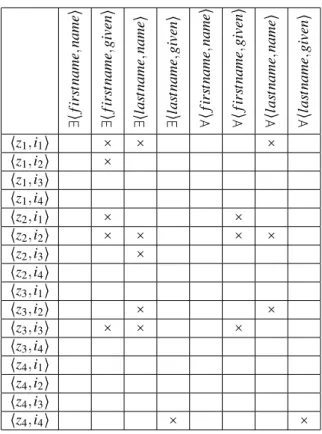
Example 4 (Extraction of independent link key candidates over more complex data, as presented in Example1). The datasets presented in Example3were very simple. Let us consider the dataset presented in Figure1. The interlinking problem is now encoded in the context given in Table 1 and the resulting lattice is presented in Figure 4. The concepts corresponding to link key expressions of Example 2 are labelled by a +. Since some properties are multivalued, the lattice now contains some candidates with the same sets of properties but with different quantifications. For instance, there are two candidates whose intents are{∃⟨firstname,given⟩} and {∀∃ ⟨firstname,given⟩}. The former is less restrictive and then it would generate all the links generated by the latter plus the link⟨z1, i2⟩ (because p1has the two firstnames "Maxence" and "Thomas" and i2has only "Thomas"). In this example, the perfect link key is labelled⋆ whose intent is {∃⟨firstname,given⟩,∃⟨lastname,name⟩}. This is a link key candidate, butnot a base link key candidate: it does not generate any link which is not generated by its subsumees.
6. Hierarchically dependent link key candidates
So far, the proposed approach only dealt with datatype properties, i.e. properties whose value is not another object [16]. However, it may happen that the ranges of properties are themselves objects. These are called object properties or simply relations.
Determining if values of such properties across two datasets are equal or intersect requires to be able to identify them. This is exactly the role of link keys. Hence, link key candidates for pair of classes having object properties should rely on the link key candidates attached to the range of such properties.
∃⟨ fir st name ,name ⟩ ∃⟨ fir st name ,given ⟩ ∃⟨ las tname ,name ⟩ ∃⟨ las tname ,given ⟩ ∀ ⟨ fir st name ,name ⟩ ∀ ⟨ fir st name ,given ⟩ ∀ ⟨l as tname ,name ⟩ ∀ ⟨l as tname ,given ⟩ ⟨z1, i1⟩ × × × ⟨z1, i2⟩ × ⟨z1, i3⟩ ⟨z1, i4⟩ ⟨z2, i1⟩ × × ⟨z2, i2⟩ × × × × ⟨z2, i3⟩ × ⟨z2, i4⟩ ⟨z3, i1⟩ ⟨z3, i2⟩ × × ⟨z3, i3⟩ × × × ⟨z3, i4⟩ ⟨z4, i1⟩ ⟨z4, i2⟩ ⟨z4, i3⟩ ⟨z4, i4⟩ × ×
Table 1: Formal context for the classeso1:Personando2:Inhabitantof Figure1.
Precisely, dealing with pairs of object properties⟨r,r′⟩ whose range is the pair of classes ⟨d,d′⟩ requires to know how to compare the members of d and d′in order to decide if rD(o) = r′D′(o′) or if rD(o) ∩ r′D′(o′) ≠ ∅. Comparison of sets of values in the definition of link sets generated by a link key candidate (Definition6) and in the definition of the incidence relation (Definition9) is achieved by using link key expressions on the range classes (Definition10).
Definition 10 (Comparison of sets of instances). Given two sets S and S′of instances of classes d and d′and K a link key expression for the pair⟨d,d′⟩, =
Kand∩K are defined by:
S=KS′ iff ∀x ∈ S,∃x′∈ S′;⟨x,x′⟩ ∈ K↓and∀x′∈ S′,∃x ∈ S;⟨x,x′⟩ ∈ K↓ S∩KS′≠ ∅ iff K↓∩(S ×S′) ≠ ∅
The use of these comparisons is only well-defined when there is no cyclic dependency across link key expres-sions.
This can be used in order to extend the formal contexts to dependent link key candidates:
Definition 11 (Formal context for dependent link key candidates). Given two datasets D of signature⟨R,P,C⟩ and D′of signature⟨R′, P′,C′⟩, for any pair of object properties ⟨r,r′⟩ ∈ R × R′, letK
r,r′ the set of dependent link key
candidates associated with the range of r and r′. Theformal context for dependent link key candidates between a pair of classes⟨c,c′⟩ of C ×C′is⟨cD×c′D′,{∀,∃}×((P×P′)∪{⟨r,r′, K⟩;r ∈ R,r′∈ R′, K∈ K
r,r′}),I⟩ such that:
⟨o,o′⟩ I ∀⟨p, p′⟩ iff pD(o) = p′D′(o′) ⟨o,o′⟩ I ∃⟨p, p′⟩ iff pD(o)∩ p′D′
(o′) ≠ ∅ ⟨o,o′⟩ I ∀⟨r,r′⟩ K iff rD(o) =Kr′D ′ (o′) ⟨o,o′⟩ I ∃⟨r,r′⟩ K iff rD(o)∩Kr′D ′ (o′) ≠ ∅
In principle, a link key is the way to identify the instances of a pair of classes. Hence, comparing the values of two properties should be done with the link key extracted for the classes of these values. For this reason, link key expressions (Definition4) do not refer to the link keys to use as Definition11. This means that the extracted
∀∃⟨lastname, given⟩ ⟨z4, i4⟩ ⟨z4, i3⟩, ⟨z2, i4⟩, ⟨z1, i3⟩, ⟨z3, i4⟩, ⟨z1, i4⟩, ⟨z4, i1⟩, ⟨z4, i2⟩, ⟨z3, i1⟩ ∀∃⟨f irstname, name⟩ ∀∃⟨f irstname, given⟩ ⟨z2, i1⟩ ⟨z2, i2⟩ ∀∃⟨lastname, name⟩ ⟨z3, i2⟩ ∃⟨lastname, name⟩ ⟨z2, i3⟩ ∃⟨f irstname, given⟩ ⟨z1, i2⟩ ⟨z3, i3⟩ ⟨z1, i1⟩ + + + + + ⋆
Figure 4: Concept lattice built from the context of Table1for the classeso1:Personando2:Inhabitant.
link keys should only rely on each others. We aim at extracting such sets of link key candidates. We call them coherent families of link key candidates.
For simplifying the presentation we introduce the notion of alignment. An alignment in general is made of a set of relations between ontology entities [19]. For the purpose of this paper, it will simply be a set of pairs of classes considered as overlapping. A coherent set of link key candidates with respect to an alignment is called a coherent family of link key candidates.
Definition 12 (Coherent family of link key candidates). Given two datasets D of signature⟨R,P,C⟩ and D′of signature⟨R′, P′,C′⟩, and an alignment A ⊆ C ×C′between their classes, acoherent family of link key candidates for D and D′related by A is a collection of dependent link key candidates:
T= {K⟨c,c′⟩}⟨c,c′⟩∈A
such that each link key in T only depends on other link keys in T (compatibility).
Any collection of independent link key candidates with respect to an alignment A is a coherent family of link key candidates.
The key dependency graph of a coherent family of link key candidates is the directed graph whose vertices are the link key candidates and there is an edge from one link key candidate to another if the former depends on the latter. A coherent family of link key candidates is said to be “acyclic” if its key dependency graph contains no cycle, including unit cycle. Otherwise, it is called “cyclic”.
When classes are hierarchically organised, coherent families of link key candidates are necessarily acyclic. They can be obtained inductively through the following algorithm:
1. Generate the (independent) link key candidates for pairs of classes having no object properties, using the formal contexts of Definition9.
2. For each pair of classes that only depends on pairs of classes having been processed, build formal contexts according to Definition11.
3. If there are still pairs of classes in A to process, go to Step2.
4. Extract the coherent families by picking one link key candidate per pair of classes in A, as long as they are compatible.
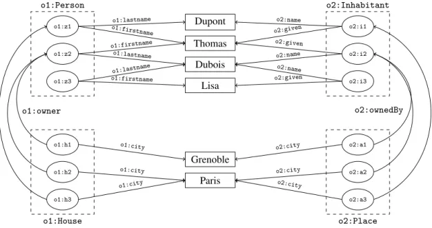
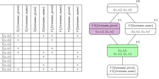
Example 5 (Acyclic link key candidate extraction). Figure5, shows two datasets that both describe instances from classes House, resp. Place, that are in relation with instances from classes Person, resp. Inhabitant. First, the formal context between the two independent classes Person and Inhabitant is used to build the corresponding lattice, see Figure6. Four link key candidates, named C0, C1, C2, C3, are extracted.
From these candidates, it can be dealt with classes which only depend on the aligned pairs handled in the former steps, e.g. the pair of classes Person and Inhabitant. The formal context for these two classes is given in Figure7. Contrasting datatype properties, the pair⟨owner,ownedBy⟩ (whose domains are classes House and Place) is taken into account according to the four link key candidates generated for classes Person and Inhabitant. The resulting lattice is given in Figure7using a reduced notation, i.e. when the intent of a concept contains several concepts computed at previous steps, only the most specific ones are kept. For example, concept D3 could also include∀∃ ⟨owner,ownedBy⟩C0in its intent, but since C1 is more constraining than C0, then only ∀∃ ⟨owner,ownedBy⟩C1is retained.
In the two lattices, compatible concepts are coloured: purple for C1−D1 and C1−D3, and green for C2−D0 and C2− D2. The green colour is reserved to the link key candidates that were expected; dotted pattern is used for candidates that are not part of any coherent family of link key candidates. The lattice shows that the intent of concept D0, i.e. {∀∃ ⟨owner,ownedBy⟩C2,∀∃ ⟨city,city⟩}, is the best link key candidate since it generates all and only expected links.
o1:Person o1:z1 o1:z2 o1:z3 o1:House o1:h1 o1:h2 o1:h3 o2:Inhabitant o2:i1 o2:i2 o2:i3 o2:Place o2:a1 o2:a2 o2:a3 Dupont Thomas Dubois Lisa Grenoble Paris o1:lastname o1:lastname o1:lastname o1:firstname o1:firstname o1:firstname o2:given o2:given o2:given o2:name o2:name o2:name o1:owner o2:ownedBy o1:city o1:city o1:city o2:city o2:city o2:city
Figure 5: Two datasets representing instances of class House (resp. Place) that are in relation through the owner property, (resp. ownedBy) with instances of class Person (resp. Inhabitants).
.
A limitation of this method is that it cannot handle cases in which the data dependencies involve cycles. We now consider this case.
7. Dealing with cyclic dependencies through relational concept analysis
Classes are not always hierarchically organised. Object properties may loop through the set of classes. Even if this does not affect resulting link key candidates, this cannot be ruled out.
To solve this problem we took inspiration from RCA [40]. Accordingly, the problem is modelled, as in RCA, through the set of formal contexts corresponding to pairs of classes and a set of relational contexts corresponding to pairs of object properties. We thus diverge from the solutions provided in Section6by initially recording only datatype properties within the formal contexts (Definition9) and using relational contexts for object properties.
The main difference with RCA is that RCA is designed for extracting conceptual descriptions of classes, though we aim at extracting link key candidates. The former describes classes, the latter describes how to identify instances. Another difference is that coherent families of link key candidates have no analogous notion in RCA as all class descriptions may coexist: no compatibility is requested. However, at the technical level of concept
∃⟨ fir st name ,given ⟩ ∃⟨ fir st name ,name ⟩ ∃⟨ las tname ,given ⟩ ∃⟨ las tname ,name ⟩ ∀ ⟨f ir st name ,given ⟩ ∀ ⟨f ir st name ,name ⟩ ∀ ⟨l as tname ,given ⟩ ∀ ⟨l as tname ,name ⟩ ⟨z1, i1⟩ × × × × ⟨z1, i2⟩ × × ⟨z1, i3⟩ ⟨z2, i1⟩ × × ⟨z2, i2⟩ × × × × ⟨z2, i3⟩ × × ⟨z3, i1⟩ ⟨z3, i2⟩ × × ⟨z3, i3⟩ × × × × ∀∃⟨lastname, name⟩ ⟨z3, i2⟩, ⟨z2, i3⟩ ∀∃⟨lastname, given⟩, ∀∃⟨f irstname, name⟩ ∀∃⟨f irstname, given⟩ ⟨z2, i1⟩, ⟨z1, i2⟩ ⟨z3, i1⟩, ⟨z1, i3⟩ ⟨z2, i2⟩, ⟨z3, i3⟩, ⟨z1, i1⟩ C0 C1 C2 C3
Figure 6: Formal context and concept lattice for Person and Inhabitant of Figure5.
. ∃⟨ ci ty ,ci ty ⟩ ∀ ⟨ci ty ,ci ty ⟩ ∃⟨ owner ,owned By ⟩C0 ∀ ⟨owner ,owned By ⟩C0 ∃⟨ owner ,owned By ⟩C1 ∀ ⟨owner ,owned By ⟩C1 ∃⟨ owner ,owned By ⟩C2 ∀ ⟨owner ,owned By ⟩C2 ∃⟨ owner ,owned By ⟩C3 ∀ ⟨owner ,owned By ⟩C3 ⟨h1, a1⟩ × × × × × × × × × × ⟨h1, a2⟩ × × × × × × × × ⟨h1, a3⟩ × × × × ⟨h2, a1⟩ × × × × × × × × ⟨h2, a2⟩ × × × × × × × × × × ⟨h2, a3⟩ × × × × × × ⟨h3, a1⟩ × × × × ⟨h3, a2⟩ × × × × × × ⟨h3, a3⟩ × × × × × × × × × × ∀∃⟨owner, ownedBy⟩C2 ⟨h2, a1⟩, ⟨h1, a2⟩ ∀∃⟨owner, ownedBy⟩C1 ⟨h3, a1⟩, ⟨h1, a3⟩ ⟨h1, a1⟩, ⟨h3, a3⟩, ⟨h2, a2⟩ ∀∃⟨city, city⟩ ⟨h2, a3⟩, ⟨h3, a2⟩ D0 D1 D2 D3
Figure 7: Dependent formal context and concept lattice for House and Place of Figure5.
discovery, the process is the same. In particular, the relational contexts are exactly the same. They are simply extended to pairs of properties and thus pairs of instances.
Definition 13 (Relational contexts for dependent link key candidates). Given two datasets D of signature⟨R,P,C⟩ and D′of signature⟨R′, P′,C′⟩ and an alignment A ⊆ C ×C′, given two pairs of classes⟨c,c′⟩ and ⟨d,d′⟩ of A and a pair of object properties⟨r,r′⟩ of R×R′, the relational context associated with r and r′in D and D′is defined by ⟨cD×c′D′
, dD×d′D′, I⟩ such that:
⟨x,x′⟩ I ⟨y,y′⟩ iff y ∈ rD(x) and y′∈ r′D′(x′)
Scaling operators are used for transferring the constraints from the relational contexts to the formal contexts. Definition 14 (Link key condition scaling operators). Given two datasets D of signature⟨R,P,C⟩ and D′of sig-nature⟨R′, P′,C′⟩, and a relational context ⟨cD×c′D′, dD×d′D′, I⟩ for a pair of object properties ⟨r,r′⟩ ∈ R×R′,
– the universal scaling operator f∀
r,r′∶ (cD×c′D ′ )×Kr,r′→ B is defined by f∀ r,r′(⟨o,o ′⟩,K) iff rD(o) = Kr′D ′ (o′), – the existential scaling operator f∃
r,r′∶ (c D×c′D′ )×Kr,r′→ B is defined by f∃ r,r′(⟨o,o ′⟩,K) iff rD(o)∩ Kr′D ′ (o′) ≠ ∅.
The universal and existential scaling operators scale the formal contexts in Definition9upon the∀-conditions and∃-conditions on the object property pairs of the relational contexts in Definition13.
Hence, a relational context family [40] can be associated to two datasets and an alignment:
Definition 15 (Relational context family for dependent link key candidates). Given two datasets D of signature ⟨R,P,C⟩ and D′of signature⟨R′, P′,C′⟩, and an alignment A ⊆ C ×C′, the relational context family for dependent link key candidate extraction between D and D′through A is composed of:
– all the formal contexts corresponding to pairs of classes in A,
– all the relational contexts corresponding to object property pairs in R×R′relating pairs of classes from A. The solution to the problem is a collection of concept lattices, one per pair of aligned classes in A, from which the coherent families of link key candidates may be extracted exactly like in Section6. The algorithm is that of relational concept analysis, using the link key condition scaling operators (Definition14):
1. Start with the formal contexts corresponding to aligned classes. 2. Apply formal concept analysis to all contexts.
3. Apply the scaling operators on the relational contexts to add columns in the formal contexts depending on the already extracted keys.
4. If scaling has occurred, go to Step2.
5. Extract the coherent families by picking one link key candidate per pair of classes in A, as long as they are compatible.
Example6illustrates the extraction of cyclic link key candidates.
Example 6 (Cyclic link key candidate extraction). Figure8provides an example of two datasets containing cir-cular dependencies. In the first, left-hand side, dataset, classes Person and House mutually depend on each other through relations home and owner. Respectively, in the second, right-hand side, dataset, classes Inhabitant and Place also mutually depend on each other through relations address and ownedBy. The relational context family is made of formal contexts presented in Figure9and relational contexts given in Figure10. It is iteratively scaled using the scaling operators of Definition14. It converges to a fix-point after six iterations. The final lattices are given in Figure11. We obtain two pairs of compatible concepts, namely C1−C2 and C4 −C6. The coherent family of link key candidates C4−C6 generates all and only relevant links.
8. Implementation and complexity considerations
One benefit of reformulating the link key candidate extraction problem as formal and relational concept analy-sis is to use directly standard algorithms for such problems. We implemented the proposed approach as a proof-of-concept in Python 33. The implementation took inspiration from another formal concept analysis implementation [39]. It uses the Norris algorithm [37] for performing FCA extended to deal with pairs of objects in the extent and quantified and qualified pairs of properties in the intent. The RCA processing has been implemented by iteratively
o1:Person o1:z1 o1:z2 o1:z3 o1:House o1:h1 o1:h2 o1:h3 o2:Inhabitant o2:i1 o2:i2 o2:i3 o2:Place o2:a1 o2:a2 o2:a3 Dupont Thomas Dubois Lisa Grenoble Paris o1:lastname o1:lastname o1:lastname o2:given o2:given o2:given o2:name o2:name o2:name o1:home
o1:owner o2:address o2:ownedBy
o1:city o1:city o1:city o2:city o2:city o2:city
Figure 8: Datasets illustrating mutual dependencies between classes.
∃⟨ las tname ,given ⟩ ∃⟨ las tname ,name ⟩ ∀ ⟨l as tname ,given ⟩ ∀ ⟨l as tname ,name ⟩ ⟨z1, i1⟩ × × ⟨z1, i2⟩ ⟨z1, i3⟩ ⟨z2, i1⟩ ⟨z2, i2⟩ × × ⟨z2, i3⟩ × × ⟨z3, i1⟩ ⟨z3, i2⟩ × × ⟨z3, i3⟩ × × ∃⟨ ci ty ,ci ty ⟩ ∀ ⟨ci ty ,ci ty ⟩ ⟨h1, a1⟩ × × ⟨h1, a2⟩ ⟨h1, a3⟩ ⟨h2, a1⟩ ⟨h2, a2⟩ × × ⟨h2, a3⟩ × × ⟨h3, a1⟩ ⟨h3, a2⟩ × × ⟨h3, a3⟩ × ×
Figure 9: Formal contexts for the pairs of classes⟨Person,Inhabitant⟩ and ⟨HousePlace⟩ in Figure8.
Rowner ,owned By ⟨z3 ,i1 ⟩ ⟨z3 ,i2 ⟩ ⟨z3 ,i3 ⟩ ⟨z2 ,i1 ⟩ ⟨z2 ,i2 ⟩ ⟨z2 ,i3 ⟩ ⟨z1 ,i1 ⟩ ⟨z1 ,i2 ⟩ ⟨z1 ,i3 ⟩ ⟨h1, a1⟩ × ⟨h1, a2⟩ × ⟨h1, a3⟩ × ⟨h2, a1⟩ × ⟨h2, a2⟩ × ⟨h2, a3⟩ × ⟨h3, a1⟩ × ⟨h3, a2⟩ × ⟨h3, a3⟩ × Rhome ,ad d ress ⟨h3 ,a2 ⟩ ⟨h3 ,a3 ⟩ ⟨h3 ,a1 ⟩ ⟨h2 ,a2 ⟩ ⟨h2 ,a3 ⟩ ⟨h2 ,a1 ⟩ ⟨h1 ,a2 ⟩ ⟨h1 ,a3 ⟩ ⟨h1 ,a1 ⟩ ⟨z1, i1⟩ × ⟨z1, i2⟩ × ⟨z1, i3⟩ × ⟨z2, i1⟩ × ⟨z2, i2⟩ × ⟨z2, i3⟩ × ⟨z3, i1⟩ × ⟨z3, i2⟩ × ⟨z3, i3⟩ ×
∀∃⟨lastname, given⟩ ∀∃⟨home, address⟩C8 ⟨z1, i3⟩, ⟨z3, i1⟩ ∀∃⟨home, address⟩C0, ∀∃⟨lastname, name⟩ ⟨z3, i2⟩, ⟨z2, i3⟩ ∀∃⟨home, address⟩C1 ∀∃⟨home, address⟩C5 ⟨z1, i2⟩, ⟨z2, i1⟩ ∀∃⟨home, address⟩C4 ⟨z2, i2⟩, ⟨z1, i1⟩, ⟨z3, i3⟩ C2 C3 C6 C7 C9 ∀∃⟨owner, ownedBy⟩C7 ⟨h3, a1⟩, ⟨h1, a3⟩ ∀∃⟨owner, ownedBy⟩C2 ∀∃⟨owner, ownedBy⟩C9, ∀∃⟨city, city⟩ ⟨h3, a2⟩, ⟨h2, a3⟩ ∀∃⟨owner, ownedBy⟩C3 ⟨h2, a1⟩, ⟨h1, a2⟩ ∀∃⟨owner, ownedBy⟩C6 ⟨h2, a2⟩, ⟨h3, a3⟩, ⟨h1, a1⟩ C0 C1 C4 C5 C8
Figure 11: Concept lattices obtained from the relational context family of Figures9and10after six iterations.
applying the scaling operators to the formal contexts. RDF data can be loaded in the system through the RDF Library and lattices are plotted with Graphviz. The link key candidate extraction algorithm is more powerful than what is presented here as it does not rely at all on alignments. In addition, we implemented the unsupervised link key selection measures [5] and extended them to coherent families of link key candidates.
All examples presented above have been computed by the developed system. The formal and relational con-texts and concept lattices have been directly generated by this implementation (we only changed node colours and patterns for legibility).
These examples only contain a few instances. We have tested the implemented software on the larger datasets that were used in [5] but run into scalability issues as no optimisation was implemented. However, we noticed that when considering samples of the datasets, the system was able to discover the correct link key candidates, and due to the nature of the unsupervised selection measure able to correctly identify the correct link key. More experiments must still be performed for supporting this claim with certainty.
The complexity of the proposed approach may be evaluated with respect to data or schema which are the two sides of our formal concepts. On the data side, we may count nIas the number of individuals in one dataset. On the schema side, we may count nCas the number of classes and nPas the number of properties and relations. For the extraction of link keys for a pair of classes, the size of the input is, in the worst case,∣G∣ = n2I for the number of rows and∣M∣ = 2×n2Pfor the number of columns.
The upper bound to the number of concepts (∣L∣) is either the size of the power set of the set of all possible links or the number of link key expressions if smaller. The data upper bound of 2n2I concepts can actually be
achieved. The upper bound to the number of link key expressions in concepts is between 2n2P and 4n2P (not all link
key expressions can generate a link but at least all IN-link key candidates can). We retain the highest figure. Thus, the size of the lattice∣L∣ is bounded by min(2n2I, 4n
2 P).
It is very likely that the worst-case complexity of our algorithms is that of FCA (or RCA). The complexity of formal concept extraction algorithms are given in [29] as between O(∣G∣2∣M∣∣L∣) and O(∣G∣∣M∣2∣L∣). Hence, if one considers that nP≪ nI, using the complexity of the Norris algorithm, we end up with O(n4I4n
2
P): an algorithm
polynomial in the number of objects and exponential in the number of properties. This would not be practicable for an online algorithm, but for one-shot extraction it can be.
Using RCA, the number of relational attributes may be higher than 4n2P since it depends on the number of
concepts in the range lattices. It remains however bounded by 2n2I. Hence, the worst-case complexity should
rather be exponential in O(n4I2n2I).
However, as very often, this worst-case complexity is not observed in practice. Previously, we observed that out of 1.9×10¹⁹maximum link key candidates, we only had 17 link key candidates [5]. This was only for IN-link keys, actually for full link keys, out of 3.4× 1038 link key expressions, we have 18 link key candidates. This