HAL Id: hal-01140011
https://hal.inria.fr/hal-01140011
Submitted on 7 Apr 2015
HAL is a multi-disciplinary open access
archive for the deposit and dissemination of
sci-entific research documents, whether they are
pub-lished or not. The documents may come from
teaching and research institutions in France or
abroad, or from public or private research centers.
L’archive ouverte pluridisciplinaire HAL, est
destinée au dépôt et à la diffusion de documents
scientifiques de niveau recherche, publiés ou non,
émanant des établissements d’enseignement et de
recherche français ou étrangers, des laboratoires
publics ou privés.
Using 3D-SHORE and MAP-MRI to Obtain Both
Tractography and Microstructural Constrast from a
Clinical DMRI Acquisition
Rutger Fick, Mauro Zucchelli, Gabriel Girard, Maxime Descoteaux, Gloria
Menegaz, Rachid Deriche
To cite this version:
Rutger Fick, Mauro Zucchelli, Gabriel Girard, Maxime Descoteaux, Gloria Menegaz, et al.. Using
3D-SHORE and MAP-MRI to Obtain Both Tractography and Microstructural Constrast from a Clinical
DMRI Acquisition. International Symposium on BIOMEDICAL IMAGING: From Nano to Macro,
Apr 2015, Brooklyn, New York City, United States. �hal-01140011�
Using 3D-SHORE and MAP-MRI to Obtain Both Tractography and Microstructural Constrast
from a Clinical DMRI Acquisition
R.H.J. Fick
?†M. Zucchelli
?G. Girard
†M. Descoteaux
†G. Menegaz
?R. Deriche
?†?†
Athena Project-Team, Inria Sophia Antipolis - M´editerran´ee, France
?Department Of Computer Science, University of Verona, Italy
†Sherbrooke Connectivity Imaging Lab, Universit´e de Sherbrooke, Canada
ABSTRACT
Diffusion MRI (dMRI) is used to characterize the directional-ity and microstructural properties of brain white matter (WM) by measuring the diffusivity of water molecules. In clinical practice the number of dMRI samples that can be obtained is limited, and one often uses short scanning protocols that ac-quire just 32 to 64 different gradient directions using a single gradient strength (b-value). Such ’single shell’ scanning pro-tocols restrict one to use methods that have assumptions on the radial decay of the dMRI signal over different b-values, which introduces estimation biases. In this work we show, that by simply spreading the same number of samples over multiple b-values (i.e. multi-shell) we can accurately estimate both the WM directionality using 3D-SHORE and character-ize the radially dependent diffusion microstructure measures using MAP-MRI. We validate our approach by undersam-pling both noisy synthetic and human brain data of the Human Connectome Project, proving this approach is well-suited for clinical applications.
Index Terms— MAP-MRI, 3D-SHORE, Sparsity, Esti-mation Bias, Clinical Applications
1. INTRODUCTION
Diffusion MRI (dMRI) is used to characterize the direc-tionality and microstructural properties of brain white mat-ter (WM) by measuring the diffusivity of wamat-ter molecules. The dMRI signal, measured in Fourier space (i.e. q-space), is related to the real Ensemble Average Propagator (EAP) through an inverse Fourier transform [1]. To efficiently de-scribe the diffusion signal, analytical bases such as the 3D Simple Harmonic Oscillator based reconstruction and es-timation (3D-SHORE) [2] and Mean Apparent Propagator MRI (MAP-MRI) [2] bases have been proposed. These bases capture the radial and angular properties of the dMRI signal by fitting a linear combination of orthogonal basis functions as E(q) = PN
i ciΦ(q). They then describe the EAP as
P (r) = ciΨ(r) where Ψ(r) is the inverse Fourier transform
of Φ(q). In this work we first bring to light and quantify an es-timation bias wherein MAP-MRI consistently underestimates
fiber crossing angles. We then evaluate these bases both in terms of fiber crossing angle recovery using the Orientation Density Function (ODF) and microstructure recovery under clinically feasible setting.
2. MATERIALS AND METHODS
Both 3D-SHORE and MAP-MRI are based on the 1D-SHORE basis [3]. MAP-MRI only differs from 3D-1D-SHORE by adapting the anisotropy of its basis functions to the anisotropy of the data, whereas 3D-SHORE uses isotropic basis functions. In fact, by setting MAP-MRI’s basis func-tion isotropic it is equivalent to 3D-SHORE [2]. Here we briefly outline the formulation of these bases and introduce a convenient way to relate the two.
2.1. MAP-MRI, 3D-SHORE and Scaling Anisotropy The MAP-MRI basis functions are given as a product of three 1D-SHORE functions
ΦNi(A, q) =φnx(i)(ux, qx)φny(i)(uy, qy)φnz(i)(uz, qz) (1)
with ( φn(u, q) = i −n √ 2nn!e −2π2q2u2 Hn(2πuq) A = Diag(u2 x, u2y, u2z)
with basis order Ni = (nx(i), ny(i), nz(i)) and Hn a
Her-mite polynomial. We find the diagonalized scaling factors A = RA0RT by fitting a tensor A0 to the data, where R contains the tensor eigenvectors. MAP-MRI rotates the data into the frame of reference using R and scales the basis func-tions according to the diffusivity of tensor A along each di-rection. The anisotropic scaling makes MAP-MRI quickly fit anisotropic data found in white matter tissue. Setting the scal-ing factors (ux, uy, uz) to an isotropic u0 makes the
MAP-MRI basis equivalent to the 3D-SHORE basis [2].
Using this relation we introduce a convenient way to scale the anisotropy of MAP-MRI’s basis functions between isotropic 3D-SHORE and anisotropic MAP-MRI. We define the mixed scaling factors as
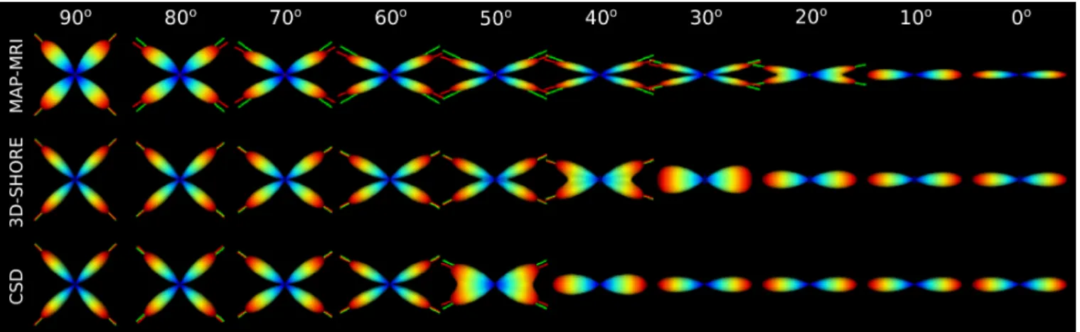
Fig. 1: ODFS of a noiseless multi-tensor crossing obtained using either MAP-MRI with basis order 6, 3D-SHORE with basis order 8 or CSD with spherical harmonics order 8 using only 60 samples. When a crossing is detected, the ground truth and the estimated fiber directions are shown as green and red lines. As you can see, MAP-MRI is able to resolve much smaller crossing angles than the other techniques, but also consistently underestimates the crossing angles smaller than 90 degrees.
where Raniso scales the anisotropy. Setting Raniso = 1 or
Raniso= 0 sets the fitting to either MAP-MRI or 3D-SHORE.
For arbitrary Raniso we fit the basis coefficients c to
the data y = E(q) using regularized least-squares as c = argmincky − Qck2 + λ R(c) where design matrix Q ∈
RNdata×Ncoef has elements Q
ij = ΦNi(A, qj), with qj the
q-space positions of the data. For R(c) we choose Laplacian regularization of the MAP-MRI basis [4] and use generalized cross-validation to find the regularization weight λ [5].
As the fitted basis coefficients linearly describe both the signal E(q) and the diffusion propagator P (r), where r de-fines the real displacement vector of a diffusing particle, they also linearly describe the Orientation Displacement (ODF) as
ODFs(v) = Z ∞ 0 rsP (rv)dr = Nmax X i=0 ciΩi(A). (3)
Here r = vr with v an orientation on the unit sphere, s is the radial moment which induces a sharpening effect on the ODF (s = 2 gives the marginal ODF), and Ω is the ODF basis function. The closed form of Ω can be found in [2]. Throughout this paper we use s = 6 to retrieve ODF maxima.
2.2. Estimation of Scalar Quantities
From the fitted MAP-MRI coefficients we compute scalar indices known as the Return-to-Origin and Return-to-Axis Probabilities (RTOP and RTAP) [2]. In a given diffusion time, RTOP is defined as the probability that a spin does not have a net displacement (i.e. P (0)) and RTAP as the inte-grated probability that a spin diffuses along the axis of the axons, here defined as the main tensor eigenvector Rk. When
we represent axons are parallel cylinders we can relate RTAP to the mean cross-sectional area (MCSA) of the axons, from which we can then compute the mean axon radius [2].
However, this relation only holds if only the intra-axonal signal is considered, short gradient pulses are used (δ ≈ 0) and long diffusion times are used (∆ δ) [6]. If these conditions are met we compute the axon radii as hRi =p1/(RTAP π) with RT AP = R
RP (Rkr)dr
3. RESULTS
Using synthetic data we investigate (I) the effect of MAP-MRI’s anisotropic basis functions, (II) the angular recovery accuracy of 3D-SHORE, (III) the effect sampling data on multiple shells rather than a single shell and (IV) the effect truncating acquisitions on angle and axon radius recovery. We then use human data from the WU-Minn Human Connec-tome Project (HCP) [7] to investigate the effect truncating the data has on RTOP recovery.
3.1. Synthetic Results
In experiment (I) we generate fiber crossings with angles ranging from 00to 900using the multi-tensor model in Dipy [8]. The tensor eigenvalues are {λx, λy, λz} = {1.7, 0.2, 0.2}
e − 3, and we sample 60 samples spread evenly over 3 shells at b = {1000; 2000; 3000} s/mm2 [9]. In Fig. 1 we show ODFs computed using MAP-MRI, 3D-SHORE and as a ref-erence Constrained Spherical Deconvolution (CSD) [10]. We observe that MAP-MRI is able to resolve smaller crossings but also consistently underestimates the crossing angle.
We quantify this effect using Eq. (2) to scale Raniso
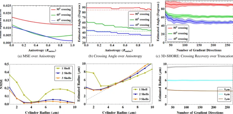
be-tween 0 (3D-SHORE) to 1 (MAP-MRI). Using a basis order of 8, we compute the mean squared signal reconstruction er-ror (MSE) and estimate the crossing angle using the ODF on a 450, 600and 900 fiber crossing. We observe that as Raniso
increases the MSE decreases (Fig. 2a) but the crossing under-estimation increases (Fig. 2b), which corresponds with Fig.
(a) MSE over Anisotropy (b) Crossing Angle over Anisotropy (c) 3D-SHORE: Crossing Recovery over Truncation
(d) MAP-MRI: Multi-Shell effect MSE (e) MAP-MRI: Multi-Shell effect Radius Estimation (f) MAP-MRI: Radius Recovery over Truncation Fig. 2: Synthetic experiment results. In (a) and (b) we investigate the effect of MAP-MRI’s basis anisotropy on signal re-construction error and crossing angle recovery. In (c) we show the robustness of crossing angle recovery over the number of sampled gradient directions. In (d) and (e) we show the result of sampling on multiple shell on signal reconstruction and axon radius recovery. Finally (f) shows the robustness of axon radius recovery over the number of sampled gradient directions.
1. These results show that MAP-MRI is better suited for sig-nal reconstruction and 3D-SHORE for angle recovery.
In experiment (II) we compare the angular accuracy of CSD and 3D-SHORE on tractography. We used the Trac-tometer evaluation system [11] on the synthetic ISBI 2013 reconstruction challenge data set [12] to compare tractogra-phy performances (SN R = 10, 20, 30). Tractogratractogra-phy was obtained for CSD (60 samples, one shell at b = 3000 s/mm2) and 3D-SHORE (60 samples, spread evenly over 3 shells at b = {1000; 2000; 3000} s/mm2) using the Dipy [8] EuDX deterministic tractography. EuDX tractography uses only the ODF maxima to propagate streamlines [8], and thus, is suit-able to compare angular accuracy through tractography. We find that CSD and 3D-SHORE obtain similar results (Table not shown due to space limitations) on the Tractometer met-rics [11], which is consistent with experiment (I).
We then study the effect of spreading the same number of samples over multiple sampling shells (III) using MAP-MRI. We use the cylinder model [3], which respects the conditions stated in Section 2.2, and sample 60 samples on either 1, 2 or 3 shells (bmax = 3000 s/mm2) for different cylinder (axon)
radii. We find that sampling over more shells decreases the MSE of the signal fitting (Fig. 2d) and allows for the recovery of smaller axon radii (Fig. 2e).
Finally in experiment (IV), we study how many samples we need to robustly recover crossing angles using 3D-SHORE
and recover axon radii using MAP-MRI. As in the Human Connectome Project data, for both we sample 270 samples over the same 3 b-shells and add noise 300 separate times such that SN R = 20. We then increasingly truncate the data, making sure the sampling distribution remains uniform [9], and compute the means and standard deviations of the recov-ered crossing angles (Fig. 2c) and axon radii (Fig. 2f). In Fig. 2c we see that all three crossings can be robustly estimated until we use less than 100 samples, at which point the small-est 450 crossing becomes difficult to recover. In Fig. 2f we see that MAP-MRI robustly recovers the chosen axon radii despite truncation to even 30 gradient directions.
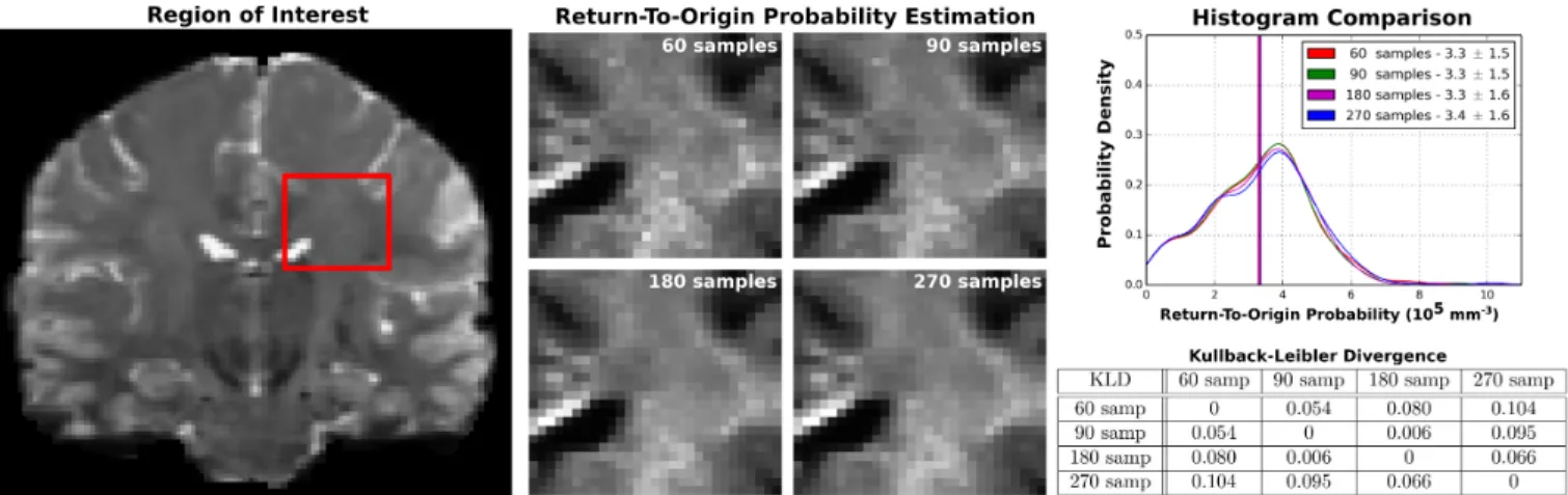
3.2. Human Connectome Project: RTOP Recovery We use the WU-Minn HCP data [7] to quantify the robustness of estimating RTOP using MAP-MRI on increasingly under-sampled data. The full HCP data has b-values {0; 1,000; 2000; 3,000} mm/s2 with {18; 90; 90; 90} gradient direc-tions, ordered as in [9] such that subsets of the first N samples are still isotropic. We select a region of interest near the cor-pus callosum (Fig. 3) and compute RTOP using 270, 180, 90 and 60 samples. We see that RTOP’s white matter contrast is very similar even between 270 and 60 samples. We verify this by showing histograms of RTOP and the Kullback-Leibler di-vergence. Both confirm the similarity in RTOP values.
Fig. 3: Human Connectome Project (HCP) experiment results. We select a region of interest near the corpus callosum in the b0 image (left). Using MAP-MRI we compute RTOP in this area, where we increasingly truncate the data from the full 270 to just 60 gradient directions. Visually the RTOP value remain very similar despite truncation (middle). We verify their similarity with histograms of the RTOP values (top right) and by computing the Kullback-Leibler divergence (bottom right).
4. DISCUSSION AND RESULTS
In this paper we showed that with just 60 sampled gradient directions, spread over 3 b-shells, we can accurately estimate both the directionality and microstructural measures of white matter tissue. We provided a way to scale the anisotropy of MAP-MRI’s basis functions and quantified a consistent bias that MAP-MRI underestimates crossing angles under 900as
the anisotropy in its basis functions increases. Despite of this bias, we showed on both synthetic and human data from the Human Connectome Project that by using a mixed ap-proach of 3D-SHORE for angle recovery and MAP-MRI for microstructure recovery we obtain the best results.
Acknowledgments
Data were provided [in part] by the Human Connectome Project, WU-Minn Consortium (Principal Investigators: David Van Essen and Kamil Ugurbil; 1U54MH091657) funded by the 16 NIH Institutes and Centers that support the NIH Blueprint for Neuroscience Research; and by the McDonnell Center for Systems Neuroscience at Washington University. This work was partly supported by the French ANR ”MOSIFAH” under ANR-13-MONU-0009-01.
5. REFERENCES
[1] Stejskal. ”Use of Spin Echoes in a Pulsed Magnetic-Field Gradient Study Anisotropic Restricted Diffusion Flow.” J CHEM PHYS 43.10, pp. 3597-3603, 1965.
[2] ¨Ozarslan et al. ”Mean Apparent Propagator (MAP) MRI: A novel Diffusion Imaging Method for Mapping Tissue Microstructure.” NeuroImage 78, pp. 16-32, 2013.
[3] ¨Ozarslan et al. ”Simple Harmonic Oscillator Based Re-construction and Estimation for One-Dimensional q-Space Magnetic Resonance (1D-SHORE)” Excursions in Harmonic Analysis, Volume 2 pp. 373-399, 2013. [4] Fick et al. ”Laplacian-Regularized MAP-MRI:
Improv-ing Axonal Caliber Estimation”. ISBI 2015.
[5] Craven et al. ”Smoothing Noisy Data with Spline Func-tions.” NUMER MATH 31.4, pp. 377-403, 1978. [6] Bar-Shir et al. ”The effect of the diffusion time and pulse
gradient duration ratio on the diffraction pattern and the structural information estimated from q-space diffusion MR: Experiments and simulations.” J MAGN RESON 194.2, pp. 230-236, 2008.
[7] Van Essen et al. ”The WU-Minn Human Connectome Project: An overview.” NeuroImage 80, pp. 62-79, 2013. [8] Garyfallidis et al. ”Dipy, a library for the analysis of diffu-sion MRI data.” Front. Neuroinform., vol.8, no.8. (2014). [9] Caruyer et al. ”Design of multishell sampling schemes with uniform coverage in diffusion MRI”. MAG RESON MED, 69(6), pp. 1534-1540, 2013.
[10] Tournier et al. ”Robust determination of the fibre orien-tation distribution in diffusion MRI: non-negativity con-strained super-resolved spherical deconvolution.” Neu-roImage 35.4, pp. 1459-1472. 2007.
[11] Cˆot´e et al Tractometer: Towards Validation of Tractog-raphy Pipelines, Medical Image Analysis, vol. 17, no. 7, pp. 844857, 2013.
[12] Caruyer et al. ”Phantomas: a flexible software library to simulate diffusion MR phantoms.” ISMRM 2014, 2014.