Combining Laboratory and Field Data in Rail Fatigue Analysis
byFeng-Yeu Shyr
B.S., National Taiwan University (1985)
M.S., National Taiwan University (1987)
Submitted to the Department of Civil Engineering
in Partial Fulfillment of the Requirements for the Degree of
Doctor of Philosophy
in Transportation Systemsat the
Massachusetts Institute of Technology
August 1993© Massachusetts Institute of Technology, 1993, All rights reserved
Signature of Author
Department of tivil and Environmental Engineering August 31, 1993
Certified
by '
Moshe E. Ben-Akiva Professor of Civil and Environmental Engineering
Thesis Supervisor
Accepted by
-Eduardo Kausel
Departmental Committee on Graduate Students
ACNEiVE$
MASSA CHLISE' !fNSTIUTECombining Laboratory and Field Data in Rail Fatigue Analysis
byFeng-Yeu Shyr
Submitted to the Department of Civil and Environmental Engineering on August 31, 1993 in partial fulfillment of the requirements for the Degree of Doctor of Philosophy in Transportation Systems
Abstract
Rail fatigue is one of the key factors affecting rail service life. Once a defected rail was detected, it will be replaced immediately to avoid derailment. Fatigue failures cost railroads in various aspects such as repairs, traffic delays, and accidents, and also have an impact on the reliability of rail service. The purpose of rail fatigue analysis is to provide assessment of maintenance and operations strategies in regard to rail fatigue.
Because the field data regarding rail fatigue are often limited, the model calibrated based on field data may not be reliable for predicting future deterioration conditions. In addition, the field data may be measured with error and subject to temporal correlation. Therefore, the Phoenix model which has been developed based on theories of material behavior and laboratory results was used as a supplemental tool to analyze rail fatigue. The data generated from the Phoenix model does not have the disadvantages as those in the field data. However, the Phoenix model has not yet been validated by the field data and the results could be biased. Thus, the goal of this research is to develop a reliable rail fatigue model by combining both data sources.
Assuming no spatial correlation among defects, the rail fatigue model was formulated as a spatial Poisson with a defe t occurrence rate which depends on the usage of rail and factors affecting fatigue. The defect rate was also formulated to incorporate multiple failure types and dynamic explanatory variables.
The model parameters calibrated to the Phoenix output and to the field data were both in agreement with the a priori expectation of fatigue behavior. By assuming that the Phoenix model was biased, the unbiased parameters for the combined model and the biases were simultaneously estimated by pooling both data sources.
Finally, this research applies the combined model to analyze the effects of maintenance and operation practices regarding fatigue failures.
Thesis supervisor: Dr. Moshe E. Ben-Akiva
Acknowledgments
I am grateful for the financial support and the data provided by the Association of American Railroads.
I sincerely thank Professor Moshe Ben-Akiva who supervised this research and provided helpful suggestions and insightful directions in writing this thesis. I also thank other committee members, Professor Haris Koutsopoulos, Professor David Bernstein, and Carl Martland for valuable comments to the research. In addition, I would like to express my personal gratitude especially to Carl Martland for his beneficial guidance and remarks regarding to railroad operations and maintenance.
Furthermore, I would like to thank Roger Steele who provided useful insight to the Phoenix model and to Carlo Fraticelli who provided empirical data to this research.
I appreciate the help from Peter Silberman and Amalia Polydoropoulou in correcting the draft of this thesis. I learned a lot from the discussions with Ted Botimer and Dinesh Gopinath for the presentation of my doctoral seminar and for using Gauss and Maxlik to estimate the model.
I also want to thank my best friend, Shangyao Yan, for the cheerful experiences that we both shared in studying and traveling. Without his encouragement and support, this thesis would not exist. Our friendship is "like a bridge over troubled water".
Finally, I would like to extend my sincere gratitude to my parents for their understanding and endless support to their only son during my stay at MIT.
Table of Content
Chapter 1: Introduction ... 11
1.1 Motivation ... ... 11
1.2 Research Objectives and Scope ... ... 18
1.3 Thesis O utline ... 20
Chapter 2: Review of Rail Fatigue Analysis ... 23
2.1 Causes of Fatigue Failures and Factors Affecting Rail Defects ... 23
2.2 An Existing Engineering Model - The Phoenix Model ... 27
2.3 Current Statistical Approaches to Rail Fatigue Analysis ... 31
Chapter 3: Review of Data Combination, Measurement Error and Temporal
Correlation Methods ...
...
... 38
3.1 Methods for Data Combination ... 38
3.1.1 Bayesian Updating Method ... ... 38
3.1.2 Combined Transfer Estimator (CTE) ...
42
3.1.3 Joinz Estimation ... 43
3.2 Applications of Data Combination Methods ... 45
3.3 Methods for Measurement Error and Temporal Correlation ... 47
Chapter 4: Rail Fatigue Model... 50
4.1 Model with Multiple Types of Failures... 50
4.2 Aggregation Over Usage Period and Space . ... 58
4.2.1 Hazard Rate for a Discrete Usage Period ... 58
4.2.2 A Spatial Rail Fatigue Model ... 59
4.2.3 Spatial Poisson Model with Multiple Types of Defects ... 62
4.3 Specification of Functional Form ... ... 67
4.3.1 Stochastic Threshold for Defect Regimes ... ... 67
4.3.2 Model with Dynamic Explanatory Variables . ... 68
4.3.3 Inclusion of Failure Distributions ... 71
4.4 Summary ...
74
Chapter 5: Data Collection and Analysis
...
76
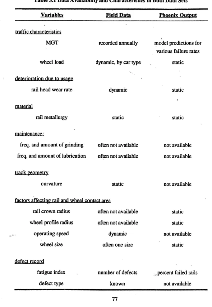
5.1 Assessment of Data Availability and Characteristics ...:... 76
5.2 Description of Collected Data ...
79
5.2.1 Generation of Phoenix Data ... 79
5.2.2 Acquisition of Field Data ... ... 80
5.3 Model Formulation for Different Data Sources ...
...
82
5.4 Data Statistics ...
86
5.4.1 Descriptive Statistics ... 86
5.4.2 Correlation Statistics ...
88
5.4.3 Defect Pattern in the Field Data .... ... 92
Chapter 6: Estimation Approach and Results . ... 117
6.1 Separate Estimation ... 117
6.1.1 Phoenix Data Model ... 117
6.1.2 Field Data Model ...
126
6.1.3 Testing Temporal Correlation in the Field Data ... 131
6.1.4 Testing Measurement Errors in Field Data ... 134
6.1.5 Comparison of Phoenix and Field Data Estimation Results ... 139
6.2 Joint Estimation... 143
6.3 Comparison of Model Predictions ... 149
7.1 Prediction of Defec Rates and Probability of Risk ... 156
7.2 Sensitivity Analysis of Wheel Loads on Defects ... 158
7.3 Evaluation of Grinding Effectiveness ... ... ... 161
7.4 Sensitivity Analysis of Other Factors ... 165
7.5 Sum m ary... ... 1... 171
Chapter 8: Conclusion ...
172
8.1 Research Summary ... ... 172
8.2 Contributions ... 176
8.3 Future Research Directions ... ... 178
Appendix A: Properties for Hazard Rate and Survival Function ... 181
Appendix B: Birnbaum-Saunders Fatigue Life Distribution ... 182
Appendix C: Failure Distributions for Survival Analysis ... 183
Appendix D: Least Square Estimate with Measurement Error ... 184
Appendix E: Reviews of Measurement Error and Temporal Correlation ... 185
Appendix F: Data Combination Methods for a Linear Deterioration Model ... 189
Appendix G: First-Order Conditions for the Estimation of the Phoenix Data
Model ...
191
Appendix H: Field Data Processing ... 193
List of Figures
Figure 1.1: Relationships Among Deterioration, Maintenance, and Operations ... 13
Figure 1.2: Generation Processes for the Laboratory Data and the Field Data ... 15
Figure 2.1: Transverse, Horizontal, and Vertical Planes for Rail Head ... 24
Figure 2.2: Contact Rail Crown Radius and Wheel Profile Radius:... 26
Figure 2.3: Aggregated S/N Curves ... 28
Figure 2.4: Aggregation of Defect Records Over Cumulative 'MGT ... 35
Figure 2.5: Distribution Fitting Against Cumulative MGT ... 36
Figure 4.1: Defect Pattern for Two Defect Types in Model 1 ... 56
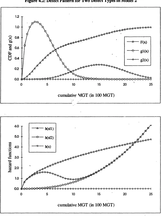
Figure 4.2: Defect Pattern for Two Defect Types in Model 2 ... 57
Figure 5.la: Defect Pattern for Division 402 on Segment A ... 95
Figure 5.lb: Defect Pattern for Division 402 on Segment B ... 96
Figure 5. lc: Defect Pattern for Division 402 on Segment C ... 97
Figure 5. ld: Defect Pattern for Division 402 on Segment D ... 98
Figure 5.2a: Defect Pattern for Division 607 on Segment A ... 99
Figure 5.2b: Defect Pattern for Division 607 on Segment B ... 100
Figure 5.2c: Defect Pattern for Division 60}7 on Segment C ... 101
Figure 5.3a: Defect Pattern for Division 681 on Segment A ... 1()2 Figure 5.3b: Defect Pattern for Division 681 on Segment B ... 103
Figure 5.3c: Defect Pattern for Division 681 on Segment C ... 104
Figure 5.4a: Defect Pattern for Division 613 on Segment A ... 105
Figure 5.4b: Defect Pattern for Division 613 on Segment B ... 106
Figure 5.4c: Defect Pattern for Division 613 on Segment C ... 1... 107
Figure 5.4d: Defect Pattern for Division 613 on Segment D ... 108
Figure 5.4e: Defect Pattern for Division 613 on Segment E ... 109
Figure 5.4g: Defect Pattern for Division 613 on Segment G ... 1 11
Figure 5.4h: Defect Pattern for Division 613 on Segment H ... 112
Figure 5.5a: Defect Pattern for Division 684 on Segment A ... 113
Figure 5.5b: Defect Pattern for Division 684 on Segment B ... 114
Figure 5.5c: Defect Pattern for Division 684 on Segment C ... 115
Figure 5.5d: Defect Pattern for Division 684 on Segment D ... 116
Figure 6.1a: Comparison of Fatigue Defect Rates Predicted by Different Models ... 150
Figure 6. lb: Comparison of TD Defect Rates Predicted by Different Models ... .. 151
Figure 6. Ic: Comparison of SH Defect Rates Predicted by Different Models ... .. 151
Figure 6.2a: Comparison of Model Predictions with Field Data for Division 6(07 ... 153
Figure 6.2b: Comparison of Model Predictions with Field Data for Division 613 ... 154
Figure 6.2c: Comparison of Model Predictions with Field Data for Division 684 ... 155
Figure 7.1 la: Fatigue Defect Rates for Various Wheel Loads ... 159
Figure 7.lb: TD Defect Rates for Various Wheel Loads ... 160
Figure 7.1c: SH Defect Rates for Various Wheel Loads ... 160
Figure 7.2a: Fatigue Defect Rates for Various Grinding Practices ... 162
Figure 7.2b: TD Defect Rates for Various Grinding Practices ... 162
Figure 7.2c: SH Defect Rates for Various Grinding Practices ... 163
Figure 7.3a: Fatigue Defect Rates for Various Contact Profiles ... 163
Figure 7.3b: TD Defect Rates for Various Contact Profiles ... 164
Figure 7.3c: SH Defect Rates for Various Contact Profiles ... 164
Figure 7.4a: Fatigue Defect Rates for Various Speeds ... 166
Figure 7.4b: TD Defect Rates for Various Speeds ... 167
Figure 7.4c: SH Defect Rates for Various Speeds ... 167
Figure 7.5a: Fatigue Defect Rates for Various Rail Hardness ... 168
Figure 7.5b: TD Defect Rates for Various Rail Hardness ... 168
Figure 7.6a: Fatigue Defect Rates for Various Rail Weights ... 169 Figure 7.6b: TD Defect Rates for Various Rail Weights ... 170 Figure 7.6c: SH Defect Rates for Various Rail Weights ... 170
List of Tables
Table 1.1: Characteristics of Field Data and Laboratory Data ... 1... 17
Table 5.1: Data Availability and Characteristics in Both Data Sets ... 77
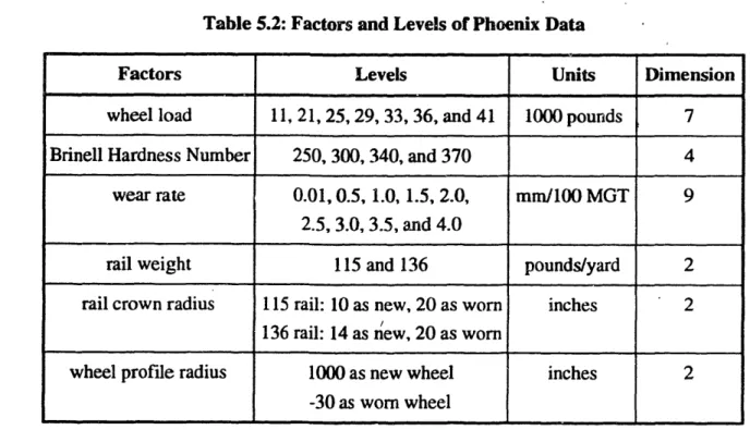
Table 5.2: Factors and Levels of Phoenix Data ...
...
...
80
Table 5.3: Descriptive Statistics of the Phoenix Model Output ...
87
Table 5.4: Descriptive Statistics of the Field Data .
...
89
Table 5.5: The Correlation Matrix of the Phoenix Data ...
....
...
90
Table 5.6: The Correlation Matrix of the Field Data ...
91
Table 6.1: The Correlation Among Explanatory Variables of the Phoenix Data ... 123
Table 6.2: Estimated Coefficients for Phoenix Model Output ... ... 125
Table 6.3: The Correlation Among Explanatory Variables of the Field Data ... 129
Table 6.4: Estimated Coefficients for Field Data ... 130
Table 6.5: Estimated Results with Stochastic Temporal Correlation ... 135
Table 6.6: Estimated Results with Temporal Correlation and Measurement Error ... 138
Table 6.7: Comparison of Estimation Results from both Data Sets - Model 1
... 140
Table 6.8: Comparison of Estimation Results from both Data Sets - Model 2 ... 141
Chapter 1: Introduction
1.1 Motivation
This study is motivated by the recent development of data combination techniques and the need for a reliable rail fatigue model. Data combination has been widely applied to areas in which the data drawn from the field or from the history are often limited and therefore empirical analysis based purely on these data would be unreliable. Thus, supplemental data are generated to provide a better understanding of the problem in
context.
For example, in demand forecasting and market research, revealed preferences (RP) data, which represent actual demand, are often limited in the ranges of variable values. As a result, in some cases models calibrated from RP data may not be sufficiently reliable for
demand forecasting. Therefore, stated prefereaces (SP) data collected from consumer
surveys are often used as supplemental data to study demand behavior. However, SP data may be biased because the survey responses do not reflect actual behavior. Data combination techniques have been developed to reconcile the differences between oihtypes of data to obtain more reliable model parameters.
There have been several applications of data combination techniques to transportation studies. In particular, this research builds on a stream of studies at MIT that began during the mid 1970's. Atherton and Ben-Akiva [1976] applied a Bayesian data combination techniques to transfer and update disaggregate travel demand models. Ben-Akiva [1987] developed the framework for combining multiple sources of data to estimate origin-destination matrices. Ben-Aklva and Bolduc [1987] extended the Bayesian approach for transferring model parameters. Morikawa [1989] developed the methodology to combine SP and RP data for travel demand analysis; Vieira [1992] also applied SP and RP data
combination techniques to study the value of service in freight transportation. The only previous application of data combination to rail fatigue analysis is the work of Campodonico [1992]. She calibrated a rail fatigue model using a Bayesian procedure that combined field observations with the output of a theoretical rail fatigue model to predict rail fatigue defect rates.
The Need for a Reliable Rail Fatigue Model
According to Railroad Facts published by the Association of American Railroads [1987], the railroad industry spent more than 4 billion dollars each year in the last decade to maintain tracks at an adequate operational level. The maintenance of infrastructure accounts for 40% of railroad industry's maintenance budget, about 18% of overall operating expenses. Since rail is the most expensive component of a railway, it has always been a great concern of the railroad industry to search for the most effective strategies of maintaining rail.
The service life of a rail is determined by two deterioration indices, the level of rail wear, and the rate of fatigue failure, namely, defects per mile per year. Fatigue defects, if not detected and replaced, can lead to broken rails that may cause derailments. However, the true mechanism of rail fatigue is still unknown. As a result, it is very difficult to predict fatigue failure accurately.
For safety and economic reasons, a stretch of rail should be replaced when the expected rate of fatigue failures exceeds a certain tolerance level. In other words, a stretch of rail reaches its fatigue service life limit when it is more economical and safer to replace the rail than to leave it in service. Therefore, the purpose of rail fatigue analysis is to predict the rate of fatigue defects.
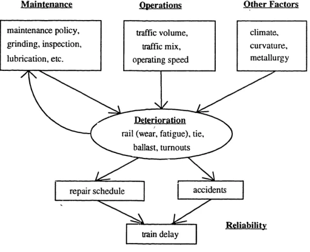
As shown in Figure 1.1, the deterioration level of a railroad component is affected by: 1) maintenance policy, such as frequency of grinding, lubrication, and inspection; 2) operating conditions, such as traffic composition, traffic volume, and speed; and 3) other factors such as materials selected for installation and replacement, track geometry (curvature and grade) and climate. Any failure in a railroad component will have an impact on the schedule of repair and, if not detected, will increase the chance of accidents. Both accidents and repairs cause train delays and affect service reliability.
Maintenance
Operations
Other Factors
Figure 1.1: Relationships Among Deterioration, Maintenance, and Operations
In addition to the above factors, rail fatigue failure will also be affected by the deterioration levels of other railroad components, such as ties and ballast, and the amount
of rail head wear. This is because fatigue failure is affected by the dynamic wheel load applied to the rail and the contact stresses between rail crown and wheel [Steele, 1988]. Since the dynamic wheel load depends on the foundation strength and operating speed, the deterioration of ties and ballast affect the foundation strength and thus affect rail fatigue. Meanwhile, rail wear changes the shape of the rail head and the contact area between rail crown and wheel and thus affect the contact stresses.
The purpose of rail fatigue analysis is to capture or model the underlying relationships among fatigue failures, the operating environment, maintenance activities, and rail metallurgy in order to select the most efficient maintenance and operations strategies.
The Need for Data Combination in Rail Fatigue Analysis
In general, field data for the studies of deterioration behavior is often limited, since it takes a long period of time to collect enough failed samples. Therefore, instead of only analyzing field observations, laboratory experiments are conducted to generate supplemental data for rail deterioration studies.
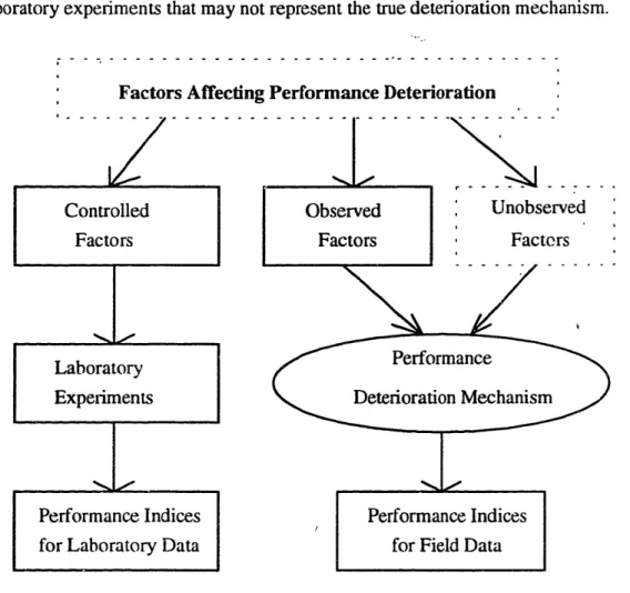
Figure 1.2 highlights the differences in the data generation processes between field and laboratory data. The dotted-line rectangles represent the unknown attributes while solid rectangles stand for known attributes; the oval represents the unknown relationship between performance indices and deterioration related factors. Performance indices are
measures of deterioration, such as defects per mile in the rail fatigue analysis. As shown in Figure 1.2, field data contain information of observed. factors affecting deterioration and performance indices, while the laboratory data consists of controlled factors and performance indices produced by laboratory experiments. Therefore, the differences between the field data and the laboratory data are two-fold: 1) the observed factors in the field data may not be the same as the controlled factors in the laboratory data; 2) the
mechanism while the performance indices in the laboratory data are the output of laboratory experiments that may not represent the true deterioration mechanism.
Factors Affecting Performance Deterioration
Cont
Factrolled tors
Figure 1.2: Generation Processes for the Laboratory Data
and the Field Data
The factors affecting deterioration may not be fully captured in the field data due to limited knowledge of deterioration mechanism or the difficulty in data collection. Since the factors affecting rail fatigue and the performance indices are collected over time in different locations, the data are therefore referred to as pooled time-series and cross-section data.
Because the ranges of observed factors in the field data are usually limited, a rail deterioration model calibrated on the field data may not be able to reflect the effects of
Laboratory
Experiments
_
Performance Indices
for Laboratory Data
_ -
changes in maintenance actions and operations practices on deterioration conditions. Moreover, the observed factors may be highly correlated, for instance, high traffic density lines often use stronger rails and are well-maintained. A multi-collinearity problem in field data may result in inaccurate model.
Since the field data consist of time-series and cross-sectional 'observations, there is a
need to consider temporal correlation [Greene, pp. 481, 1990]. This study will enhance existing methods for dealing with temporal correlation in ithe estimation of the deterioration model that uses field data. The causes of the temporal correlation and the methods for solving this problem will be discussed in Chapters 3 and 6.Furthermore, the observed factors may not be accurately measured in the field data. The existence of measurement errors also affects the accuracy of model estimation [Greene, pp. 294, 1990]. Therefore, methods used for correcting measurement errors are required to estimate a rail deterioration model using field data. Details of measurement error problem will also be discussed in Chapters 3 and 6.
Ideally, in the laboratory, we would like to exactly replicate the true deterioration process for rail fatigue. Unfortunately, there are many factors in the deterioration process, such as aging of material, dynamic loading effects under various speeds and curvatures,
and climate which are too complicated to reproduce. The result of our inability to
replicate the true deterioration process is biased laboratory data.
However, compared to field data, laboratory data has the following advantages: 1) the controlled factors can be varied at larger ranges of values with alternate combinations to reduce correlation and to avoid multi-collinearity; 2) the controlled factors are free of measurement errors; and 3) laboratory data are free of temporal correlation since all
experiments are independently conducted. The characteristics of both types of data are
Currently, two types of data are used for rail fatigue analysis, data collected from actual defective sites, and data generated from a fatigue model called the Phoenix model. The Phoenix model was developed by the Association of American Railroads [Steele, 1990] and is based on material behavior theories and results from laboratory experiments of rail fatigue behavior. Therefore, the data produced by the Phoenix model represent material properties of rail captured in laboratory experiments.
Table 1.1: Characteristics of Field Data and Laboratory data
Field Data
Laboratory data
- observed factors may be measured
with error
- observed performance indices may be subjected to temporal correlation
- ranges of observed factors are limited
- observed factors may e highly
correlated
- explanatory variables may change ove time
-controlled factors have no
measurement error
- derived performance indices may be biased
- controlled factors can be specified ai
larger ranges- controlled factors can be specified ft all possible combinations
r - explanatory variables are in
steady-state
The Phoenix model simulates the microscopic processes leading to the initiation and growth of fatigue defects in the rail head. The Phoenix model predicts rail fatigue life under various conditions. A detailed description of the Phoenix model is included in Chapter 2.
__
_.
t
Since the Phoenix model has only been validated by very limited data obtained from railroad testing facilities, not by field data, the calibration of a rail fatigue model using both types of data will identify possible biases in the Phoenix model.
In conclusion, the purpose of applying data combination techniques in rail fatigue analysis is to identify the differences and similarities between the two types of data, and to utilize the advantages of both types of data in order to calibrate t relationship between performance indices and the factors affecting fatigue more accurately.
1.2 Research Objectives and Scope
The objectives of this study are the following:
1. Development of a comprehensive rail fatigue model.
The formulation of the rail fatigue model will be based on extant models for fatigue failure and survival analysis. The model will incorporate the following features:
i) Duration of rail usage and fatigue failures
-Since a rail must be replaced if defective, by definition, the observed probability of failure, given that a rail is still in use, is a hazard rate. The model will incorporate hazard rate models which are usually used for fatigue analysis. A detailed review of literature and statistical methods that deal with fatigue analysis is presented in Chapter 2.
ii) Different patterns for different types of failures
-The mechanism of each type of failure may be different. As a result, the rail fatigue model will take into account the different patterns for different types of failures.
iii) Spatial correlation and aggregation of fatigue defects
-Most of the rails currently used in North America are continuously welded. Therefore, the spatial correlation among defects should be considered in the rail fatigue model. Meanwhile, rail defect data often contain hundreds of miles of track (about a hundred thousand rails); as a result, a spatial model is needed to
aggregate rails into homogenous segments to reduce computational requirements
without the loss of information.iv) Dynamic effects of fatigue related factors
-Since the rail fatigue related factors in the field data are changing pver time, the model will be formulated to incorporate the dynamic effects of these factors. The steady state of input variables in the laboratory data is a special case.
2. Incorporation of measurement error and temporal correlation in the field data.
Since the presence of measurement errors and temporal correlation will affect estimated parameters from field data, specific models accounting for measurement errors and temporal correlation will be developed.
3. Comparison of rail fatigue models estimated using field data and Phoenix model data
The purpose of the comparison is to determine the differences as well as the similarities between the two sets of model parameters estimated from two data sources.
The application of data combination is to seek for estimates of parameters with smaller
variances. For example, if explanatory variables in the field data are lack of variability that result in high variances of estimated parameters while the laboratory data provides more reliable estimates, then data combination methods can be applied to obtain more efficient model parameters. Data combination can also identify the biases in some data sources.
different, then by specifying the biases in different data sources, the true parameters and the biases can be jointly estimated by using the joint estimation method.
4. Validation of the Phoenix model.
The predictions from the Phoenix model may be biased because the true. fatigue mechanism may not be fully captured by the Phoenix model. As a result, the estimated parameters using the Phoenix data may be significantly different from the estimated parameters using the field data. Therefore, the parameters that capture the bias will be specified in the combined model and will be estimated by pooling both field and Phoenix data. The detailed approach regarding the estimation of the combined model is described in Chapter 6.
5. Evaluation of maintenance and operation practices.
The ultimate purposes of the model is to provide a tool for the assessment of railroad maintenance practices and strategic operations planning. The evaluation will be done by performing sensitivity analyses of fatigue defect rates on maintenance and operations activities using the calibrated fatigue model.
1.3 Thesis Outline
Given the objectives described above, the contributions of this study are two-fold:
1) Methodology
The development of a comprehensive statistical rail fatigue model will incorporate all related models for four aspects of the rail fatigue model described above. Since the fatigue model developed in this study is a general framework, it can also be used for the analyses of other deterioration studies. In addition, this study will enhance existing
methods for delaing with measurement error and temporal correlation in the estimation of the deterioration model that uses field data. Finally, this study will propose the methodology for combining laboratory and field data to estimate a statistical rail fatigue model.
2) Rail Fatigue Analysis
Because the current model used for rail fatigue analysis, namely, the Phoenix model, has not been validated by the field observations, it is a great concern for the railroads to verify the Phoenix model. By implementing data combination of the Phoenix output and the field data, this study will identify the potential bias in the Phoenix model. In addition, this research will demonstrate the applications of the calibrated fatigue model to evaluate operations and maintenance practices and to predict future fatigue deterioration.
The highlights of each chapter are as follows:
Chapter 2 reviews the background fof fatigue analysis, including both laboratory approaches and statistical methods. A detailed description of the causes of rail fatigue failure is also discussed. Furthermore, Appendices A, B and C review the most commonly used fatigue failure distributions and basic properties of failure functions.
Chapter 3 reviews the methods for data combination and proposes estimation approaches to identify measurement errors and temporal correlation in the field data. In addition, Appendix E reviews methods used for measurement error and temporal correlation. -Meover, in the case in which the relationship between the deterioration
indices and explanatory variables can be formulated as a linear model, a data combination method for the linear model is also proposed in Appendix F.
defects; 3) spatial aggregation of defect occurrences; and 4) dynamic effects of explanatory variables. Finally, this chapter proposes the specifications for the rail fatigue model.
Chapter 5 describes: 1) data requirements for rail fatigue analysis; 2) procedures for the generation of laboratory data; 3) content of the acquired data and model formulations
for both data sources; and 4) descriptive statistics and correlation analyses of both data
sets. The procedures of data processing for the field data are shown in Appendix H.
Chapter 6 proposes the estimation methods for separate and joint estimation and discusses the obtained results. The estimation of the field data model with the presence of measurement errors and temporal correlation is presented. Finally, this chapter compares the defect patterns predicted by the field data model, the laboratory data model, and the combined model.
Chapter 7 applies the calibrated model to predict the annual failure rate, to calculate the probability of risk for exceeding the maximum allowable failure rate, and to evaluate the effects of maintenance and operations practices on fatigue failures.
Finally, Chapter 8 summarizes the conclusions and contributions of this study and suggests areas for future research.
Chapter 2: Review of Rail Fatigue Analysis
This chapter first describes the causes of fatigue failure, the factors affecting rail fatigue defects4 and the fundamental relationships between rail fatigue and some of these factors; then an existing engineering model, the Phoenix model, is presented as an example of analyzing fatigue behavior using laboratory data and basic material properties regarding fatigue; finally, existing statistical methods used to model rail fatigue failure are reviewed.
2.1 Causes of Fatigue Failures and Factors Affecting Rail Defects
Fatigue failure is initiated by the imperfection of materials or from small cracks inside the material. Cracks grow due to repeated loads applied to the material. Regarding the formation of small cracks, Broek [1986, pp. 48] explains the phenomenon as follows:
"Under the action of cyclic loads cracks can be initiated as a result of cyclic plastic deformation. Even if the normal stresses are well below the elastic limit, locally the stresses may be above the yield due to stresses concentrations at inclusions or mechanical notches. Consequently, plastic deformation occurs locally on a microscale, but it is insufficient to show in engineering terms".
As for rail fatigue, according to the Rail Defect Manual published by Sperry Rail Service [1968], rail defects are classified as: 1) transverse and 2) longitudinal defects in the rail head; 3) web defects; 4) base defects; 5) damaged rail; 6) surface defects; 7) web defects in the joint area; 8) miscellaneous defects. This study focuses on the fatigue related defects occurred in rail head, i.e., the first two categories. Transverse and split head defects are considered to be the major defects of fatigue failures. As a result, the Phoenix model also focuses on these two types of defects.
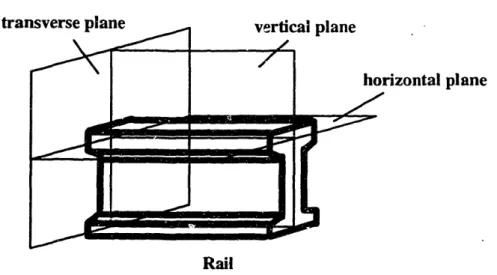
By definition, a transverse defect is any progressive fracture which occurs in the head of a rail and has a transverse separation [Sperry Rail Service, 1968]. Transverse defects (TD) include: 1) transverse fissures; 2) compound fissures; 3) detail fractures from shelling 4) detail fractures from head check; 5) engine burn and 6) welded burn fractures. A longitudinal defect occurs in the rail head that causes a longitudinal separation. Longitudinal defects include horizontal split heads (HSH) and vertical split heads (VSH). Figure 2.1 shows the positions of transverse and longitudinal planes for rail head.
transverse
nLane-rizontal plane
Rail
Figure 2.1: Transverse, Horizontal and Vertical Planes for Rail Head
A transverse defect starts from an internal imperfection in the steel, such as a shatter
crack. Impact of the wheels and bending stresses start the growth of a transverse
separation around the imperfection. A split head defect starts from an internal longitudinal seam, segregation, or inclusion. Growth is usually rapid, once the seam or segregation has opened up anywhere along its length. It continues until the split begins to turn outward [Sperry Rail Service, 1968]. Defective rails may be removed from track or protected by joint bars across defects [Hay, 1982].Rail fatigue failure is affected by operating conditions, maintenance activities, the contact area of rail and wheel, and material properties. The following is the summary of factors affecting rail fatigue:
1) maintenance practices:
grinding of rail head for the desired rail shape and the rem6val of surface defects; lubrication on rail for reducing friction between wheel and rail and.decreasing rail head wear.
2) traffic characteristics:
wheel load, annual traffic volume measured in million gross tons (MqT).
3) deterioration due to other distress conditions:
rail wear, deterioration levels of tie and ballast. 4) material characteristics:
rail size, rail strength, track stiffness. 5) track geometry:
curvature, alignment and gradient of track.
6) factors (other than curvature) affecting the contact area between wheel-and rail: speed, rail crown radius, wheel size, and wheel profile radius.
7) other location and environmental factors:
strength and drainage of soil and rocks, climate, etc.
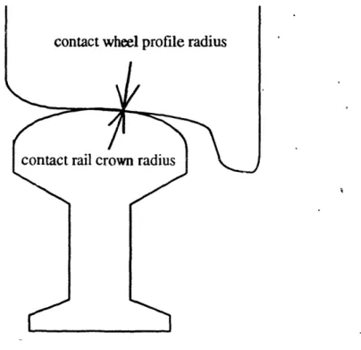
Measurement of most of the factors in the first five categories are often available in field data. However, the contact area derived from the contact rail crown radius and wheel profile radius, as shown in Figure 2.2, cannot be accurately measured from field
data because the contact point between wheel and rail changes with speed and curvature.
In addition, the environmental factors may be difficult to measure. As a result, these factors may become unobservable location specific errors in the field data. Data availability issues are discussed in great detail in Chapter 5.
contact wheel profile radius
Figure 2.2: Contact Rail Crown Radius and Wheel Profile Radius
Based on mechanical theories of rail fatigue and previous empirical studies conducted by the Association of American Railroads [1988] and by Abbott and Zarembski [1987], the fundamental relationships among fatigue failure rate (such as defects per mile per year) and some of the factors listed above are as follows:
Positive correlation: defect rate is expected to increase as the values of the, following variables increase.
- wheel load
- cumulative MGT
Negative correlation: defect rate is expected to decrease as the values the following variables increase.
- rail weight
- rail hardnessThere is no a priori expectation in regard to the relationships between fatigue failure and other explanatory variables such as lubrication, grinding, wear rate, speed, and curvature. The above relationships can be viewed as a priori expectations, to determine whether statistical estimation results are reliable and consistent with the current knowledge of rail fatigue behavior.
2.2 An Existing Engineering Model - The Phoenix Model
Mechanical theories and engineering analyses regarding rail fatigue behavior have been studied for some time. The engineering approach to rail fatigue analysis explores the mechanism of rail fatigue using mechanical theories and laboratory results based on material properties. Fowler [1976] and Journet [1983] developed theories of the mechanism of fatigue crack initiation and propagation. Ali [1992] applied fundamental fatigue theories to predict the fatigue life of railway bridges.
Another application of rail fatigue theories is the Phoenix model [Steele, 1990]. The Phoenix model adopted basic rail fatigue theories developed by Fowler [1976] and other related studies. This model was developed by the Association of American Railroads (AAR) to analyze fatigue behavior under various material properties, operating conditions, and maintenance practices. The following is a brief description of this model.
The Phoenix model simulates the mechanical processes leading to the initiation and growth of fatigue defects. That is, the Phoenix model first calculates the stresses within a rail head for given wheel loads, rail metallurgy, rail wear rate, foundation strength, wheel
size, and the contact rail crown radius and wheel profile radius. Then, by using the S/N curves (number of cycles to crack initiation for various stress levels, obtained rom laboratory experiments), the Phoenix model estimates the service exposure in million gross tons (MGT) until the accumulated stress is sufficient to produce the first manifestation of a fatigue crack beneath the running surface of the rail.
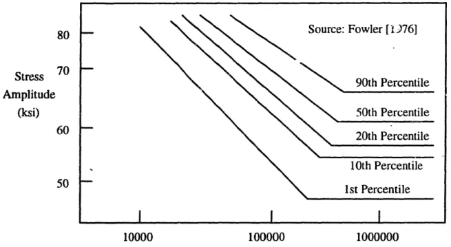
Because S/N curves may vary from one rail sample to another, Figure 2.3 shows the aggregate S/N curves based on the laboratory testing results from rail samples used in Fowler's study [1976]. Multiplying the number of loading by the stress level from Figure 2.3 produces estimated cumulative MGT for various rail failure rates. The Phoenix model uses the results from Figure 2.3 to estimate the cumulative service exposure for a crack to be initiated in terms of MGT at 1%, 5%, 10% and 20% sample failure rates.
80
Stress 70
Amplitude
(ksi)60
50 10000 100000 1000000Cycles to Crack Initiation (number of loadings)
Figure 2.3: Aggregate S/N Curves
I 1 I I
I
In other words, the Phoenix model predicts the cumulative MGT when a given percentage of rails begin to develop cracks the rail heads. Eventually, these cracks can
become fatigue defects. But, the Phoenix model is not able to predict defect type which
depends on the directions in which these cracks grow.However, the Phoenix model output appears to fall into two'different categories: one
category of data shows that the predicted fatigue life will be extended as wear rate
increases while the other category shows the opposite result. Based on the hypothesis that
TD would decrease while split head (SH) defects (i.e., VSH and HSH) would incease as wear rate increases, the defect types in the Phoenix model output can be implicitly revealed. The following is a detailed description of the hypothesis':TD is initiated at the point beneath rail head where the maximum stress occurs. As wear rate increases, the point with maximum stress will be moving downward. Since the point with maximum stress is not stationary, the damage due to the maximum stress is not accumulated at the same point. Therefore, the points where TD would have occurred will not develop TD if wear rate increases.
On the other hand, SH often occurs in the middle of rail head where significant tensile stress is formed. This tensile stress is not as significant as the maximum stress found in the point where TD-occur, thus, it is believed that a TD will initiate before a SH to occur. However, this tensile stress almost remains stationary as the wear loss of rail head increases. As a result, in case of increasing wear rate, the damage due to this tensile stress will be higher than the damage due to the maximum stresses. In other words, the chances
of having SH enhance as wear rate increases because the tensile stress formed in the middle of rail head become a dominate cause for a SH defect.
It should be noted that, at the stress levels at which crack initiation is calculated to
occur, the usage duration up to crack initiation accounts for 90 to 95 percent of the usage
duration up to forming a defect. Thus, the usage duration up to crack initiation isadequate for most engineering estimates.
In addition to the unknown defect types, there are a number of limitations to applying the current Phoenix model to rail fatigue analysis [Steele, 1988]. For instance, some input variables to the Phoenix model cannot be measured from field data; some fatigue mechanisms are still unknown at present; and some important factors are not included in the Phoenix model. Specifically, the limitations are:
1) Input variables that cannot be measured in the field.
As stated in Section 2.1 and shown in Figure 2.2, the contact rail crown radius and wheel profile radius cannot be measured in field data. Therefore, it is difficult to validate and to apply the Phoenix model using field data. The contact area should be a function of speed, curvature, wheel load, and rail and wheel shapes. A model to incorporate these variables has not yet been developed. As a result, the contact stress derived from the size of contact area and the amplitude of wheel load, cannot be accurately estimated when applying the Phoenix model for fatigue prediction.
In addition, the Phoenix model simulates rail wear as the removal of rail surface while maintaining the original shape of the rail head. However, the actual shape of the rail head after wear would not be same as the original due to uneven wear resulting from the dynamic contact path between rail and wheel.
The residual stress, caused by plastic deformation during the release of load, that built up within any rail is entirely unknown and cannot be predicted accurately at present from a knowledge of service history.
Moreover, the inherent fatigue resistance character of rail steel .can be highly variable and is unknown for any individual rail or group of rails. Small variations in stress state or material fatigue resistance may yield large variations in fatigue life. For this reason, the usage limit of fatigue failure is difficult to predict. An aggregate S/N curve is needed to explain this variability.
3) Missing or omitted variables
The Phoenix model is a tangent track model and thus cannot reflect the impact of curvature on rail fatigue.
The Phoenix model has been verified by limited data generated from the Facility for Accelerated Service Testing (FAST), a laboratory for railroad deterioration study. However, the model has not yet been validated by actual railroad defect data. The above limitations also underscore the reasons why results from the Phoenix model could be biased. Therefore, it is necessary to identify potential biases in the Phoenix model by incorporating field data.
A detailed discussion of the input variables and the output of the Phoenix model are
presented in Chapter 5.2.3 Current Statistical Approaches to Rail Fatigue Analysis
Most of the fatigue related studies apply theories of materials science rather than statistical methods to analyze the relationship among fatigue failure rate, usage duration,
[1992] combined field observations and Phoenix model output using a Bayesian procedure to predict fatigue defect rate. This method will be described in more detail in Chapter 3.
Since the studies of fatigue behavior are similar to the analyses of mortality and survival, i.e., the units with no defects can be viewed as surviving units while the defective units can be viewed as perished units, the methodology of survival analysis which is often applied in reliability studies, can also be applied to fatigue analysis.
The following are the general terminology used in survival and reliability analysis:
Definition:
X = a non-negative random variable representing the usage limit,
Fx (x) = P(X
<
x) = the cumulative distribution function (CDF) of X evaluated at x,
fx(x) = the probability density function (PDF) of X evaluated at x, Sx (x) = 1- Fx (x) = the survival function of X evaluated at x,
ho (x) = fx (x) / Sx (x) = the hazard function of X evaluated at x.
The hazard rate represents the force of mortality in the survival analysis because it refers to the death rate on surviving population. As for rail fatigue analysis, since a defective rail has to be replaced if detected, the hazard function represents the conditional probability of observing a failure in the surviving rails. The hazard rate can be interpreted as the deterioration rate and can be used as performance index for maintenance actions. For example, if the hazard rate is defined as having a fatigue failure, during year t given that the rail has no defect up to year t- 1, then multiplying the hazard rate by the number of rails in a segment produces the expected number of defects during year t. Therefore, if the expected number of defects per mile for a rail segment exceeds the allowable defect limit in any given year, then it is more economical to replace the whole segment than to
rail fatigue analysis is measured in cumulative million gross tons (MGT) of traffic. A detailed formulation of hazard rate is described in Chapter 4.
The basic relationships among hazard function, survival function, CDF, and PDF of any failure distribution are reviewed in Appendix A.
The focus of statistical fatigue analysis is to find the relationship between observed fatigue failure and usage, i.e., to search for the best fitted distribution among a group of
failure distributions.
Many failure distributions have been proposed for survival and reliability analysis. Appendix A lists most of the failure distributions used in the survival models developed by Elandt-Johnson and Johnson [1980]. One distribution is derived by Birnbaum and Saunders [1969]. This distribution was originally developed to model fatigue behavior. It assumes that each loading will result in a growth of crack, and the length of the growth is a normal distribution random variable. When the sum of crack growth exceeds a critical length, then fatigue failure will occur. 'The details of this distribution are shown in Appendix B.
The most commonly used distributions are the exponential distribution, the Weibull distribution, and the log-normal distribution. As shown in Appendix C, the exponential distribution assumes constant hazard rates. However, empirical study [AAR, 1988] shows that the hazard rate is not constant in rail fatigue. On the other hand, most of the other distributions used for survival analysis do not have closed forms for the hazard rate. As a result, the most commonly used distribution for rail fatigue analysis is the Weibull
distribution.
Compared to the exponential distribution, the hazard rate of the Weibull distribution will change over time. The Weibull distribution [Weibull, 1951] was first derived as a
model of failure of a mechanical device composed of several parts. This distribution is commonly used in the theory of reliability and biological researches. For example, the Rail Performance Model (RPM), was developed by Wells [1983] to predict defect rate using the Weibull distribution; a system of equations using the Weibull distribution calibrated to Phoenix model output [Shyr and Martland, 1990] had also been used as part of an simulation model called Total Right-of-way Analysis and Costing System (TRACS); Armitage and Doll [1954] and many others also developed models: for initiation of cancer using the Weibull distribution. The PDF and the CDF of Weibull distribution are as follows:
f(x)=
exp[-(x /
1)"
I
F(x) = 1- exp[-(x /
1)"
]
By definition, the survival function and the hazard function of Weibull distribution become:
S(x) = 1- F(x) = exp[-(x
/
1)
']
h(x) f(x)
h(x)=f(x)
= o
x"-'for a>O,
3>0,
x>O
There are two parameters in the Weibull distribution: a and 3. a is called the slope parameter and p is called the characteristic or scale parameter. If a > 1, the hazard rate increases as usage level x increases. If a = 1, then the Weibull distribution becomes the exponential distribution.
The AAR [1988] fitted a Weibull distribution to aggregated fatigue defect data from various railroads. Current practices in fitting failure distribution with aggregate defect records are based on the following assumptions: 1) defects occur randomly and are
MGT) needed for a defect to develop follows the Weibull distribution. The detailed procedures are described below:
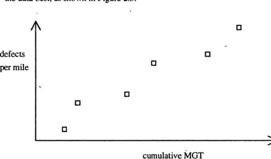
1) aggregation of defect records into a cumulative defect rate.
For defects occurring in segments with the same conditions, plot the cumulative
defects per mile with the corresponding cumulative MGT. Figure 2.4 shows the
result of this procedure.
2) conversion of the cumulative defect rate into percentage of rails failed.
The length of a rail is usually set to be 39 feet long, therefore there are 271 rails in one mile of track. Dividing the cumulative number of defects per mile by 271
produces the corresponding percent failure, i.e., F(x).
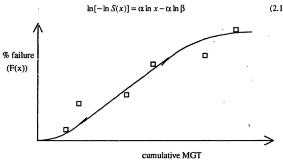
3) estimation of the Weibull distribution parameters a and
3.
The estimation is performed by finding the distribution parameters, a and , that fit the data best, as shown in Figure 2.5.
/
defects
per mile0
0
a
rE 03cumulative MGT
The distribution fitting in fact can be performed by using a linear regression with the following transformation of the Weibull distribution:
ln[-ln S(x)] = an x - xln 13
(2.1)
% failure
(F(x))
cumulative MGT
Figure 2.5: Distribution Fitting Against Cumulative MGT
This approach has three disadvantages: 1) the estimation is often based on low failure rates because of limited failed sample, as a result, the goodness of fit is very poor; 2) this approach did not explore the relationship between defect rate and the operation and maintenance activities, and hence the results cannot be used for the prediction of future deterioration conditions; and 3) this approach did not consider the different patterns for different types of failures.
Assuming that the different types of failures are independent, Elandt-Johnson and Johnson [1980, pp. 273] derived the overall hazard rate as the sum of hazard rates from all causes. A detailed of the formulation is also presented in Chapter 4.
A multiple failure model had been proposed by Moeschberger and David [1972] in life tests under competing risk causes. Their model assumes that two types of failures occur in two components. Further, the failures in component 1 and 2 leading to a system
failure are not independent. In other words, the failure of a system consists of three events: failure of component 1 alone; failure of component 2 alone; and failure of component 1 and 2 simultaneously. The model further assumes that the failure distribution follows exponential distribution with three constant hazard rates for each events. This model was also adapted by Manton et al. [1976] in studying the simultaneous
occurrence of various diseases.
Another model of multiple failures is proposed by Gilbert [1992] for a duration model of car ownership. This model consists of three independent events: replacement with a new vehicle; replacement with a used vehicle; and disposal without replacement. Gilbert's model also adapted the framework of hazard rate with multiple failures derived by Elandt-Johnson and Elandt-Johnson [1980], i.e., the overall hazard rate of ending the ownership of a vehicle is the sum of hazard rates from the above three causes.
The rail fatigue model presented in Chapter 4 is tformulated with the inclusion of multiple defect patterns based on an extension of the methodlogical framework derived by Elandt-Johnson and Johnson [1980].
Chapter 3: Review of Data Combination, Measurement Error and
Temporal Correlation Methods
3.1 Methods for Data Combination
The basic rational in data combination is the use of multiple data sources to construct a more reliable model when each type of data has a different level of accuracy and systematic bias. There are several methods used to combine different sources of data. The following is a brief description of the basic assumptions, the theoretical background, and the limitations of each technique.
3.1.1 Bayesian Updating Method
The Bayesian updating method consists of the prior distribution which represents the beliefs of the distribution of model parameters prior to the collection of any data, and the posterior distribution which represents the new beliefs about the distribution of model parameters conditional on new observed data [Lindgren, pp., 403-405, 1976].
Definition:
0 = model parameters,
z = the new collected data,
f(z I 0) = the distribution of z conditional on 0,
g(O) = the prior distribution of 0,
h(0 I z) = the posterior distribution of 0, such that
h(0z ) = f(zl0)g(0)
f(zlO)g(O)dO
In other words, the posterior distribution is the product of the prior distribution and the likelihood function of the observed data z.
If the prior distribution is a normal distribution that represents the distribution of 0 conditional on previous data, and the distribution of new data z is also a normal distribution, then, the posterior distribution conditional on new data z will become a normal distribution with means and variances equal to the updated model parameters and their variances. The Bayesian method in the single parameter case is described below.
Definition:
b,, a - the estimated parameter value and its variance from the previous data,
b2, ar = the estimated parameter value and its variance from the new data,
, ( = the updated values.
Then, the updated values are given by:
= b + (b, -b2)
(3.1)
= (a
2+
2)
112(3.2)
where,
a=
a2
/ (2+ o
) =weight for combining old and new estimates,
As shown in equation (3.1), the updated parameter is a linear combination of the parameters from the two data sources and the weight depends on the variances of model
parameter from both data sets. This method was proposed by Atherton and Ben-Akiva
[1976] for updating travel demand models.A similar approach had been applied by Campodonico [1992] for combining field data and Phoenix model outputs to predict rail fatigue failure. Because field data are often limited, Campodonico used Phoenix model output as a reference data source to build the prior distribution and then used the field data to obtain the posterior distribution.
F(x) = 1- exp[-(x /
3)"
]
where x is the usage of a rail measured in MGT and F(x) is the CDF of x. Therefore, the task of the calibration is to find the best fitted Weibull scale parameter 3 and slope parameter a for both field data and Phoenix model output. Unlike most of the applications of the Bayesian method that assume normal distribution for model parameters, this study assumes that the slope parameter a follows Gamma distribution while the scale parameter
[3
follows uniform distribution. However, the selection of these two distributions was not justified by Campodonico. The joint prior distribution was then specified as follows:(a, ) =f, (a)f
2(P)
(3.3)
where
f, = the Gamma density function,
f2 = the uniform density function.
As described in Chapter 2, the Phoenix model predicts the cumulative MGT at which 1%, 5%, 10%, and 20% rails failed due to fatigue for each input condition. The Phoenix model output were used to obtain values of a and 5 by running least square regression on the following transformed equation derived from the Weibull distribution:
ln[-ln S(x)] = aln x -aln
where S(x) is the survival function, i.e., l-F(x). Then the set of estimated a's and 3's were used to calibrate the parameters of the prior distribution.
Applying the Weibull distribution, the expected number of defects Mi occurred in a
M
i= L[F(xi)-F(xi,
)]
= L[-]-p(xi,
/
13)a]
-exp[
-(x
i/))"1]]
(3.4)
where
L = the number of rails in the segment,
xi = the cumulative MGT at the end of thej-th usage period.
Then, given L and the value of a and , Campodonico formulated the conditional probability of observing kj defects during this usage period as:
P(kiloa,P,L) = (Mj)
e
-M
%(3.5)
k !I
In other words, Campodonico assumes that the number of defects occurred in a rail segment follows a non-homogenous Poisson process, i.e., defects occur randomly across all locations within the same period of time, but the occurrence rate depends on the
duration of usage. Thus, the likelihood function of a and for observing the sequence of
defects becomes:(j)kj
(kl a, , L)=
-rIi
eM
(3.6)
j=l kji
where k = [
1,
k, ..., k,] and J is the number of usage periods.
Having obtained the likelihood function and the prior distribution, the posterior distribution then can be derived by Bayes Law as follows:
(cx, 13k, L) _
£(kla,P,L)i(a,)
(37)
J(kl a, , L)7(c, 13)dad
As a result, the probability of observing k defects during the j-th usage period
becomes:P(kjI L) =
J
P(k
I
,
,
L)(a,
k,L)dad
(3.8)
a13
The main disadvantages of Campodonico's approach for rail fatigue modeling are that
the updated model parameters do not take into account: 1) thebias in the Phoenix model output; 2) the different types of defects may have different parameters; an(' 3) the effects of operation and maintenance conditions on rail fatigue.A more general method of weighting parameters from multiple data sources, the combined transfer estimator, will be presented next.
3.1.2 Combined Transfer Estimator (CTE)
CTE is a minimum-mean-square-error estimator derived by Ben-Akiva and Bolduc [1987]. That is, although it is biased, the variance of the updated model parameters plus the square of the bias is less than the variance of the old model parameters. Using the same notation as in section 3.2.1 produces:
Var(b) + [E(b)-132]2 < Var(b2)
(3.9)
where p2 is the true parameter of the new data [pp. 2, Ben-Akiva and Bolduc, 1987]. In the single parameter case, the updated value and its variance become [pp. 4, Ben-Akiva and Bolduc, 1987]:
b
= b2+X(b -b
2)
(3.10)where,
=
a
2 / D = weight for combining b: andb
2,D
= (+ 2+ A2)
A = b - b2 = an estimate of the bias in b.
CTE is an extension of the Bayesian updating procedure because it explicitly accounts for the presence of a transfer bias, i.e., the bias in b. Compared to the Bayesian updating method, this method gives more weight to the parameters from new data (b2 ).
This method also suggests a range of transfer bias where the previous data set could be used for combined estimation. That is, if the model estimated from the old data is not significantly different from that estimated from the new data, then CTE could be used to obtain the updated parameters; otherwise, using the old model parameters is not justified.
In conclusion, the advantage of the CTE is that the updated model parameters can be directly calculated from the estimated parameters and their variances from two data sources. This precludes the need for pooling data sources and re-estimating the model
parameters. Furthermore, CTE is shown to be more accurate in terms of the mean square
error than a direct non-transfer estimator (i.e., 2 by itself).3.1.3 Joint Estimation
Recent studies on RP and SP data combination were conducted by Morikawa [1989] and Vieira [1992]. Both studies applied data combination methods to discrete choice models. The following is a brief description of the joint estimation method for the data combination of field data and laboratory data in deterioration modeling:
Define