HAL Id: hal-02307246
https://hal.archives-ouvertes.fr/hal-02307246
Submitted on 7 Oct 2019
HAL is a multi-disciplinary open access archive for the deposit and dissemination of sci-entific research documents, whether they are pub-lished or not. The documents may come from teaching and research institutions in France or abroad, or from public or private research centers.
L’archive ouverte pluridisciplinaire HAL, est destinée au dépôt et à la diffusion de documents scientifiques de niveau recherche, publiés ou non, émanant des établissements d’enseignement et de recherche français ou étrangers, des laboratoires publics ou privés.
On equivalent hydraulic conductivity for oscillation–free
solutions of Richard’s equation
Benjamin Belfort, Anis Younes, Marwan Fahs, François Lehmann
To cite this version:
Benjamin Belfort, Anis Younes, Marwan Fahs, François Lehmann. On equivalent hydraulic conduc-tivity for oscillation–free solutions of Richard’s equation. Journal of Hydrology, Elsevier, 2013, 505, pp.202-217. �10.1016/j.jhydrol.2013.09.047�. �hal-02307246�
On equivalent hydraulic conductivity for oscillation–free
solutions of Richard’s equation
Benjamin BELFORT*, Anis YOUNES, Marwan FAHS and François LEHMANN
Laboratoire d’Hydrologie et de Géochimie de Strasbourg, Université de Strasbourg - CNRS/UMR 7517
1 rue Blessig, F- 67084 Strasbourg, France.
Submitted to Journal of Hydrology
Recieved: 04/24/2013 – return to authors: 06/13/2013 Revised manuscript send: 12/09/2013
* Corresponding author
Laboratoire d’Hydrologie et de Géochimie de Strasbourg Université de Strasbourg - CNRS - UMR 7517
1 rue Blessig, 67084 Strasbourg, France Tél : 33 368 850 386
Fax : 33 368 850 402 Mail : [email protected]
Abstract
The estimation of numerical equivalent conductivity remains a crucial issue for the accuracy and stability of the solution of the nonlinear Richards’ equation (RE) when modeling variably saturated flow. In the literature, it appears that this topic has been typically considered for one-dimensional discretization despite the growing interest in multidimensional problems. After reviewing different possibilities of equivalent hydraulic conductivity estimation, we evaluate their ability to yield monotonic results. Hence, the monotonicity analysis provided by Forsyth and Kropinski (1997) has been generalized for the different equivalent conductivity formulations. On one hand, the upstream mean is unconditionally stable but is also known to overestimate the conductivity. On the other hand, other formulations, including Darcian mean approximations, can be accurate and straightforward to adapt in multidimensional codes but do not always provide monotonic solutions of the RE. An adaptive algorithm is presented, which adapts the conductivity in function of the monotonicity condition, i.e., a variable criterion based on the conductivity at nodal points, the conductivity averaging technique and the piezometric head variation. The proposed numerical method can be implemented in existing multidimensional codes. Numerical investigations in steady state and time-varying conditions, 1D and 2D cases, and homogeneous and heterogeneous media confirm the interest in the proposed algorithm.
Key words: numerical methods, unsaturated flow, Richards’ equation, internodal conductivity, mass-lumping, monotonicity.
1. Introduction
Modeling water flow in variably saturated soils is of great interest to many scientific research and engineering applications involved in the management of water resources. Richards’ Equation (1931) (RE) has been described as a valuable model to predict water movement in variably saturated media and to provide inputs for contaminant transport models (Šimůnek and Bradford, 2008). The development of robust and fast numerical simulators for unsaturated flow remains a challenging research subject of research (Crevoisier et al., 2009; Kuráž et al., 2010; Wu, 2010; An et al., 2011; Zadeh, 2011, Lott et al., 2012; Zambra et al., 2012). In fact, when simulating unsaturated flow in porous media, numerical oscillations may occur when the spatial distribution or temporal evolution of the pressure head or water content fluctuate around the correct value. Traditionally, the issue of oscillation is typically raised for methods based on variational formulation, such as finite element (FE) (Neuman, 1972; Sandhu et al., 1977; Vermeer and Verruijt, 1981; Milly, 1985; Celia et al., 1990; Pan et al., 1996; Wood, 1996; Thomas and Zhou, 1997; Karthikeyan at al., 2001). Many studies dealing with RE focus on the numerical expression of the mass matrix for time-dependent problems and conclude that the diagonalized (or lumped) form is preferred to avoid oscillations (Neuman, 1972; Cooley, 1983; Milly, 1985; Celia et al., 1990; Pan et al., 1996; Ju and Kung, 1997). In this context, the M-matrix property (i.e., a non-singular matrix with positive diagonal and negative off-diagonal coefficients) is often used to establish conditions that ensure consideration of the maximum principle (Windisch, 1989; Wood, 1996; Thomas, 1997; Hoteit, 2002; Belfort and Lehmann, 2005; Younes et al., 2006). This suitable mathematical property prevents unrealistic results in the case of saturated flow but is not sufficient for unsaturated flow (e.g., Forsyth and Kropinski, 1997).
However, the behavior of the solution is dependent on the equivalent conductivity (Keq) used in the numerical method for the spatial discretization of RE. Keq represents the
mean value of the hydraulic conductivity related to Darcy–Buckingham’s law and is calculated between two cells or control volumes for finite difference (FD) and finite volume (FV) methods (Haverkamp and Vauclin, 1979; Schnabel and Richie, 1984; Warrick, 1991; Zaidel and Russo, 1992; Baker, 1995; Romano et al., 1998; Gastó et al., 2002; Brunone et al., 2003), or inside the element for finite element (FE) and mixed hybrid finite element (MHFE) methods (Farthing et al., 2003; Belfort and Lehmann, 2005). Previous studies consider the relation between a formulation of equivalent conductivity and the accuracy of the numerical solution. In fact, studies have been found whose authors recommended the use of the geometric mean (e.g., Haverkamp and Vauclin, 1979), arithmetic mean (van Dam and Feddes, 2000), harmonic mean (Oldenburg and Pruess, 1993), upstream mean (Oldenburg and Pruess, 1993), integrated mean (Pei et al., 2012), or more complex averages, such as the Darcian mean (Warrick, 1991; Baker et al., 1995) or optimized algorithm (Szymkiewicz, 2009). A review on averaging approaches for the computation of inter-nodal permeabilities is given in the chapter 4 of the book by Szymkiewicz (2013). Based on many studies on the subject, it appears that a single simple average could never be adapted for the various combinations of soil materials, spatial grid sizes and water flow conditions. Additionally, the difficulty in incorporating soil heterogeneity in the estimation of the hydraulic conductivity has been studied, typically for the one-dimensional FD method (e.g., Romano et al., 1998; Szymkiewicz and Helmig, 2011).
Only a few authors consider the Keq selection to avoid oscillations (Baker et al., 1999; Forsyth and Kropinski, 1997; van Dam and Feddes, 2000; Baker, 2006; Szymkiewicz, 2009). Among the different methods, it has been shown that the Darcian mean approximations produce accurate results (Warrick, 1991; Baker, 2006; Szymkiewicz, 2009). However, Darcian mean approximations generally require numerical efforts to be implemented into existing codes, cannot always accept specific relationships describing retention and
conductivity and their extension to multidimensional cases with complex geometries remains a challenging issue.
This study focuses on the numerical solution of water flow problems described by the standard RE, i.e., rigid porous media are considered and infinite air phase mobility is assumed. Because monotonicity constitutes the central issue of the paper, other significant research areas, such as linearization strategy (Lott et al., 2012), non-equilibrium and dynamic effect (Schweizer, 2012) are not investigated. Nonetheless, it should be noted that the results obtained in the current study could be applied to a large variety of numerical codes dealing with variably saturated flow problems.
The main objectives of this study are as follows: 1) review the different estimations of equivalent conductivity, 2) analyze their ability to yield monotonic results from a mathematical viewpoint, 3) test a new switching algorithm for a multidimensional implementation and 4) study the efficiency of the different averaging techniques by considering several 1D and 2D test cases.
2. Unsaturated flow modeling
The mathematical model used to describe the physical problem of water flow in unsaturated soil is given by the combination of Eq. [1] and Eq. [2]. Darcy–Buckingham’s law defines the water flux in the domain as follows:
h . H q K [1]
where q is the macroscopic fluid flux density [L.T-1]; K is the hydraulic conductivity [L.T-1]; and H [L] and h [L] are the piezometric and pressure head, respectively, such that H h z, where z is the depth with upward being positive [L]. The mass conservation of water, under the assumption of incompressible media and fluid, leads to the mixed form of RE as follows:
. f t
q [2]
where θ is the volumetric water content [L3
.L-3]; t is the time [T]; f is a source/sink term [T-1]; and q is the previously defined water flux.
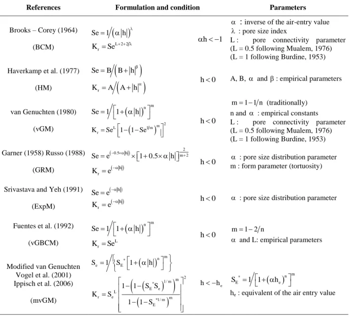
To solve the governing flow equations, initial and boundary conditions should be specified. Moreover, the interdependencies of h, θ and K should be characterized using constitutive relations (often exponential or power functions). Table 1 summarizes different relative conductivity functions, such as K h
KsK hr
, and the referred effective saturation (Se) [-] is defined by rs r
Se
. Ks is the saturated conductivity [L.T
-1
], which in
general may be a tensor, and s [L3.L-3] and r [L3.L-3] are the saturated and residual
volumetric water contents, respectively.
As reported in literature and depending on the problem considered, specific storage coefficients can be included in the RE to account for fluid compressibility and solid matrix
pressure head as the main variable, requiring specific attention when expressing the capillary capacity (Celia et al., 1990; Rathfelder and Abriola, 1994). Because the main objective of this study is not dependent upon the precise form of the RE, only the mixed form (Eq. [2]) will be considered.
3. Numerical resolution of Richards’ Equation
3.1. Presentation of numerical methods
When numerical methods are used to solve a physical problem modeled by the RE, the differential equation is integrated over the solution domain Ω, which is decomposed into a set of non-overlapping smaller subdomains Ωe (such as e). The unknown variables and dependent coefficient are generally approximated at nodal points for FE or at the center of each control volume for FD and FV. The MHFE method uses both cell, and nodal (1D) / edge (2D) or face (3D) averaged values. Regardless of the method chosen, the final matrix system has the form:
x
x xA . H B . F 0
[3]
where x is a node (FE), cell (FD, FV) or face / edge (lumped MHFE) indice. Matrices [A] and [B] consist of the spatial and temporal approximations obtained from the numerical approximation on each subdomain,
ee
A
A and
ee
B
B , respectively. It should be noted that {F} contains sink / source terms and boundary conditions. The ith ordinary differential equation, referred to as gi, is:
i i n 1 n n 1 n n 1 n 1 n 1 i i i j j ij j i j i, j n 1 n n 1 ij j j i n 1 j g H , H , H , H A H H 1 + B F 0 t
[4]where ηi includes node i and the set of its neighboring nodes; and σi represents the (set of) element(s) sharing node i. The expressions for matrices [Aij] and [Bij] for different formulations of FE and MHFE methods can be found in literature (e.g., Huyakorn et al., 1984; Chavent and Roberts, 1991; Belfort et al., 2009). It should be noted that for the FD / FV methods, the previous matrices are given by Eq. [5] and Eq. [6]:
ij s r,ij ij
A K .K . [5]
where Kr,ij is the conductivity between cells i and j; and γij refers to the interface area between i and j divided by the distance between them.
e
ij e ij
B V [6]
where Ve is the length (1D) / surface (2D) / volume (3D) of element ―e‖; and δij is the Kronecker operator. The previous definition must be modified in the case of non-orthogonal control volumes (Loudyi et al., 2007).
3.2. Monotonicity conditions
The monotonicity analysis is typically performed by considering the general form of the discretized RE (Eq.[4]). Following Forsyth and Kropinski (1997), it is established that a monotone discretization does not contain any local minima or maxima for all its interior homogeneous nodes:
min n 1 max
i i i
H H H [7]
The monotonicity analysis can be achieved on the discretized (but not linearized) system of equations [4], which is equivalent to the opposing expression of Forsyth and Kropinski (1997). According to these authors, a monotone solution is required to satisfy the following conditions for all interior nodes:
i
i
i n n 1 n 1 i j i g g g a 0 and b 0 and c 0 H H H [8]The different derivatives are given as follows:
n i i ii n n 1 n i i g 1 B H t H [9]
i n 1 n 1 j n 1 n 1 n 1 i i i ij ij n 1 n 1 n 1 n 1 j i, j j j g A 1 H H A + B H H t H
[10]
i i n 1 n 1 n 1 ij n 1 n 1 n 1 i i i j i ij ii n 1 n 1 n 1 n 1 n 1 j i, j i i i i n 1 n 1 n 1 ij n 1 n 1 n 1 i i j i ii ii n 1 n 1 n 1 n 1 j i, j i i i A g 1 F H H A + B H H t H H A 1 F H H A + B H t H H
[11]3.3. Analysis of methods to ensure monotonicity
3.3.1. The issue of equivalent conductivity to avoid unphysical oscillations
Despite the fact that FV and FD schemes satisfy the M-Matrix property by definition (Forsyth and Kropinski, 1997), it was shown that FD numerical solutions might exhibit unphysical oscillations (Forsyth and Kropinski, 1997; Baker, 2006, Szymkiewicz, 2009). Furthermore, in the case of unsaturated flow and condition b) of Eq. [8], the derivatives of the matrix [A] have to be considered, yielding a condition dependent on the estimation of the conductivity.
Interblock conductivity can be achieved using arithmetic, harmonic, geometric or more complex means of the hydraulic conductivities at the two adjacent cells (Haverkamp and Vauclin, 1979; Schnabel and Richie, 1984; Zaidel and Russo, 1992; Forsyth and Kropinski, 1995; Romano et al., 1998; van Dam and Feddes, 2000; Gastó et al., 2002; Brunone et al., 2003). Table 2 summarizes the main formulations of equivalent / interblock conductivity that have been studied particularly for 1D flow problems. For the weighted mean
proposed by Gastò et al. (2002) a critical size ( z . a
10a log N11
1) should be considered to avoid negative values of the conductivity, as is reported, for instance, by Szymkiewicz (2009) for large internodal spaces. Additionally, it should be observed that this weighted mean can be applied only for the van Genuchten (1980) and Brooks – Corey (1964) hydraulic models. Darcian mean approximations are preferred to avoid unphysical oscillations (Warrick, 1991; Baker, 1995; Baker et al., 1999; Baker, 2000; Baker, 2006). Table 3 provides the main formulas to compute the Darcian integral mean for the different hydraulic models. An adaptation is proposed to handle the classical formulation of the van Genuchten model rather than the simplified form used by Baker (2000). The weighting coefficients wGASTO (Gastó et al., 2002) and λDARC (see Table 3) are functions of the conductivity at the two neighboring nodes. Notice that their expressions are not symmetric. In addition, previous studies (Baker et al., 1999; Baker, 2000, 2006) have shown interest in changing the expression of the equivalent conductivity (referred in Table 2 as Koptim) in function of the ratio Δh / Δz. Due to the complex computation of Kdarcy, an alternative optimized algorithm has been recently developed to avoid oscillations (Szymkiewicz, 2009). The algorithm has been reproduced and slightly adapted to take into account the orientation of the vertical axis (see Appendice).The purpose of the following paragraph is to complete the analysis proposed by Forsyth and Kropinski (1997), which showed that the centroidal approximation is
conditionally stable and suggests the use of upstream mean. For FD / FV methods and FE and MHFE variational formulations based on a single point quadrature rule, the relative hydraulic conductivity between nodes i and j, noted Kr,eq, should be estimated according to the possible expressions of Table 2. Hence, the expressions are obtained as follows:
n 1 r,eq n 1 n 1 n 1 j i ij s j i ij ij n 1 n 1 n 1 n 1 j j j K g 1 K H H A + B H h t H [12]
i n 1 r,eq n 1 n 1 n 1 i i ij s j i ij ii n 1 n 1 n 1 n 1 j i, j i i i K g 1 K H H A + B H h t H
[13]According to Eqs. [12] and [13], the results of the monotonicity analysis may depend on the relative conductivity estimation. Table 4 contains the analytical developments of the spatial terms of Eq. [12] for different equivalent conductivity estimations, and Table 5 summarizes the results related to Eq. [13]. Regardless of the model chosen in Table 1 to describe the relationships between the pressure head and the relative conductivity, Kr(h) is an increasing function; therefore, the sign of its derivative remains positive. The sign of the expressions depicted in Tables 4 and 5 is important to determine if conditions b) and c) of Eq. [8] are satisfied. On one hand, we remark that the M-matrix criterion applied for the parameter γij is a necessary but not always sufficient condition. On the other hand, the monotonicity of the different formulations should be studied specifically as follows:
The analytical expressions corresponding to the arithmetic, geometric, harmonic and weighted formulations show that the monotonicity depends on the piezometric variation between adjacent nodes weighted by a coefficient dependent on the relative conductivity and its derivative. A criterion that may guarantee the solution’s monotonicity in the general case cannot be proposed.
For the upstream mean, if the M-matrix criterion is satisfied, conditions b) and c) of Eq. [8] are automatically fulfilled, as can be seen in Tables 4 and 5. Despite this interesting
property, the upstream formulation is sometimes avoided because of its overestimation of infiltration front.
Assuming that the M-matrix criterion is satisfied and considering the expressions provided in Tables 4 and 5 for the integral mean, one can deduce that monotonicity is always accounted for horizontal flow processes. This fact corroborates the experimental conclusion of Pei et al. (2012). For vertical discretizations, a limitation has to be added.
When the pressure gradient increases, i.e., the term ji
ji
h z
, Tables 4 and 5 show that
the monotonicity conditions are reduced to the M-matrix condition. However, when the pressure gradient decreases, monotonicity difficulties appear to satisfy condition c) of Eq.
[8] if ji ji h 0 z and condition b) if ji ji h 0 z
. It should be noted that the expressions of
Tables 4 and 5 could be modified if the z axis is not collinear to the gravity force by an angle φ. In this case, conditions b) and c) of Eq. [8] can be written as follows:
jir,int r,i r,i
ji z K K K 0 h [14]
ji r, j r,int r, j ji z K K K 0 h [15]with χ = cos(φ). Because Kr,int is between Kr,i and Kr,j, when h z
, Eqs. [14] and [15] lead to conditions [16] that can never be satisfied and are given as follows:
r,int r,i r,int r, j
K 2K and K 2K [16]
Hence, our mathematical analysis demonstrates that the integral formulation could produce unphysical oscillations. The analysis corroborates previous studies of the flux approximation based on a simple three-point grid (Baker, 2000, 2006; Szymkiewicz,
The monotonicity of the optimized algorithm (Szymkiewicz, 2009) is more difficult to attest. Hence, we provide in appendix an analytical analysis of monotonicity based on Eq. [8]. The main result is that the formulation used to estimate internodal conductivity during infiltration is unconditionnaly stable. For drainage, monotonicity has been demonstrated for the expression K1 based on the upper conductivity (see Eq.[A.2] in Appendix). The heuristic formulation used for K2 is conditionnaly monotonic. It should be noticed that the presence of relative conductivity derivatives in the final expressions prevents any general conclusions. Nonetheless, as stated by Szymkiewicz (2009), oscillations in drainage problem are linked with overestimation of internodal conductivity. Since the minimum value of (K1, K2) is chosen, monotonicity should be preserve. The complex heuristic formulation of Keq used for capillary rise does not allow us to conclude easily on monotonicity accordingly to the criterion of Eq. [8].
3.3.2. Propositions of algorithm
To simplify the presentation, we suppose that the multidimensional existing code uses a centroidal approximation for the evaluation of the equivalent conductivity. Centroidal approximation signifies that the conductivity over each element is computed from a combination of the conductivities at the nodal points (edges / faces). The arithmetic mean (e.g., Šimůnek et al., 2006) appears as a particular and, nonetheless, currently used technique. Hence, Eq. [10] is modified to hold this specific context:
ij ij i n 1 r,eq E n 1 n 1 n 1 i s i i ij s r,eq n 1 n 1 E i, j j K g K H H K K H h
[17]where Eij refers to the element containing nodes i and j;
ij n 1 r,eq E
K is the average conductivity over this element, and ηi includes node i and the set of its neighboring nodes. To obtain a
monotonic solution of the RE, we investigate two strategies presented in the following paragraphs.
For all the interior and homogeneous nodes of the domain, the monotonicity of the solution is tested at each time step.
With the first strategy (MS1), a subroutine tests the monotonicity of the solution at each time step. When unphysical oscillations are encountered, MS1 consists of stopping the iterative process, imposing the upstream formulation (either at specific nodes or at all nodes) and running the numerical code again for the problematic time step. Then, the equivalent conductivity retrieves its original formulation until oscillations reappear. The MS1 algorithm only considers the elements without sink / source term and whose neighbors are constituted of the same soil material.
In the second approach (MS2), the value of the equivalent conductivity is adapted in function of condition b) of Eq. [8]. Therefore, the algorithm is based on the following test:
ij
ij E i n 1,k r,eq E E n 1,k n 1,k n 1,k i ij s r,eq E s n 1,k i i i, j K i and j ,i j K K K H H 0 h
[18]where Ei refers to node i and the set of its neighboring nodes belonging to element E. During
the iterative process, either the equivalent conductivity satisfies Eq. [18] or the upstream approximation, which guaranties the monotonicity, is substituted. In fact, for a NE nodes element, Eq. [18] represents a system of NE
NE1
equations. It should be noted that the coefficients γij depend only on the mesh geometry and have been already computed for solving the matrix system corresponding to Eq. [3]. Only the derivative of Kn 1r ,eq
, i.e., especially the derivative of the K(h) function, could necessitate additional work. When the Newton-Raphson iteration is used, a subroutine is typically implemented for the analytical evaluation of these derivatives, which is required for the Jacobian matrix computation.
It should be noted that for different simulations, numerical codes based on the mass-lumped MHFE method have been used.
4. Numerical simulations
The purpose of this section is to illustrate the theoretical monotonicity assessments by computing the expressions of Table 4 for different types of soil, mesh sizes and constitutive relationships and investigate unsteady flow simulations showing the effect of the equivalent conductivity and efficiency of the proposed algorithm. The relative conductivity, water content and capillary capacity are computed directly from the definitions provided in Table 1. For the hydraulic models of van Genuchten (1980), Haverkamp et al. (1977) and Fuentes et al. (1992), the integral formulation of the equivalent conductivity is estimated with a Legendre numerical integration, whereas for the Brooks – Corey and the exponential models, the analytical expressions have been implemented. In addition, the derivatives in Table 4 are determined analytically, except for the derivatives of the weighting coefficient occurring in the weighted (wGASTO) and Darcian integral means (λDARC), which are estimated with a perturbation method. For the weighted formulation of Gastó et al. (2002), when the mesh size increases, the weighting coefficient can be negative. In this case, the upstream mean can substituted to avoid numerical problems.
4.1. Accuracy assessment for steady state flow
In this section, the expressions of Table 4 are computed without considering the coefficient γij, which depends on the numerical scheme and mesh geometry. Due to the
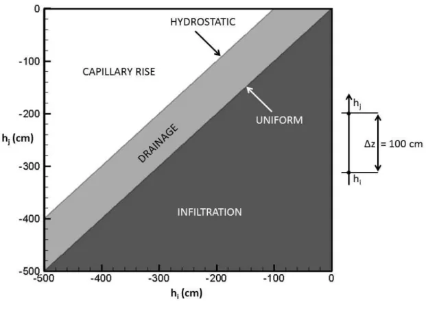
summation term and presence of mass variation for diagonal coefficients (see Eq. [13]), the expressions depicted in Table 5 are not computed. Sixteen types of soils covering different texture classes presented by Szymkiewicz (2009) have been selected. Five hydraulic models depicted in Table 1 are used and the corresponding parameters are reported in Table 6. We consider 25 x 104 possible values for the pressure variation (hj – hi), and the nodal distance dij takes the values of ± 1 cm, ± 10 cm, ± 100 cm or ± 200 cm along the vertical direction. As shown in Fig. 1, our numerical approach allows testing the monotonicity of the different equivalent conductivity formulations for various scenarios corresponding to infiltration, drainage or capillary rise. The behavior of the different means has been largely described in literature (Szymkiewicz, 2009) by comparing the accuracy of each formulation when the nodal spacing increases.
The results of these numerous simulations for vertical flow are summarized in Fig. 2. For each type of soil and nodal distance, we report the percentage of positive value for the coefficients of Eq. [12]. As expected, the upstream mean always leads to positive values for the coefficient of Eq. [12], and consequently, its results are not shown on Fig. 2. Below a critical mesh size, the weighted formulation of Gastò et al. (2002) has an approximately monotonic behavior. The geometric, harmonic and integrated means appear to be extremely sensitive to oscillation problems, especially for large grid size and coarse-textured soils. The Darcian integral mean is more interesting from this point of view. Contrary to the arithmetic mean, it remains stable when the mesh size increases. Finally, it is worth noting that Szymkiewicz’s algorithm produces montonic solution for the different grid sizes and soils used for these steady state cases.
4.2. Numerical simulations of time varying unsaturated flow
In the current section, we propose to analyze the efficiency of our monotonicity analysis by different test cases illustrating infiltration, drainage and evaporation processes for both one and two-dimensional problems. Both temporal and spatial unphysical oscillations are considered. For one-dimensional problems, a FD numerical code using the Thomas algorithm has been used to solve the mixed form of RE. The time step size management is achieved by using a heuristic method based on the number of iterations (Šimůnek et al., 2006). It should be noted that more advanced time integration methods (e.g., Miller et al., 1998) and/or time stepping techniques (Belfort et al., 2007) could be used to improve the efficiency of the model.
Besides, in this section, only some averaging techniques were selected either because of the performance obtained in the previous steady-state investigations and/or reported in literature (Kszym) or because of their adaptability in multidimensionnels codes (Karit, Kgeom). Hence, Kgasto, Kint and Kdarcy were not considered.
Statistical results are provided in Table 7 to illustrate the monotonicity and efficiency of various averaging schemes and algorithms for 1D problems. Hence, the root mean square
error,
z N 2 z i ref ,i i 1 z 1 RMSE N
, the potential head gradient and, the maximum pressure overshoot for infiltration have been reported. Fine grid solutions (Δz between 1 and 0.5 mm) have been computed and serve as reference solutions (Ɵref) for error calculations. For two-dimensional problems, the new algorithm has been implemented in a lumped MHFE numerical code. The linear system is solved with the preconditioned conjugate gradient method, and the time step size is heuristically adapted.4.2.1. Test problem 1: infiltration with constant head boundary condition in a 1D domain
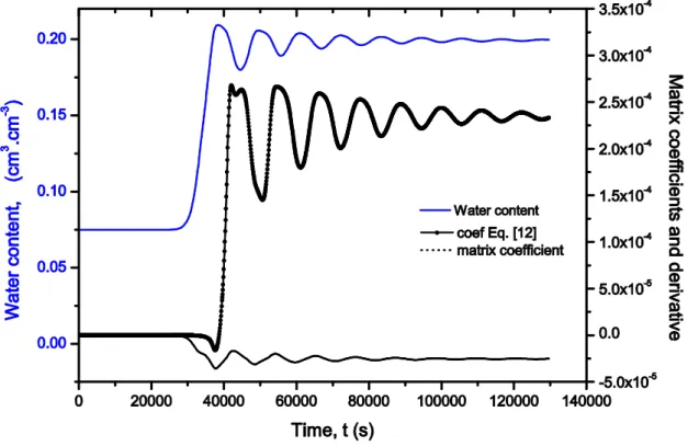
The first test case is selected from Baker et al. (1999) and demonstrates the difficulties of arithmetic formulation to produce physically admissible results. This case deals with infiltration in a 45-m-deep column, which contains moderately to coarsely textured soils. The soil hydraulic properties are characterized by Haverkamp’s model (see Table 1), and the parameters are summarized in Table 6 (soil n = °13). The media is initially dry, and h(z,0) = hinit = -929.8 cm. This pressure head is maintained at the bottom during the simulation, h(z = 450 cm, t) = hdown = - 929.8 cm, and the top boundary condition is h(z = 0 cm, t) = htop = - 20.7 cm. For the time step management, we adopt a minimum value of 10-3 s and maximum time step of 100 s. The simulation is performed over 1.5 days.
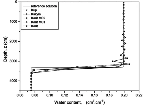
Fig. 3 describes the evolution of the water content at the position z = 1200 cm for a uniform mesh size of 150 cm. During the infiltration process, this type of profile should be monotone; however, large oscillations are observed in Fig. 3. The temporal evolution of the matrix coefficient corresponding to the modified Picard iteration method and the coefficient of Eq. [12] are also presented in Fig. 3. When the oscillations occur, only the coefficient of Eq. [12] becomes positive. This result demonstrates the necessity to include the derivatives in the monotonicity analysis. Comparisons between the standard approach and MS1 or MS2 algorithms are shown in Fig. 4, which depicts the profiles of water content after 30 hours of infiltration. On one hand, the arithmetic formulation exhibits large spatial oscillations when the grid size increases from 10 cm to 150 cm (Table 7), whereas the upstream approximation leads to an oscillation-free solution corresponding to a faster than expected wetting front. On the other hand, the Darcian mean approximation Kszym and the new algorithms associated with the arithmetic or geometric means produce physically admissible results. Statistical results presented in Table 7 show that many extremum appear with a standard approach based on
Kgeom or Karit. These failures correspond mainly to pressure overshoots that have been reported in Table 7 for different grid sizes. Indeed we provide the maximum value of the potential head gradient (referred as max
h
z
in Table 7); for a problem of infiltration, positive values indicate the presence of oscillation in the solution. On the contrary, Kszym and Kup do not produce any oscillations and have not been combined with MS1 or MS2 algorithms. We can observe in Table 7 that Kszym improves the accuracy of the solution obtained with the upstream mean. Otherwise, the MS2 algorithm detects many violations of the monotonicity criterion that lead to a conductivity modification. The MS1 algorithm avoids both the presence of oscillation in the solution and its propagation in the profile. Stabilizing the solution at a given time is necessary but not sufficient, and MS1 has to correct the conductivity regularly during simulation. For this first test case of infiltration in dry soil, the new algorithms maintain the precision of the results achieved by the arithmetic formulation and avoid spurious oscillations as depicted in Table 7 and Fig. 4. The precision of the new algorithm (MS1) is slightly better that the optimized algorithm (Kszym), mainly with the geometric mean.
Notice that the Newton-Raphson iterative method (Lehmann and Ackerer, 1998) and the Method of Lines (Miller et al., 1998) have been implemented and tested (results not shown). Even if these methods improve the convergence and rapidity of the computation, we can observe similar unphysical oscillations in the solutions.
4.2.2. Test problem 2: drainage in 1D sand column
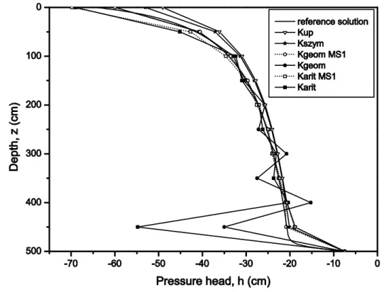
The second test problem, which has been investigated by Szymkiewicz (2009), studies the effects of other flow conditions. A 5-m-deep sand column (soil n = °5) is considered with the following properties: the media is quasi-saturated with a uniform pressure head distribution, h(z,0) = hinit = -7.5 cm, the lower boundary pressure head remains at the same
initial value while an impermeable boundary condition is imposed at the top of the column, and q(z = 0 cm, t) = qtop = 0 cm.s-1. The time step size varies automatically between 3.6 x 10 -6
s and 360 s according to the number of iterations. The pressure head profiles after 30 hours of drainage are illustrated in Fig. 5 which are similar to those presented by Szymkiewicz (2009). The simple averaging methods, Kgeom and Karit, produce large oscillations in the solution. The methods based on the Darcian mean produce oscillation-free solutions. The MS1 algorithm allows removal of the unphysical oscillations from the solutions obtained with the simple averaging techniques and conserves the trend of the chosen equivalent conductivity. Hence, the accuracy of the algorithm is good and for coarse grid slightly better than simple original formulations. As observed in Table 7, the monotonicity test is so restrictive that the MS2 approach uses many changes of the conductivity. Hence, the corresponding solutions are similar to Kup and have not been drawn. The monotonicity failures reported in Table 7 correspond to oscillations in the profile at a given time. Contrary to the first test case, these numerical artifacts do not produce overshoot of the maximum pressure head but the minimum value of the potential head gradient (referred as min
h
z
in Table 7) should be positive or null. Postive values of this gradient observed for Karit and Kgeom indicate spurious oscillations in the drainage process.
4.2.3. Test problem 3: intensive rain at a 1D dry heterogeneous soil
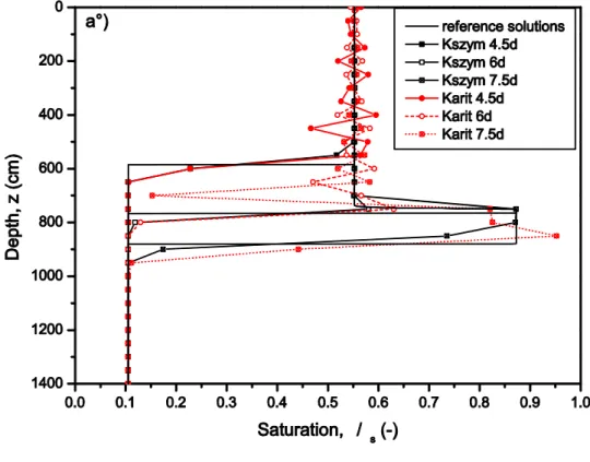
This test case allows investigation of the behavior of the averaged conductivity in the presence of soil heterogeneities. Two equal adjacent zones are considered, which represent a 14-m-deep one-dimensional domain. A rainfall rate of 0.25 m/day is applied over 7.5 days to an initially dry porous media (hinit = -1000 cm). The material properties correspond to a soil value of n = °1 in Table 6, except that the modified van Genuchten model is used with an air entry pressure of 2 cm. A simple heterogeneity has been generated by considering a saturated
permeability of the lower zone that is 10 times less than the original prescribed value in Table 6. The time step can vary between 1 x 10⁻⁶ s and 100 s according to a heuristic management. In this test case, spurious oscillations occurring upstream of the permeability discontinuity are reported in a few profiles of saturation (Fig. 6). From a physical point of view, the relatively small contrast of permeability causes a natural increase in saturation in the middle of the domain. When the arithmetic average is selected, unphysical oscillations appear before the wetting front reaches the lower zone, as depicted in Fig. 6 a). Fine grid solutions are depicted for the different observation times (4.5d, 6d and 7.5d). Local extrema occurring in the interior part of the upper zone decrease by reducing the nodal spacing. Otherwise, numerical oscillations are removed with the optimized approach of Szymkiewicz or by using the proposed MS1 and MS2 algorithms (Fig. 6 b). The geometric average suffers from convergence difficulties. Its combination with the new technique provides satisfactory results. It should be noted that each average provides a particular solution, and the new algorithm differentiates itself from the upstream mean. Table 7 shows that Szymkievicz’s algorithm performs well for the different grid block sizes; the proposed algorithms give satisfactory results with comparable accuracy. According to Fig. 6 a), arithmetic formulation exhibits
large unphysical oscillations in the upper part of the domain. Hence, max
h
z is positive for the different grid sizes.
4.2.4. Test problem 4: evaporation with variable boundary condition
In this section, the algorithm presented by van Dam and Feddes (2000) has been implemented to manage the top boundary condition. For extreme events of evaporation (or infiltration), their procedure takes into account the capacity of the soil to exfiltrate (or infiltrate) water with a prescribed potential flux. Hence, to avoid unphysical very large succion in case of prolonged dry weather or soil conditions, a dirichlet pressure head
condition is imposed at the soil surface to govern the evaporation instead of the prescribed flux. Similarly, in case of too wet weather or soil conditions, the height of ponding is fixed and then regulates the infiltration in the soil profile. For the test problem 4 a constant evaporation rate of 0.5 cm/d is applied at the surface. When the succion at the first node reaches 137 700 cm the pressure head is maintained at this critical value. The lower pressure head boundary condition is maintained at the initial value. Simulations are performed during 5 days.
In a first time, the example of van Dam and Feedes (2000) has been simulated. A sand soil corresponding to soil 11 in Table 6 is selected and the initial condition corresponds to a
uniform saturation
s
of 44.4 %. The cumulative evaporation (Qev) and the time to drying (td) are close to the results reported by Szymkiewicz (2009). Then, a soil column of 500-cm-deep is considered. The soil layer, the initial saturation condition and the mesh size are changed to test the monotonicity of the numerical method using different conductivity averaging techniques. Hence, for the sand soil used by van Dam and Feddes (2000) (soil n = °11 in Table 6), monotonic solutions are obtained except with the combinaison of the arithmetic average, an initial pressure head of value hinit = - 11 cm and a nodal spacing of 50 cm. Initial saturations equal or greater than 45 % for the soil n = °1 lead to unphysical oscillations when using the arithmetic mean (with z 5cm) or geometric mean (with
z 10cm
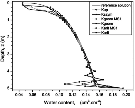
). For the sandy loam n = °2, the critical initial saturation is around 73 %. For hini = - 14 cm and z 25cm, oscillations appear in the evaporation front both the arithmetic and geometric averages. Fig. 7 depicts the profiles of water content with a nodal spacing of 25 cm, an initial saturation of 45% and after 5 days of evaporation. Results differences due to the various conductivity averaging techniques can be observed at the surface of the column because of the variable boundary condition applied and also at the lower part of the soil
mean, the optimized algorithm of Szymkiewicz (2009) and the switching algorithm MS1 which produce monotonic solutions. This trend has been confirmed for the numerous simulations performed with different types of soil, mesh sizes and initial condition. The cumulative evaporation (Qev) and the time to drying (td) are reported in Table 8. These results show that the switching algorithm MS1 provides separate solutions of the upstream mean.
4.2.5. Test problem 5: 2D infiltration in an initially dry sand soil
For multidimensonnal problems, only a few studies have investigated the effect of the equivalent conductivity on the monotonicity and/or accuracy (for instance, Forsyth and Kropinski, 1997; Szymkiewicz and Burzyński, 2011).This problem is studied to evaluate the new algorithm in 2D. We consider a domain of 3 m wide by 3 m deep constituted by sand (soil n = °1 in Table 6) and characterized by the modified van Genuchten model with an air entry pressure of 2 cm. The medium is initially dry (hinit = -1000 cm) and impermeable conditions are applied for all boundaries, except on the top left hand corner
0 x 2m and z=0m
where the infiltration flux is fixed to Q = 2.5 m/day. The infiltration process occurs over 7 days, and the time step size varies heuristically between 1.10-3 s and 360 s.For discretization consisting in quadrangular elements, two grids of 144 elements (25 cm x 25 cm) and 576 elements (12.5 cm x 12.5 cm) respectively are used. A fine grid solution has been computed by considering a 14400-elements-mesh (2.5 cm x 2.5 cm). For rectangular elements, the M-matrix property cannot be verified (Belfort et al., 2009). Hence, this test case allows testing the ability of the different averaging techniques to produce monotonic results. For the computation of equivalent conductivity with the algorithm of Szymkiewicz (2009), a vertical conductivity is determined by using the one-dimensional optimized formulation (see appendix) and a horizontal conductivity is estimated with the
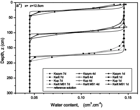
integrated mean. These intermediate conductivities are computed with edges pressure head values. Since the MHFE method involves a single approximation per cell, the equivalent conductivity corresponds to the maximum of the two intermediate conductivies. Fig. 8 illustrates the water content profiles on a vertical segment located at x = 1 m at different times. The arithmetic mean contains oscillations for both grid sizes at time equal to 4 and 7 days. The new algorithm removes these unphysical extremum. Additionally, it appears that the upstream formulation and optimized approach of Szymkiewicz are both free from oscillation. Ɵ-RMSE of the different solutions along the vertical segment are given in Table 9 at different times. The adaptation of the optimized algorithm runs and produces accurate results. Switching algorithm MS1 improves the accuracy of the solutions compared to upstream formulation and leads to specific solutions. With the coarser grid, the solutions obtained with Karit MS1 and Kup are close to each other, mainly at the finale time due to the enlargement of the wetting front and the monotonicity difficulties.
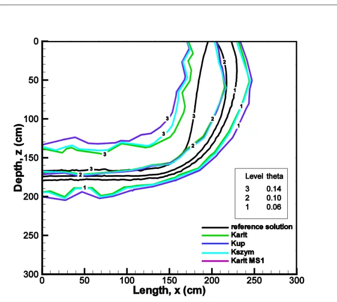
The test case has also been solved with a discretization into triangular elements. A mesh of 225 triangles allows us to study the different formulations compared to a fine mesh solution obtained with 7419 elements. The optimized algorithm is adapted on each cell also by computing to intermediate conductivities. The first step consists in selecting the two edges where the piezometric head is maximum and minimum. Then, Szymkiewicz’s formulation is applied by considering the projection of these two points along the vertical axis. The second intermediate conductivity is the integrated mean constrained by both selected pressure head edge values. The maximum value is kept as the cell equivalent conductivity. If the selected points have the same height, only the second intermediate value is computed. Fig. 9 depicts isolines results obtained after 7 days of infiltration. During the simulation on the coarse grid, the arithmetic formulation provides oscillations and then the upstream mean and the switching algorithm MS1 give rather similar results.
Summary and conclusion
This study focuses on the issue of monotonicity when solving variably saturated flow problems modeled by the non-linear RE. Instead of specifically considering the M-matrix property, the criteria developed by Forsyth and Kropinski (1997) has been used to investigate the monotonicity because it also takes into account the conductivity-averaging method. In the first part of the article, different estimations of Keq. have been presented, including the Darcian mean approximation and optimized algorithm based on the importance of the gravity force (Baker, 2006; Szymkiewicz, 2009). Then, we demonstrate that the integrated formulation remains free from oscillation in the horizontal direction. This result corroborates the conclusion of Pei et al. (2012). The criterion of Forsyth and Kropinski (1997) shows that the upstream method would be the unique unconditional monotonic formulation. We demonstrate that the optimized algorithm developed by Szymkiewicz (2009) satisfy the monotonicity condition for infiltration. To conclude the theoretical part of the study, two switching algorithms are proposed. Both apply the upstream mean if a monotonicity test is not fulfilled during the iterative process for the solution produced by the chosen formulation. In the first approach (MS1), we verify that no unphysical extremum appears in the interior homogeneous part of the domain (without sink / source term). The second algorithm (MS2) adapts the conductivity in function of Forsyth and Kropinski’s condition (Eq. [8] b)).
Various numerical test cases using different material properties, flow conditions and grid sizes are solved. The following concluding remarks can be formulated:
The M-matrix criterion is not sufficient to guaranty monotonicity, and the derivatives of the final matrix system have to be taken into account, which yields a condition dependent on the estimation of the conductivity. This statement holds true for all numerical methods and is not specific to finite volume approach.
Only the upstream formulation satisfies the monotonicity condition for all tested situations. In fact, by comparing our two algorithms, we show that the criterion of Forsyth and Kropinski (1997) is sufficient but not necessary. On the one hand, the use of the upstream mean is reduced with the first approach (MS1) compared to the second one (MS2). On the other hand, punctual applications of the upstream mean allow to ―stabilize‖ the solution.
The deficiencies of traditional averaging techniques have been observed mainly when the nodal spacing increases. Because the upstream formulation is often considered as a diffusive technique, our algorithms represent an alternative solution. Szymkiewicz’s algorithm gives very efficient results; oscillation-free solutions have been obtained during the iterative process and not only at selected printing times.
MS1 algorithm has been implemented in a 2D lumped MHFE method and tested on rectangular and triangular meshes. An andaptation of the optimized algorithm for MHFE equivalent conductivity has also been developed. Preliminar results are satisfactory and avoid unphysical oscillations.
The optimized algorithm developed by Szymkiewicz (2009) is a suitable technique to adapt automatically the conductivity in function of the considered 1D unsaturated flow problem. This technique prevents the development of unphysical oscillations in the solutions of all the test cases performed. Nonetheless, a generalization to different numerical methods in 2D and 3D can be challenging especially for complex / anisotropic geometries (Szymkiewicz, 2013). Beyond the interest of using our switching algorithm MS1 to investigate the issue of monotonicity and relativize the necessity of satisfying the monotonicity criterion of Forsyth and Kropinski (1997), its possible implementation in any numerical code makes it a suitable safety subroutine to avoid oscillations.
Appendix: description and motonicity analysis of Szymkiewicz’s algorithm
1. Presentation of the algorithm and modification
Szymkiewicz (2009) considers that the parameter χ which represents the cosine of the angle between the z axis and the direction of the gravity force is positive. It means that the angle should be comprised between
2
and 2
. Hence, the algorithm has to be modified to
handle all the situations encountered when using a computational code. For instance, a positive upward vertical z axis would lead to numerical difficulties (see description in Figure 2) and the following modifications will be appreciated.
Notations: h hji hjhi, z zji zj zi, U (respectively L) refers to upper (respectively lower) node.
Preliminary: variable ordering to identify upper and lower nodes
if z 0 then hU = hi hL = hj else hU = hj hL = hi end if KU = K(hU)Case 0: Horizontal flow
if 0 then
if h 0 then Keq = KU else
i j h 1 eq i j h K h h .
K h .dh end if return end ifCase 1: Uniform or hydrostatic distribution
if h 0 or h z then Keq = KU
Case 2: Downward flow Situation 1: Infiltration else if h 0 z then
eq 1 2 K max K , K with
U L h 1 U L L U 1 h U L U U 2 h h . K h .dh if h h K K h if h h K K h z
[A.1] Situation 2: Drainage h else if 1 z then
eq 1 2 K min K , K with U 1 2 2 L K K h z h K K h z [A.2]Case 3: Upward flow (Capillary rise)
else
1 2 eq 1 1 1 2 z K K K z z K z K with
L U h z 1 1 L U h K h z h . K h .dh
2 L K K h z
2 2 1 1 2 1 K h 4 1 h z z h K z K 2 1 K end if2. Monotonicity analysis
In this section, we consider that the upper node (subscript U) can be either node j or node i and, to simplify the presentation, we assume that the M-matrix criterion is fulfilled
ij 0
.For infiltration problem:
When using expression K2 of Eq.[1], we obtain Eq.[3] which is always negative. Notice that two expressions can be distinguished (subscripts U and L identify the upper and lower nodes respectively):
r,eq n 1 n 1 n 1 j L ij s n 1 j i ij j r,eq n 1 n 1 n 1 j j U ij s n 1 j i ij ij s ij j j K if h h then K H H A 0 h K K if h h then K H H A K z h h [A.3]Besides, expression K1 in Eq.[A.1] leads to the following expression:
r,eq n 1 n 1 n 1 ji ij s n 1 j i ij ij s j j r,eq j ji K z K H A K K K K 0 h H h [A.4]Which is conditionally negative. Actually, monotonicity of this expression would require:
ji j j r,eq ji z K K K 0 h [A.5]For infiltration, i.e. h 0 z
, Eq. [A.5] implies :
j i h ji r,eq j ji h ji h 1 K K h dh K 1 h z
[A.6]If j corresponds to the lower node and for a large nodal spacing, the integrated formulation can violate Eq. [A.6].
In Szymkiewicz (2009), since Keq corresponds to the maximum of K1 and K2, we demonstrate that the monotonicity condition is therefore fulfilled.
r,eq n 1 n 1 n 1 ji ij s n 1 j i ij ij s j j r,eq j ji K z K H A K K K K h H h Since the hydraulic interblock conductivity is computed from Eq. [A.1], we expect:
U r,eq K K h z and then :
r,eq n 1 n 1 ji U s n 1 j i s r,eq s j j j ji K z K K H K K K K K h h h z H [A.7]Using KU Kjin Eq. [A.7] leads to:
r,eq n 1 n 1 ji s n 1 j i s r,eq s j s j j ji K z 1 K H K K K K 1 1 K K 1 h h h h 1 z z H [A.8] Since h 0 z then Eq. [A.8] gives :
r,eq n 1 n 1 n 1 ij s n 1 j i ij j K K H A 0 h H Consequently, the expression of Eq. [A.1] should respect the monotonicity condition of Eq.[8].
As mentioned for the infiltration case, using expression K2 of Eq. [A.2] allows to satisfy the monotonicity condition.
If
2 LU r,eq L eq LU h K K h K h z , the following equation can be deduced:
eq j L r,eq n 1 n 1 n 1 ji r ij s n 1 j i ij ij s r,eq ji ji j ji h j U r,eq n 1 n 1 n 1 ij ij s n 1 j i ij ij s r,eq ji ji j ij if h h then K h K K H H A K K h z 1 2 h z h if h h then K h K H H A K K 2 h z h z eq r h K h [A.9] For hj = hL, it appears that the sign of Eq. [A.9] depends on the values of theconductivity and its derivative, specifically when ji ji
z
0 h
2 .
Keq corresponds to the minimum of K1 and K2 (Eq. [A.2]), but contrarily to infiltration case, it is not possible to establish the monotonicity of the scheme.
References
An, H., Ichikawa, Y., Tachikawa, Y., Shiiba, M., 2011. A new Iterative Alternating Direction Implicit (IADI) algorithm for multi-dimensional saturated–unsaturated flow. J. Hydrol. 408(1–2), 127-139.
Baker, D.L., 1995. Darcian weighted interblock conductivity means for vertical unsaturated flow. Ground Water 33(3), 385–390.
Baker D.L., 2000. A Darcian integral approximation to interblock hydraulic conductivity means in vertical infiltration. Comput. & Geosci. 26(5), 581-590.
Baker, D.L., 2006. General validity of conductivity means in unsaturated flow models. J. Hydrol. Eng. 11(6), 526-538.
Baker, D.L., Arnold, M.E., Scott, H.D., 1999. Some analytical and approximate Darcian means. Ground Water 37(4), 532-538.
Belfort, B., Carrayrou, J. ,Lehmann, F., 2007. Implementation of Richardson extrapolation in an efficient adaptive time stepping method : applications to reactive transport and unsaturated flow in porous media. Trans. Porous Media 69(1), 123-138.
Belfort, B., Lehmann, F., 2005. Comparison of equivalent conductivities for numerical simulation of one-dimensional unsaturated flow. Vadose Zone J. 4(4), 1191–1200. Belfort, B., Ramasomanana, F., Younes, A., Lehmann, F., 2009. An efficient Lumped Mixed
Hybrid Finite Element formulation for variably saturated groundwater flow. Vadose Zone J. 8(2), 352-362.
Brooks, R. H., Corey, A. T., 1964. Hydraulic properties of porous media. Hydrol. Pap. 3, Colo. State Univ., Fort Collins.
Brunone, B., Ferrante, M., Romano, N., Santini, A., 2003. Numerical simulations of one-dimensional infiltration into layered soils with the Richards’ equation using different
Carsel, R. F., Parrish, R. S., 1988. Developing joint probability distribution of soil water retention characteristics. Water Resour. Res. 24(5), 755– 769.
Celia, M.A., Bouloutras, E.T., Zarba, R.L., 1990. A general mass conservative numerical solution for the unsaturated flow equation. Water Resour. Res. 26(7), 1483–1496.
Chavent, G., Roberts, J.E., 1991. A unified physical presentation of mixed, mixed hybrid finite elements and standard finite difference approximations for the determination of velocities in water flow problems. Adv. Water Resour. 14(6), 329–348.
Cooley, R.L., 1983. Some new procedures for numerical solution of variably saturated flow problems. Water Resources Res. 19(5), 1271-1285.
Crevoisier, D., Chanzy, A., Voltz, M., 2009. Evaluation of the Ross fast solution of Richards’ equation in unfavourable conditions for standard finite element methods. Adv. Water Resour. 32(6), 936-947.
Farthing, M.W., Kees, C.E., Miller, C.T., 2003. Mixed finite element methods and higher order temporal approximations for variably saturated groundwater flow. Adv. Water Resour. 26(4), 373-394.
Forsyth, P.A., Kropinski, M.C., 1997. Monotonicity considerations for saturated-unsaturated subsurface flow. Siam J. Sci. Comput. 18(5), 1328-1354.
Forsyth, P.A., Wu, Y.S., Pruess, K., 1995. Robust numerical methods for saturated-unsaturated flow with dry initial conditions in heterogeneous media. Adv. Water Resour. 18(1), 25-38.
Fuentes, C., Haverkamp, R., Parlange, J.-Y., 1992. Parameter constraints on closed-form soil-water relationships. J. Hydrol. 134(1-4), 117– 142.
Gardner, W.R., 1958. Some steady-state solutions of the unsaturated moisture flow equation with application to evaporation from water table. Soil Sci. 85(4), 228–232.
Gastó, J.M., Grifoll, J., Cohen, Y., 2002. Estimation of intermodal permeabilities for numerical simulation of unsaturated flows. Water Resour. Res. 38(12), 1326.
Haverkamp, R., Vauclin, M., 1979. A note on estimating finite difference interblock hydraulic conductivity values for transient unsaturated flow problems. Water Resour. Res. 15(1), 181-187.
Haverkamp, R., Vauclin, M., Touma, J., Wierenga, P.J., Vachaud, G., 1977. A comparison of numerical simulation models for one-dimensional infiltration. Soil Sci. Soc. Am. J. 41(2), 285-294.
Hoteit, H., Mose, R., Philippe, B. Ackerer, P., Erhel, J., 2002. The maximum principle violations of the mixed-hybrid finite-element method applied to diffusion equations. Int. J. Numer. Meth. Eng. 55(12), 1373–1390.
Huyakorn, P., Thompson, S., Thompson, B., 1984. Techniques for making finite element methods competitive in modelling flow in variably saturated porous media. Water Resour. Res. 20(8), 1099-1115.
Ippisch, O., Vogel, H.-J., Bastian, P., 2006. Validity limits for the van Genuchten–Mualem model and implications for parameter estimation and numerical simulation. Adv. Water Resour. 29(12), 1780–1789.
Ju, S.-H., Kung, K.-J.S., 1997. Mass types, element orders and solution schemes for the Richards equation. Comput. Geosci. 23(2), 175–187.
Karthikeyan, M., Tan, T.S., Phoon, K.K., 2001. Numerical oscillation in seepage analysis of unsaturated soils. Can. Geotech. J. 38(3), 639-651.
Kuráž, M., Mayer, P., Lepš, M., Trpkošová, D., 2010. An adaptive time discretization of the classical and the dual porosity model of Richards’ equation. J. Comput. Appl. Math. 233(12), 3167-3177.
Lassabatere, L., Angulo-Jaramillo, R., Soria Ugalde, J. M., Cuenca, R., Braud, I., Haverkamp, R., 2006. Beerkan estimation of soil transfer parameters through infiltration experiments—BEST. Soil Sci. Soc. Am. J. 70(2), 521– 532.
Lehmann, F., Ackerer, Ph., 1998. Comparison of iterative methods for improved solutions of the fluid flow equation in partially saturated porous media. Trans. Porous Media 31(3), 275-292.
Lott, P.A., Walker, H.F., Woodward, C.S., Yang, U.M., 2012. An accelerated Picard method for nonlinear systems related to variably saturated flow. Adv. Water Resour. 38, 92-101. Loudyi, D., Falconer, R.A., Lin, B., 2007. Mathematical development and verification of a non-orthogonal finite volume model for groundwater flow applications. Adv. Water Resour. 30(1), 29-42.
Manzini, G., Ferraris, S., 2004. Mass-conservative finite volume methods on 2-D unstructured grids for the Richards’ equation. Adv. Water Resour. 27(12), 1199–1215.
Miller, C. T., Williams, G. A., Kelley, C. T., Tocci, M. D., 1998. Robust solution of Richards’ equation for nonuniform porous media. Water Resour. Res. 34(10), 2599–2610.
Milly, P.C.D., 1985. A mass-conservative procedure for time-stepping models of unsaturated flow. Adv. Water Resour. 8(1), 32–36.
Milly, P.D.C., 1988. Advances in Modeling of Water in the Unsaturated Zone. Trans. Porous Media 3, 491-514.
Neuman, S.P., 1972. Finite element computer programs for flow in saturated-unsaturated porous media. second annual report, A10-SWC-77, Hydraul. Eng. Lab., Technion, Haïfa, Israël.
Oldenburg, C.M., Pruess, K., 1993. On numerical modeling of capillary barriers. Water Resour. Res. 29(4), 1045–1056.
Pan, L., Warrick, A.W., Wierenga, P.J., 1996. Finite element methods for modeling water flow in variably saturated porous media: Numerical oscillation and mass-distributed schemes. Water Resour. Res. 32(6), 1883–1889.
Pei, Y.S., Yang, Z.F., Zhang, K.J., Tian, B.H., 2012. Deficiency of Approximate Interblock Conductivities for Simulation of Horizontal Unsaturated Flow. Transp. Porous Med. 91, 627–647.
Raats, P.A.C., 2001. Developments in soil–water physics since the mid 1960s. Geoderma 100(3–4), 355-387.
Rathfelder, K., Abriola, L. M., 1994. Mass conservative numerical solutions of the head-based Richards equation. Water Resour. Res. 30(9), 2579-2586.
Rawls, W. J., Brakensiek, D. L., Saxton, K. E., 1982. Estimation of soil water properties. Trans. ASAE 25(5), 1316-1320.
Romano, N., Brunone, B., Santini, A., 1998. Numerical analysis of onedimensional unsaturated flow in layered soils. Adv. Water Resour. 21(4), 315-324.
Russo, D., 1988. Determining soil hydraulic properties by parameter estimation: On the selection of a model for hydraulic properties. Water Resour. Res. 24(3), 453-459.
Sandhu, R.S., Liu, H., Singh, K.J., 1977. Numerical performance of some finite element schemes for analysis of seepage in porous elastic media. Int. J. Numer. Anal. Meth. Geomech. 1(2), 177–194.
Schaap, M. G., Leij, F. J., 2000. Improved prediction of unsaturated hydraulic conductivity with the Mualem – van Genuchten model. Soil Sci. Soc. Am. J. 64(3), 843–851.
Schnabel, R.R., Richie, E.B., 1984. Calculation of internodal conductancess for unsaturated flow simulations: A comparison. Soil Sci. Soc. Am. J. 48(5), 1006–1010.
Schweizer, B., 2012. The Richards equation with hysteresis and degenerate capillary pressure. J. Differ. Equations. 252(10), 5594-5612.
![Figure 2. Steady state tests: percentage of minimum value of the coefficient of Eq. [12]](https://thumb-eu.123doks.com/thumbv2/123doknet/14796520.604076/41.892.131.753.213.1129/figure-steady-state-tests-percentage-minimum-value-coefficient.webp)