HAL Id: hal-00443057
https://hal.archives-ouvertes.fr/hal-00443057
Submitted on 21 Aug 2015
HAL is a multi-disciplinary open access
archive for the deposit and dissemination of
sci-entific research documents, whether they are
pub-lished or not. The documents may come from
teaching and research institutions in France or
abroad, or from public or private research centers.
L’archive ouverte pluridisciplinaire HAL, est
destinée au dépôt et à la diffusion de documents
scientifiques de niveau recherche, publiés ou non,
émanant des établissements d’enseignement et de
recherche français ou étrangers, des laboratoires
publics ou privés.
related to early spring transport of mid-latitude sources
into the Arctic
Raphaël Adam de Villiers, Gérard Ancellet, Jacques Pelon, Boris Quennehen,
Alfons Schwarzenboeck, Jean-François Gayet, Kathy S. Law
To cite this version:
Raphaël Adam de Villiers, Gérard Ancellet, Jacques Pelon, Boris Quennehen, Alfons Schwarzenboeck,
et al.. Airborne measurements of aerosol optical properties related to early spring transport of
mid-latitude sources into the Arctic. Atmospheric Chemistry and Physics, European Geosciences Union,
2010, 10 (11), pp.5011-5030. �10.5194/acp-10-5011-2010�. �hal-00443057�
doi:10.5194/acp-10-5011-2010
© Author(s) 2010. CC Attribution 3.0 License.
Chemistry
and Physics
Airborne measurements of aerosol optical properties related to early
spring transport of mid-latitude sources into the Arctic
R. A. de Villiers1, G. Ancellet1, J. Pelon1, B. Quennehen2, A. Schwarzenboeck2, J. F. Gayet2, and K. S. Law1
1UPMC Univ. Paris 06; Universit´e Versailles St-Quentin; CNRS/INSU, LATMOS-IPSL, France 2Laboratoire de M´et´eorologie Physique, Universit´e B. Pascal, CNRS, France
Received: 1 December 2009 – Published in Atmos. Chem. Phys. Discuss.: 23 December 2009 Revised: 13 April 2010 – Accepted: 12 May 2010 – Published: 1 June 2010
Abstract. Airborne lidar and in-situ measurements of the aerosol properties were conducted between Svalbard Island and Scandinavia in April 2008. Evidence of aerosol trans-port from Europe and Asia is given. The analysis of the aerosol optical properties based on a multiwavelength li-dar (355, 532, 1064 nm) including volume depolarization at 355 nm aims at distinguishing the role of the different aerosol sources (Siberian wild fires, Eastern Asia and European an-thropogenic emissions). Combining, first aircraft measure-ments, second FLEXPART simulations with a calculation of the PBL air fraction originating from the three different mid-latitude source regions, and third level-2 CALIPSO data products (i.e. backscatter coefficient 532 nm,volume depolar-ization and color ratio between 1064 and 532 nm in aerosol layers) along the transport pathways, appears a valuable ap-proach to identify the role of the different aerosol sources even after a transport time larger than 4 days. Optical depth of the aerosol layers are always rather small (<4%) while transported over the Arctic and ratio of the total attenuated backscatter (i.e. including molecular contribution) provide more stable result than conventional aerosol backscatter ra-tio. Above Asia, CALIPSO data indicate more depolariza-tion (up to 15%) and largest color ratio (>0.5) for the north-eastern Asia emissions (i.e. an expected mixture of Asian pollution and dust), while low depolarization together with smaller and quasi constant color ratio (≈0.3) are observed for the Siberian biomass burning emissions. A similar dif-ference is visible between two layers observed by the air-craft above Scandinavia. The analysis of the time evolution of the aerosol optical properties revealed by CALIPSO be-tween Asia and Scandinavia shows a gradual decrease of
Correspondence to: G. Ancellet
(gerard.ancellet@upmc.fr)
the aerosol backscatter, depolarization ratio and color ratio which suggests the removal of the largest particles in the ac-cumulation mode. A similar study conducted for a European plume has shown aerosol optical properties intermediate be-tween the two Asian sources with color ratio never exceeding 0.4 and moderate depolarization ratio being always less than 8%, i.e. less aerosol from the accumulation mode.
1 Introduction
Radiative effects of aerosols can be quite different in the Arctic compared to elsewhere (Quinn et al., 2008). Weakly absorbing aerosol layers can be effective for heating the earth-atmosphere system considering the high surface albedo (Pueschel and Kinne, 1995). Frequent haze and cloud layers in the winter-spring period contributes also to surface heating by their infrared emission (Garrett and Zhao, 2006). Cloud formation processes are also very sensitive to the aerosol properties as Arctic clouds often contain low droplet concen-trations. Shindell et al. (2008) have examined multi-model results to assess the aerosol and CO transport to the Arctic. They underline in their work the major role played by Euro-pean and East Asian emissions especially in winter. There is also a very significant altitude dependence of the Arctic sensitivity to emission change. The relative influence of the different mid-latitude aerosol sources was already discussed by Rahn (1981) who concluded using meteorological con-siderations and observations about the relative importance of the Eurasian transport pathway. The review of Law and Stohl (2007) has also stressed the seasonal change of the air pollution transport into the Arctic with a faster winter circu-lation implying a stronger influence of the southerly sources.
Because of the strong low level winter transport barrier, these emissions are found in the middle and upper troposphere.
Two measurement campaigns in the Arctic took place dur-ing the sprdur-ing season: TOPSE (Atlas et al., 2003) over the North American sector and ASTAR over the European sec-tor (Engvall et al., 2008). Over the European Arctic secsec-tor, the ASTAR results have shown low level of aerosol particles even in layers with elevated CO, suggesting aerosol removal in clouds. Occurrence of layers of non volatile and aged aerosol however increases with altitude in this region. The conditions during the ASTAR-2007 experiment were how-ever exceptionally clean and other studies show events with large amount of polluted air masses in the lower troposphere, e.g. in spring 2006 (Stohl et al., 2007a).
Over the North American Arctic sector, little evidence was found for new particle formation (Weber et al., 2003) dur-ing TOPSE. The question of the relative influence on con-densation nuclei of this low production rate and import from mid-latitudes could not be clearly assessed. Sulphate aerosol particles and more generally haze layers became more preva-lent at higher altitudes across the winter to spring transition period during the TOPSE experiment (Scheuer et al., 2003). The aerosol lidar data during TOPSE (Browell et al., 2003) were mainly used to establish a link between the ozone and aerosol trends during the winter-spring transition, but some evidence was given of the role of the Eurasian sources on the observed aerosol optical properties.
Considering the crucial role of European and Asian emis-sion suggested by the model studies and a significant altitude dependence of the occurrence of aerosol layers, new aircraft observations were conducted in 2008 at the same time over the European Arctic and North American sector to clarify questions raised during the previous campaigns (Jacob et al., 2009).
The purpose of this paper is to discuss how a backscat-ter lidar, in-situ aerosol and CO observations obtained over the European Arctic sector can be combined with a trans-port model and spaceborne measurements by the CALIOP lidar in order to get a better understanding of the aerosol source attribution in this region. This kind of methodology is also very useful for studying the aerosol evolution during the long range transport. Therefore, we focus on a given flight (11 April 2008), which is a very good example of the me-teorological conditions encountered during the POLARCAT-France spring campaign. A short description of the POLAR-CAT (Polar Study using Aircraft, Remote Sensing, Surface Measurements and Models, of Climate, Chemistry, Aerosols, and Transport) campaign is given in Sect. 2. A more de-tailed description of the campaign achievements is planned in a forthcoming publication by Law et al. (2010). Our pa-per focuses on lidar data as they are especially useful to de-scribe the vertical layering of the atmosphere and to derive the optical properties of the aerosol layers. We will analyze the complementarity of optical aerosol characterization and transport modeling studies for making source attribution of
Arctic tropospheric aerosol. A Lagrangian approach using aircraft observations and a model for the study of the long range transport is indeed a well established method for the analysis of observations at mid-latitudes (Fehsenfeld et al., 2006; Stohl et al., 2007b). But the main advantage of the POLARCAT campaign is to rely also on range resolved satel-lite observations by the CALIOP lidar providing aerosol lay-ers optical properties at two different wavelength (532 nm, 1064 nm). Our airborne lidar data must be analyzed using aerosol layer products similar to the CALIOP observations (Liu et al., 2009). This work also contributes to check how meaningful the CALIOP operational aerosol layer products are.
2 Aircraft data and meteorological context 2.1 The POLARCAT spring campaign
In 2008, two aircraft field campaigns have been successfully performed: the first one in Kiruna (68◦N, 20◦E, North Swe-den) in March–April and the second one in Kangerlussuaq (Greenland) in July. The ATR-42 was equipped with remote sensing instruments (lidar, radar), in-situ measurements of gas (O3, CO) and aerosols (Aerosol Mass Spectrometers,
op-tical counters, size distribution). Cloud properties were anal-ysed using a Counterflow Virtual Impactor (CVI). The flight strategy was often designed to collect data nearby satellite observations (Aqua-Train, Metop/IASI).
During the spring campaign the objectives were (i) char-acterization of the pollution transport, (ii) analysis of the aerosol/cloud interaction, (iii) satellite validation, and (iv) studies of the artic haze. The latter could not be addressed as sampling of the air masses North of the Arctic front was not possible with the limited range of the ATR-42. A set of 12 scientific flights was performed from 30 March to 11 April 2008 following more or less a South-North axis near 20◦E. A first contribution of POLARCAT was to combine aerosols and cloud droplets characterization to understand the aerosol/cloud interaction. The second major achieve-ment was to identify numerous well defined aerosol layers in the free troposphere related to long range pollution trans-port. The third important result is the large number of flights conducted near the CALIPSO tracks. In the present paper, the second and third topics, will be addressed. Generally speaking this period was characterized by frequent north-ward transport of the European pollution and even the sam-pling of Asian pollution transported across the pole from 9 April to 11 April. To discuss the methodology developed in the paper, (i.e. a joint analysis of the aerosol airborne li-dar data with CALIOP observations and FLEXPART mod-elling), we will focus on the results of 11 April 2008, because they include the two kinds of aerosol layers encountered dur-ing the POLARCAT sprdur-ing campaign.
2.2 Flight description and meteorological context On April 11, 2008, the ATR-42 flew from Kiruna to the latitude circle at 73◦N. The purpose of this flight was to sample two kinds of air masses: one transported across the North Pole to Northern Scandinavia and the other one ex-ported from Europe by mid-latitude weather systems. The Lagrangian FLEXPART model, used in a forecast mode (Stohl et al., 2004), indeed showed a well defined CO plume at 72◦N and suggested long range transport of mid-latitude emissions. The meteorological situation can be described using the wind field at 700 hPa and the vertical cross sec-tion of the specific humidity at 20◦E along the flight pattern (Fig. 1). It shows that the aircraft measurements were col-lected between two frontal zones at 68◦N and 74◦N. The wind field indicates a weak southerly flow in the southern part of the domain but then a well defined northerly flow at latitudes higher than 70◦N. Assuming advection along the isentropic surfaces in the free troposphere, the northerly flow also corresponds to a downward motion in the 3–6 km alti-tude range. We can also notice that, further east at 30◦E, the
flow at northern latitudes remains southerly and intensifies. The corresponding flow curvature is related to the positive vorticity anomaly located at 25◦E south of Spitzbergen. A flight in the latitude band 68◦−72◦N is then interesting as its southern section characterizes an upward and northward flow corresponding to a fast and direct export from Europe, while its northern section samples the downward branch of the Arctic outflow with aged mid-latitude emissions accord-ing to the FLEXPART forecast. The red solid line in Fig. 1 corresponds to the aircraft vertical profile. During the first part of the flight between 10:00 UT and 11:30 UT, the air-craft flew above 3 km before a descent to explore the Arctic planetary boundary layer (PBL) at 72.5◦N. During the sec-ond part of the flight, i.e. the return to Kiruna, the aircraft stayed within the PBL for aerosol-cloud interaction studies and made a second exploration of the free troposphere for latitude below 70.5◦N. So, in addition to lidar data below the aircraft, four complete vertical profiles of the aerosol concen-trations are derived from the in-situ measurements between 0 and 5.5 km.
2.3 Lidar measurements
2.3.1 Description of the lidar system
The new version of the LEANDRE airborne backscatter li-dar currently used for atmospheric dynamics studies (Fla-mant et al., 1996) and aerosol characterization (Pelon et al., 2002) is now providing measurements of total attenuated backscatter vertical profiles at three wavelengths (355, 532 and 1064 nm). The additional channel at 355 nm is now used to measure cross-polarization attenuated backscatter profiles. The main lidar characteristics are summarized in Table 1.
Fig. 1. Vertical cross section of ECMWF specific humidity showed
by the color coded contour in ppmM, potential temperature in K showed by black dashed lines (top panel) and ECMWF wind field at 700 hPa (bottom panel) on 11/04/2008 at 12:00 UT. The colored lines show the windspeed in m s−1. The flight vertical and horizon-tal pattern are showed in red line.
The 355-nm pseudo depolarization ratio, δ355, i.e. the ratio
of the the total perpendicular- to the total parallel-polarized backscatter coefficient (see Appendix A) is calculated in or-der to have a parameter comparable with the CALIOP vol-ume depolarization ratio which is also based on the ratio of the total backscatter coefficient (Winker et al., 2009). The latter is however given at 532-nm and one must account for the spectral variation of this ratio from 355 nm to 532 nm
Table 1. Airborne Lidar data characteristics.
Operation Wavelengths (nm) 355 (Parallel and PP) 532 1064 Emitted energy (rep rate 20 Hz) 50 mJ 10 mJ 80 mJ Laser Divergence (FWHM) 0.16 mrd 4 mrd 6.5 mrd
Spot size @5 km 0.8 m 20 m 33 m
Filter Width (FWHM) 5 nm 0.2 nm 1 nm Max. Filter Transmission (%) 25 25 30
Telescope diameter 30 cm
Time Sampling and vertical resolution 20 MHz or 7.5 m Vertical resolution used 30 m (4 points) Horizontal separation (shot-to-shot) 4–5 m (at ATR 42 cruise speed) Horizontal resolution used ∼450 m (100 shots)
when comparing aircraft and satellite observations . For ex-ample, we can assume that the aerosol depolarization val-ues weakly vary between 355 and 532 nm as explained in Appendix A (Freudenthaler et al., 2009; Sugimoto and Lee, 2006).
The pseudo depolarization ratio is calibrated on molecular scattering. From the values reported in Table 1, one can see that the interference filter width at 355 nm is much larger than the Cabannes line of the molecular backscattered signal and includes all Raman rotational lines due to nitrogen and oxy-gen which are the main scattering gases in the atmosphere (see Fig. 2 of Radlach et al. , 2008). Consequently, we will use the total Rayleigh+Raman depolarization value in clean air. We have adopted the value of 1.5 10−2(Hostetler et al., 2006). Due to noise in normalization and possible biases, the error on the derived values is estimated to be 20%.
For the same reason, i.e. a comparison with the CALIOP aerosol layer products, the pseudo color ratio which is the ratio of the 1064-nm to the 532-nm total backscatter coeffi-cient, is calculated as it is a mean to identify aerosol type. Al-though this ratio is comparable to the CALIOP aerosol layer products (Winker et al., 2009), it will requires further cor-rection for attenuation above the altitude of the aircraft as discussed later. The pseudo color ratio can be related to the aerosol color ratio more currently used for such a purpose (Cattrall et al., 2005). Details are given in Appendix A.
For the relative comparison between the aerosol layers properties seen by the airborne lidar and the comparison with the CALIOP observations, we will use the pseudo ratios.The main advantage of the pseudo ratios is to provide quasi-direct comparisons. As it accounts for molecular scattering, it leads to more stable values for weak aerosol layers and therefore relative comparisons are more robust. It however introduces a dependence with the scattering ratio (see Appendix A), which may in some cases lead to difficulties in interpretation. We thus have also given values of the standard parameters in the next sections for the strongest aerosol layers, which helps our analysis to be more comparable to previous studies.
2.3.2 Aerosol lidar data on 11 April 2008
A vertical cross section of the total attenuated backscatter in the infra-red (IR) channel is shown in Fig. 2. The areas with very large backscatter in the altitude range 1–2 km cor-respond to cloud layers developing at the top of the Plane-tary Boundary Layer (PBL). The cloud top reaches 3 km as the aircraft approaches the Arctic front. In the cloud free area, the layer from 0 to 1 km with larger aerosol backscat-ter values corresponds to the PBL. Well defined layers with enhanced aerosol backscatter are also detected in the free troposphere. The layer with a depth less than 1 km and with a meridian extent between 70◦N and 72.5◦N has the strongest relative signal compared to the background aerosol in the IR. This layer has also a slight vertical tilt, probably corresponding to the tilt of the isentropic surface. Another aerosol plume is also seen at latitudes less than 69.2◦N, but
with a much larger altitude range between 3.5 and 5.5 km and weaker backscatter at 1064 nm.
To further characterize these two layers, four 20-s averages of lidar profiles were analyzed: the first one corresponds to the thick layer at 68.9◦N (named layer I hereafter), the sec-ond and third ones are through the longest and thin layer at 69.6◦N and 71.7◦N (layer II-A and II-B) and the last one at 70.6◦N samples the cloud free marine PBL over the Arctic ocean. The attenuated backscatter ratio, R(z), is de-fined in this paper as the Rayleigh normalized total volume backscatter, only attenuated by the aerosol extinction (see Appendix A). It was derived from vertical profiles averaged over the 4 selected regions, and applying a calibration fac-tor to reference the scattering ratio to 1 in clean air. This factor was calculated using areas with mainly Rayleigh con-tribution to the IR lidar signal in the altitude range close to the aircraft (e.g. at 69.6◦N above 5 km or at 70.3◦N near 3 km). This was done independently for each wavelength and the consistency of the calibration factor is checked us-ing different aerosol free areas whenever possible. This is the major source of error in the calculation of R(z), and the uncertainty was assumed to be less than 10% at 532 nm and 355 nm, less than 20% at 1064 nm. The latter was derived
Fig. 2. Vertical cross section of the attenuated 1064 nm backscatter measured by downward looking lidar between 68◦N and 72.5◦N. The white vertical lines represent the four profiles, I, II-A, PBL, and II-B.
Fig. 3. Lidar vertical profiles of the 20-s averages of the attenuated backscatter ratio at 355, 355 depolarized, 532 and 1064 nm for the 4 lidar
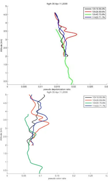
Fig. 4. Vertical profiles of the 355 nm pseudo depolarization ratio
δ355and the pseudo color ratio between 1064 and 532 nm for the 4
lidar profiles listed in Table 2 and showed by the white bar in Fig. 2
from a sensitivity study using different possible calibration factors and different flights.
The R(z) vertical profiles for each wavelength and the 4 selected latitudes are given in Fig. 3. For the strongest aerosol layer at 69.6◦N (layer II-A), the R increase is present in the three wavelength channels. The maximum
R value at 532 nm is of the order of 2 and it corresponds to a 532-nm aerosol backscatter coefficient of the order of 10−3km−1sr−1and therefore a small optical depth for layer II-A (≈ 3-4 10−2) assuming a 532-nm lidar ratio of the order of 70 sr (Cattrall et al., 2005), i.e. considering for example biomass burning aerosol. For the other layers (I and II-B),
R is of the order of 2 at 1064 nm and between 1.3–1.4 at 532 nm. Layers with IR values of R less than 1.5 will not be considered in the following discussion.
Fig. 5. Vertical profiles of the aerosol color ratio between 1064 and
532 nm and its standard deviation for the largest layers observed by the airborne lidar at 68.6◦N 68.9◦N 70.6◦N and 71.7◦N.
The pseudo depolarization ratios δ355 are shown for the
four profiles (Fig. 4a) and it becomes significantly larger than the molecular depolarization only for the layer II-A at 69.6◦N near 3.2 km where it is of the order of 0.021. No-tice that it is also larger than the Rayleigh depolarization in the Arctic PBL (0.019). For the layer II-A, the aerosol de-polarization ratio, corresponding to a δ355of 0.021, is of the
order of 3.3%, i.e. a value much smaller than the 532-nm aerosol depolarization ratio reported by Gobbi et al. (2003) for a mountain site in Italy. This would be consistent with a significant fraction of spherical aerosol even though we are able to detect some depolarization in layer II-A.
The pseudo color ratio plot for the four profiles shows also largest values (0.13±0.01) in layer II-A at 69.6◦N (Fig. 4b). The smaller values (0.08±0.02) in the southern layer are con-sistent with the hypothesis of smaller aerosol size in layer I. The pseudo color ratio in layer II-B at 71.7◦N near 3.5 km (0.11±0.02) is intermediate between the two previous cases. The main characteristics of the aerosol layers identified in Fig. 3 are listed in Table 2 with the expected uncertainty on the pseudo color and depolarization ratio. The aerosol color ratio, which is proportional to (R1.06−1)/(R0.53−1), is also
listed in Table 2 as it is generally directly linked to the aerosol backscatter wavelength dependency and reported in previous studies on tropospheric aerosols (see Appendix A for differ-ences between the two ratios).
For all the layers,our values of color ratios are much smaller than the reported values of Cattrall et al. (2005). In their work, the color ratios are calculated using data from the AERONET photometer worldwide network at 550 and 1020 nm, and for larger aerosol optical depths (>0.1). Their values are ranging between 0.5 (polluted layers) to 1 (dust layers), whereas the Angstrom coefficient determined from
Table 2. Aerosol layer characteristics from the airborne lidar observations.
Lidar Layer Altitude β532 Aerosol Pseudo Aerosol Pseudo
layer latitude range, km km−1sr−1 color ratio color ratio δ355 δ355
I 68.9◦N 3.5–4.5 1.2±0.1 10−3 0.21±0.14 8.5±1.8 10−2 2.1±1.8% 1.6±0.3% II-A 69.6◦N 2.8–3.8 2.2±0.2 10−3 0.19±0.03 12.5±1.3 10−2 3.3±0.9% 2.1±0.3% PBL 70.6◦N <0.8 1.8±0.2 10−3 0.24±0.12 10.4±1.7 10−2 5.4±5.3% 1.9±0.3% II-B 71.7◦N 3.5–4.5 1.3±0.1 10−3 0.20±0.06 11±1.6 10−2 2.1±1% 1.6±0.2%
extinction coefficients decreases from 2 to 0. This is com-parable to calculations made from the Optical Properties of Aerosols and Clouds (OPAC) package (Hess et al., 1998; Liu et al., 2004). For our observations, corresponding to smaller aerosol optical depths (<0.04) and small backscatter coeffi-cients (1–2 10−3km−1sr−1), the color ratio is about 0.2, for all the layers, as reported in Table 2 and in Fig. 5. This cor-responds to a wavelength dependence in the backscatter co-efficient larger than 2, indicative of small particle sizes. The pseudo color ratio shows slightly smaller values for layer I, with respect to the other ones, but looking at the variability, it does not appear to be fully significant, and no major dif-ference is seen on color ratio (Fig. 5). The overall results of Table 2 however show that the apparently homogeneous layer II may be formed of several aerosol sources since layer II-A and II-B have different optical characteristics. To sumarize, the airborne lidar data show that:
– aerosol layers are identified in the mid-troposphere hav-ing very low optical depths (<0.04).
– two layers (I and II) are detected with markedly differ-ent vertical structure and backscatter values implying different aerosol sources and probably different trans-port processes
– layer I has low depolarization and lowest pseudo color ratio related to a very small fraction of coarse size par-ticles
– layer II is not homogeneous with, according to the pseudo color ratio values, larger particles than layer I and even some depolarization in layer II-A.
– pseudo color ratio and aerosol color ratio are smaller than values derived from the AERONET network, mainly because of larger Angstrom coefficient in our study.
To get more insight in the airborne lidar data indications, we have taken advantage of the flight pattern to analyze the in-situ measurements when the aircraft has crossed the layers observed by the lidar.
2.4 In-situ measurements
Ozone and carbon monoxide (CO) were measured on the ATR-42 (Nedelec et al., 2003). The CO is especially useful as it can indicate if an air mass has been influenced by com-bustion processes less than 10–20 days before. Regarding the aerosol concentrations, an optical counter (CPC-3010) mea-sured the number of submicronic particles with sizes larger than 10 nm and a Passive Cavity Aerosol Spectrometer Probe (PCASP SPP-200) provided the number of particles in 30 size bins between 0.1–3 µm. Uncertainties up to 10% have to be taken in account because of difficulties to estimate the correct probe volumic sample flow. In this paper the PCASP data are summed over all the size bins to get a concentration number comparable to the optical counter. Differences be-tween the two numbers are mostly related to a large fraction of small particles (<100 nm) detected by the optical counter but not seen by the PCASP.
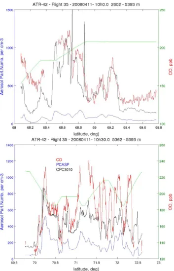
The CO and the aerosol concentrations from the PCASP and the CPC are shown in Fig. 6 for latitudes lesser and greater than 70◦N, respectively the second plot correspond-ing to the numerous crosscorrespond-ing of the layer II identified by the lidar. The CO variability is generally well correlated with the aerosol concentrations is of the order of 100 ppb. It is not very different for the southerly flow and the Artic out-flow. This variability can be explained by the highly stratified aerosol and chemical composition of the free troposphere as shown by the lidar. The smallest CO values around 130 ppb correspond to the cleanest and oldest air masses, sampled on this flight.
When comparing the PCASP and the optical counter data, one can notice higher concentrations of small particles in the southern section of the flight. This is related to either the removal of larger particles during the transport from mid-latitudes or to the generation of new smaller particles. The two hypotheses imply differences for layer I and II in the air mass age since exposure to emissions or in the nature of the emissions (e.g. more SO2 concentrations, Weber et al.
(2003) or more organic emissions from continental regions over Northern Europe, Sellegri et al., 2005). A more direct way to demonstrate the larger fraction of very small particles is to plot the size spectrum measured along the flight by a Scanning Mobility Particle Sizer (SMPS) for particle smaller than 300 nm and the PCASP for larger particles (Fig. 7).
Fig. 6. CO (red) and aerosol concentrations for the PCASP (blue)
and CPC (black) along the fligth track for latitudes <70◦N (top panel) and latitudes >70◦N(bottom panel). Aircraft altitude di-vided by a factor 5 (green) is plotted in m using the left vertical axis.
It shows indeed smaller particle sizes (30–200 nm) for the southern section of the flight, while the Artic outflow corre-sponds to larger particles (100–300 nm). This is consistent with the interpretation of the differences between the PCASP and the optical counter. It is also noticeable that the fraction of particles with a diameter exceeding 300 nm are increasing in the layer II-A at 69.6◦N, i.e. where the pseudo color and
depolarization ratio are maximum in the lidar data.
The analysis of the in-situ data therefore sheds light on interpretation of the lidar data and we can say that:
– the lidar aerosol layers are mostly related to either biomass burning or urban/industrial sources consider-ing the good correlation between aerosol and CO con-centrations. This was already reported in Kampe and Sokolik (2007) and Capes et al. (2008).
Fig. 7. Size spectrum (nm) measured as a function of time along the
flight track by the SMPS (0.01 and 0.4 µm) and PCASP (0.4–3 µm). The vertical flight pattern is showed for comparaison with latitude cross-section (black line) in Figs. 13 and 2.
– the pseudo color ratio analysis is consistent with the observed aerosol size distribution showing the largest aerosol size for the layer II-A, even though the aerosol optical depth is small and the variability of this ratio is weak.
To understand the respective influence of the aging and the nature of the sources, air mass origins were investigated us-ing transport modelus-ing.
3 Modeling of the transport to the Arctic 3.1 Description of the FLEXPART simulations
The origin of the observed air masses was studied using the Lagrangian Particle Dispersion Model (LPDM) FLEX-PART version 6 (Stohl et al., 1998, 2002) driven by 6-hourly ECMWF analyses (T213L91) interleaved with oper-ational forecasts every 3 h. In addition to classical advec-tion, the LPDM includes turbulent diffusion, parameteriza-tions of sub-grid scale convection and of topographic pro-cesses, as well as online computation of potential vorticity (PV) for each air parcel. The fraction of particles with PV
>2 PVU (1 PVu=10−6kg−1m2) is calculated as a function of time to estimate the probability of transport from or into the stratosphere. Previous studies have shown that a frac-tion larger than 20% corresponds to a significant influence of the stratosphere-troposphere exchange (STE) processes. We modified the FLEXPART model to introduce the calcu-lation of the fraction of particles originating below an altitude of 3 km, for three areas corresponding to different emissions of particulate matter and CO: Europe (latitude <55◦N, lon-gitude ∈ [−10◦W 30◦E]), Asia (latitude <55◦N, longitude
Fig. 8. Meridional vertical cross section of air mass origins
cal-culated by Flexpart for 500 m×0.5◦×0.5◦ boxes. The color scale indicates the fraction of particles in % being in the European (first figure) and Asian (second figure) lower troposphere (z63 km), 5
days before the observations. Aircraft altitude is shown in white.
∈ [30◦E 180◦E], North America (latitude <55◦N, longitude
∈ [−180◦W −30◦W]).
Next we divided the lidar vertical cross-section of Fig. 2 in 130 boxes with the following size: depth of 500 m and hori-zontal size of 0.5◦×0.5◦. For each box, 2000 particles were
released during 60 min and the dispersion computed for 7 days backward in time. As we focus on layers, our aim is to document their history as long as they remain coherent, i.e. before they undergo strong mixing which, as reported by Methven et al. (2006), becomes significant after 4 days for trajectories arriving above western Europe. The vertical cross-section of the air mass origin can be reconstructed us-ing a plot of the fraction of particles beus-ing in the lower tro-posphere of a given region 5 days before the lidar
observa-Fig. 9. 5-days FLEXPART backward time position of five clus-ters of the 2000 particles released between 4 and 4.5 km at 68.6◦N (top panel) and between 3.5 and 4 km at 72.1◦N (bottom panel) on 11/04/2008 at 12:00 UT. The clusters are plotted every 24 h from 14 h before observation, the color corresponds to their altitude, and the size of each cluster is proportional to the number of particles.
tions (Fig. 8). Comparison of the cross-sections for different transport times showed that the cross sections of the air mass origins 4 to 6 days before the observations.
The transport pathway for the ensemble of 2000 particles released in a given box can also be described by the position of 5 clusters identified among the particle plume every 24 h. Two examples are given in Fig. 9 for a box in the southern section of the flight mainly influenced by the European emis-sions and a box in the northern section where air masses were coming from Asia. The size of the clusters corresponds to the number of particles included in the cluster and the color to its altitude. The color of the mean trajectory of the particles is the altitude of the ending point. If the layer remains coherent the 5 clusters (or at least the largest ones) stay close to each other. Often the dispersion of the clusters is too large after 4–5 days to identify a direct link with a single source region or to be able to establish a Lagrangian connection between two different observations.
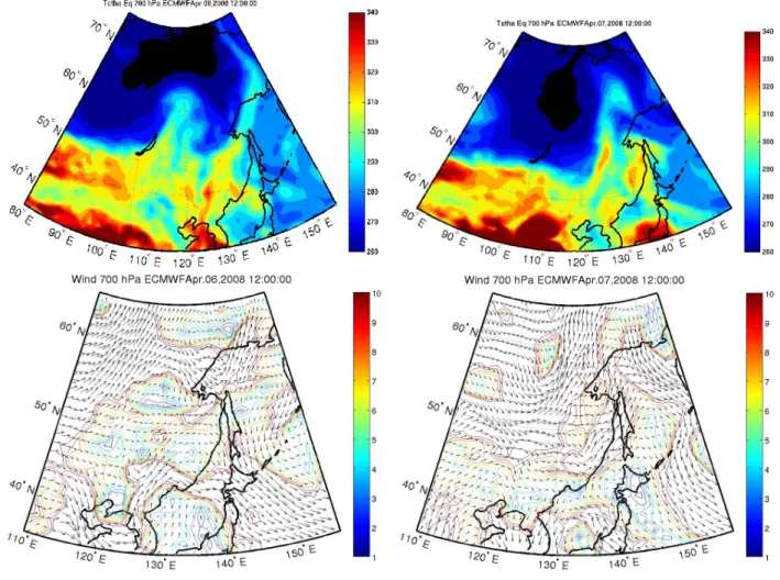
Fig. 10. ECMWF 700 hPa equivalent potential temperature in K (top row) and ECMWF 700 hPa wind field (bottom row) for the 06/04/2008
(left column) and 07/04/2008 (right column) at 12:00 UT. Colored isolines are wind speed in m s−1.
3.2 Air mass origins and CALIPSO overpasses
The cross-section in Fig. 8 nicely shows that the measure-ment area between 3.5 and 5 km in the southern section (<70◦N) is mainly related to European emissions with a fraction of particles larger than 30% coming from the Euro-pean PBL. The area corresponding to the largest lidar sig-nal comes from central Europe with a significant upward motion from the PBL (altitude <2 km) to the 4 km altitude range above Denmark (Fig. 9a). This took place over 3.5 days because of the combined influence of two Low pres-sure systems: one over the North Sea and the other one over the Western Mediterranean sea. Central European emissions first transported by the cold conveyor belt of the southern-most low were then further uplifted in the warm conveyor belt of the northernmost Low.
The aerosol layer observed in the northern section of the flight was transported from Asia as shown by the cross-section of the Asian fraction where boxes with fraction larger than 30% matches exactly the sawtooth motion of the aircraft
between 70.5◦N and 72.5◦N. An example of a trajectory for the box at 72◦N, 3.7 km (Fig. 9b) shows that the upward mo-tion took place in a frontal system developing above North Eastern China from 5 April to 7 April (see the θemap
show-ing the position of the low level front and the advection of warm and humid air mass toward the Arctic in Fig. 10).
The influence of STE below 6 km remains negligible (the PV fraction in the FLEXPART runs are always less than 10%) and the clean region of the lidar section above 3.5 km between 69.5◦N and 70◦N remains influenced by the Eu-ropean emission but uplifting is mainly driven by the April 7 low pressure over the North Sea. The dominant Euro-pean sources are then from the southern coast of the Baltic sea, where lower CO emissions are expected. Aerosols were probably washed out in the northern part of the warm con-veyor belt where heavy precipitation is often encountered at low level (Bethan et al., 1996).
To be more specific about the geographical extent of the Asian and European sources responsible for the aerosol and CO increase, we have also used the map of the potential
Fig. 11. Potential Emission Sensivity (PES) in ns/kg for 4 points of the flight track 68.8◦N–4500 m, 70.2◦N–4200 m, 72◦N–3600 m and 72.4◦N–5250 m. Numbers indicate elapsed time in days since emission along the mean trajectory. (see http://transport.nilu.no/ flexpart-projects?cmp=POLARCAT FRANCE).
emission sensitivity (PES) described in Seibert and Frank (2004) and calculated for different positions along the air-craft track by John Burkhart for the POLARCAT project (web site http://transport.nilu.no/flexpart-projects). The PES is shown in Fig. 11 for 4 different latitudes along the flight cross-section: 68.6◦N (European plume), 70.2◦N, 72◦N, 72.4◦N (Asian plume).The 72.4◦N and 72◦N air masses correspond to respectively the aerosol layer at 5 km and at 3.7 km in the northernmost part of the lidar cross-section. We can see that the European emissions related to our observa-tions are mainly from Eastern Europe and that the air mass lifetime is of the order of 4–5 days. For the Asian plume, we can see that it cannot be regarded as a single layer with a similar history but most likely to two different plumes: one is related to the fire emissions which took place in April 2008 over Siberia (see the 10-day mean fire map plot measured by MODIS from 31/03/2008 to 09/04/2008 in Fig. 12) east of Lake Ba¨ıkal and the other one is related to the anthropogenic emissions from North Eastern Asia (Streets and Waldhoff, 2000). The strong impact of the spring 2008 Siberian fires
on the atmospheric composition have been already observed over Alaska (Warneke et al., 2009) and by the satellite obser-vations (Coheur et al., 2009).
Using air mass trajectory estimates similar to the results shown in Fig. 9, one can look for the CALIPSO satellite tracks coinciding with the transport of these aerosol layers to the region of the aircraft measurements. This was done for three groups of trajectories corresponding to the boxes of Fig. 8 which are within the black rectangles indicated in this figure: (i) the first area near 69◦N (six trajectories) matches the European plume (layer I in the lidar data), (ii) the sec-ond one at 4 km near 70.5◦N (six trajectories) matches the
southern part of the Asian plume (layer II-A) and (iii) the last rectangle at 4 km near 72◦N (four trajectories) corre-sponds to the northern part of the Asian plume (layer II-B). A CALIPSO track was selected if the time and horizontal po-sition of the satellite overpass was less than, respectively 2 h and 200 km, from the air mass positions in the FLEXPART runs. The track sections (line) and the FLEXPART air mass positions (stars) are shown in Fig. 13 where the color scale
Fig. 12. Fires detected by MODIS over a 10-day period 31/03/2008
to 09/04/2008. Each colored dot indicates a location with at least one fire during the compositing period. Color ranges from low (red) to high (yellow) fire counts.
corresponds to the elapsed time between the CALIPSO ob-servations and the aircraft obob-servations. One can see that the evolution of the aerosol content of the 3 selected groups can be analysed for a 6 day period for the Asian plume and a 4 day period for the European plume, i.e. the time correspond-ing to the transport from the source region. The selected CALIPSO observations are coming from the same source region for group (ii) and (iii) but the pathways are slightly different. The air masses and the corresponding CALIPSO observations remain over the continent with the northward transport near 135◦E three days before for group (iii), i.e. the northern section of the plume. The group (ii) shows a longer pathway with the northward transport more often over the Pacific ocean and even toward Alaska before coming back west to Scandinavia. Several CALIPSO overpasses are in-deed above Alaska for group (ii).
Even though there are different pathways for group (ii) and (iii), we will not distinguish the two groups any fur-ther as their air masses are both connected to the position of the Siberian fires and north-east Asian emissions. The use of CALIPSO to distinguish aerosol layers related to these two sources will have to be deduced from the actual lati-tude/longitude of the detected layers in the CALIPSO ob-servations over Asia.
Notice that there is a likely Lagrangian connection be-tween aircraft observations made in Alaska bebe-tween 4 and 7 April and the lidar observations of group (ii). This will be studied in a future paper using a Lagrangian model for aerosol aging.
4 Optical properties of the aerosol plumes using CALIOP
The level-2.1 version 2.01 CALIOP aerosol data products have been analysed along the selected CALIPSO track us-ing the 5-km horizontal average profiles (Liu et al., 2009).
Fig. 13. Calipso track sections (line) and FLEXPART air mass
posi-tions (*) along FLEXPART trajectories initialized in the black rect-angles of Fig. 8 (top left panel for 69 5◦N, top right and bottom panel for respectively the 70.5◦N and 72◦N rectangles). The col-ors scale indicates the elapsed time in hour between the CALIPSO observation and the aircraft observation.
Table 3a. Aerosol layer characteristics from the CALIPSO observations for the backward FLEXPART model run initialized at 69.5◦N– 72.5◦N, 3.5–4.5 km (Layer II-A and II-B). Lines are colored to indicate Siberian fires (light brown), mixed Asian sources south of 52N (gold and red to indicate when dust are expected to influence the mixture) from trajectory analysis.
CALIOP Flexpart Mean Pseudo Pseudo Aerosol FCF
Date Time Start End layer β532 Color Mean Color
UT Lat./Lon Lat./Lon alt, km km−1sr−1 ratio δ532 ratio
05/04 03:21 51.3/135.8 52.4/135.4 5.2-7.2 22±4.10−4 0.36±0.16 0.12±0.17 0.54±0.51 D 05/04 05:00 51.73/110.94 52.38/110.63 2.2–4.2 18±3.10−4 0.33±0.16 0.10±0.11 05/04 12:28 61.81/−146.33 63.65/−144.88 2.1–4.1 39±22.10−4 0.38±0.45 0.11±0.15 05/04 17:25 42.55/130.16 47.77/132.06 1–2.2 39±12.10−4 0.39±0.18 0.07±0.06 0.55±0.71 P.D. 05/04 19:04 56.34/111.3 61.41/114.49 3.7–5.7 14±3.10−4 0.27±0.19 0.04±0.04 0.72±1.28 P.D. 05/04 20:43 56.26/86.54 57.09/87 3.2–5.2 16±3.10−4 0.3±0.14 0.06±0.04 0.7±0.87 P.D. 05/04 22:21 59.06/63.46 62.42/65.8 5.3–7.3 12±2.10−4 0.32±0.15 0.09±0.05 05/04 22:21 68.55/71.74 69.83/73.41 5.5–7.5 13±3.10−4 0.26±0.17 0.11±0.06 06/04 04:05 50.26/125.48 51.4/124.98 1.5–3.5 25±3.10−4 0.33±0.16 0.06±0.11 0.58±0.52 P.D. 06/04 07:22 56.41/73.06 57.06/72.7 5–7 15±2.10−4 0.3±0.17 0.11±0.11 0.59±0.65 D 06/04 13:12 65.12/−154.4 67.1/-152.42 3.7–6.5 15±5.10−4 0.05±0.4 0.07±0.07 06/04 14:50 65.59/−178.68 65.72/-178.56 4.8–6.8 15±3.10−4 0.53±0.35 0.10±0.08 06/04 19:47 57.97/101.42 58.62/101.81 4.7–6.7 10±1.10−4 0.13±0.1 0.04±0.02 0.54±1.2 D 06/04 23:51 58.61/−175.44 59.43/-175.96 4.9–6.9 21±4.10−4 0.22±0.18 0.09±0.11 07/04 03:09 47.42/140.54 50.5/139.28 1-3.4 40±12.10−4 0.55±0.18 0.13±0.18 0.76±0.82 D 07/04 03:09 50.81/139.14 51.78/138.71 1-2.8 35±12.10−4 1.02±0.61 0.11±0.17 1.59±2.39 D 07/04 04:48 52.78/113.53 53.26/113.3 2.7–4.7 32±7.10−4 0.33±0.14 0.00±0.08 0.47±0.48 S 07/04 16:20 72.81/155.56 73.83/157.66 4.7–7 13±2.10−4 0.27±0.13 0.02±0.02 07/04 17:13 52.04/136.95 56.15/139.01 1–3.3 27±6.10−4 0.31±0.25 0.04±0.03 07/04 17:13 59.11/140.74 64.18/144.49 1–3.4 27±8.10−4 0.31±0.15 0.02±0.03 07/04 17:59 75.09/136.02 76.98/141.93 5–7.3 13±2.10−4 0.27±0.14 0.03±0.04 07/04 18:52 58.94/115.92 59.59/116.33 5–7 11±1.10−4 0.24±0.13 0.07±0.04 0.88±1.06 D 08/04 00:35 76.26/150 76.8/148.18 5–7.4 17±4.10−4 0.27±0.2 0.16±0.11 08/04 02:14 61.95/146.76 63.27/145.72 1–3 25±4.10−4 0.3±0.1 0.04±0.11 08/04 17:56 59.82/130.39 64.89/134.3 2.1–6.6 17±3.10−4 0.25±0.14 0.04±0.03 08/04 20:21 80.38/126.27 80.71/129.88 4.8–7.4 13±2.10−4 0.28±0.13 0.00±0.08 08/04 22:00 81.3/113.75 81.52/118.4 4.8–7.4 15±2.10−4 0.3±0.14 0.03±0.09 D: Dust. C.C.: Clean Continental. P.D.: Polluted Dust. S: Smoke.
We have considered the aerosol layer properties when the aerosol layer altitude is less than 1 km away from the air mass altitudes calculated by FLEXPART. Two additional condi-tions are: a minimum horizontal averaging of 80 km and a 3% minimum threshold value for the layer optical depth at 532 nm to be faithfully analyzed. The last two conditions are necessary considering the small aerosol optical depths of the layers revealed by the airborne lidar observations. For a given CALIPSO track, the average position of all the nearby FLEXPART air masses is calculated and the track is analysed over a ±300 km distance around this average position. The mean 532-nm attenuated backscatter, the pseudo color ratio between 1064 and 532 nm and the 532-nm volume depolar-ization ratio are reported for all the layers which fullfilled the previous conditions in Tables 3a and 3b for the FLEXPART trajectories of group (ii) and (iii) and in Table 4 for the group
(i). The comparison between the CALIPSO tracks in Fig. 13 and the time and position of the detected layers show that 65% and 50% of the CALIOP data exhibit aerosol layers with optical depths >0.03 for the Asian plumes (Table 3a, 3b) and the European plume (Table 4) respectively. We can notice that the uncertainties in the color ratio and the depolariza-tion ratio are often very large and cannot be used for a truly quantitative analysis of the aerosol composition and evolu-tion. The largest possible ratios (i.e. the mean+the standard deviation) still contain a meaningful indication about the pos-sible source and the rough evolution of the optical properties (see Omar et al. (2009) for interpretation of the color ratio and the depolarization ratio for aerosol classification). The Cloud Aerosol Discrimination (CAD) score have been calcu-lated for the aerosol layers listed in Tables 3a, 3b, 4. They are always larger than 50% and 3/4 of the CAD values are even
Table 3b. continue from Table 3a, layers in the area where the aircraft flew are indicated in green.
CALIOP Flexpart Mean Pseudo Pseudo Aerosol FCF Date Time Start End layer β532 Color Mean Color
UT Lat./Lon Lat./Lon alt, km km−1sr−1 ratio δ532 ratio
09/04 02:57 67.82/130.51 68.44/129.77 4–6.9 21±5.10−4 0.5±0.19 0.08±0.20 09/04 17:47 71.9/132.25 75.98/141.63 3.8–5.8 21±6.10−4 0.29±0.12 0.03±0.03 09/04 19:26 78.32/126.06 80.65/143.1 3–6.3 16±2.10−4 0.32±0.12 0.03±0.07 09/04 21:05 80.89/121.22 81.16/125.21 4.1–6.1 14±2.10−4 0.35±0.18 0.00±0.06 10/04 02:02 77.56/23.72 79.66/35.26 4.6–7.4 14±2.10−4 0.26±0.15 0.03±0.07 0.55±0.65 C.C. 10/04 03:40 81.71/39.83 81.81/47.08 3.7–7.4 20±4.10−4 0.68±0.36 0.03±0.12 10/04 05:19 81.8/20.22 81.82/24.04 3.7–6.7 17±2.10−4 0.15±0.09 0.03±0.09 0.25±0.3 C.C. 10/04 06:58 81.32/19.38 81.68/10.17 3.7–7.4 15±2.10−4 0.25±0.17 0.05±0.11 0.46±0.56 C.C. 11/04 02:45 73.66/1.25 75.67/6.29 3–5.6 16±2.10−4 0.27±0.12 0.02±0.03 0.62±0.62 S D: Dust. C.C.: Clean Continental. P.D.: Polluted Dust. S: Smoke.
larger than 75% for the layers discussed in this work. This is a good indication that the features detected by CALIOP are indeed aerosol layers (Eguchi et al., 2009).
Like for the airborne lidar analysis, the aerosol color ratio is also reported in Tables 3a, 3b, 4. The error on this ratio is larger than the error on the pseudo ratio, with values ranging between 100% and 200%. This ratio varies between 0.25 and 0.7 for the smallest error (100%), and is close to 0.5 on average for layers identified in Table 3a. It is larger than the airborne lidar values of 0.2 reported in Table 2.
We however have to consider attenuation above the air-craft to more directly compare both values. Assuming clean air, considering 5 km as an average altitude flight, and ne-glecting molecular scattering at 1064 nm leads to a overesti-mation of about 15% of space values with respect to aircraft ones. Including upper level aerosols would lead to an ad-ditional increase of the same order, which would make the corrected color ratio derived from space measurements to be about 0.35. This is also the same correction for the com-parison of the pseudo color ratios. This appears acceptable due to the large error bar (mostly linked to calibration error) on this quantity, but also because CALIOP can hardly detect layers with small optical depths (>0.03) and Angstrom co-efficient larger than 2. The CALIOP aerosol color ratio are more comparable to the work of Cattrall et al. (2005) near the Asian sources where there are backscatter ratio (R >3) and where the aerosol color ratio are of the order of 0.6–0.7 (see layers colored in gold Table 3a and discussion hereafter on source attribution). This is consistent with a mixture of pollution (color ratio of 0.5) and dust aerosol (color ratio of 1).
The analysis of the two tables shows that the CALIOP lay-ers detected in the region 65–85◦N, 10–30◦E (i.e. in the vicinity of the aircraft measurement zone and colored in green in table 3b exhibit moderate 532-nm backscatter values (1.4–1.7 10−3km−1sr−1, i.e. a backscatter ratio R between
1.6–1.9), low color ratio (≤0.25) and almost no depolariza-tion (≈3%). This is consistent with the properties of the lay-ers measured by the aircraft (Table 2). The depolarization values measured at 355 nm by the aircraft (2%) are slightly smaller than the expected δ355 (2.5%) for a δ532 of 3%, but
the CALIOP volume depolarization values in this region are nevertheless smaller than all the CALIOP data reported in Tables 3a and 3b. The good correspondence between the aerosol properties of the CALIOP layers and the airborne lidar layers for a time scale of 1 day, is the first necessary condition if one aims at using the CALIOP observations fur-ther upwind in order to unsderstand the sources of the aerosol layers seen by the aircraft.
The analysis of Table 3a and 3b focused on layers with backscatter values, β532≥2 10−3km−1sr−1(R ≥ 2) i.e. with
an intensity strong enough to be able to discuss the optical properties. The position of the layers must also be considered in the interpretation of this table as three Asian sources are known to dominate the aerosol composition at this time of the year: the desert dust advected from the Gobi and Taklamakan desert (Duce et al., 1980) in the latitude band 40◦N–50◦N, the industrial emissions from the Heilongjiang region further east in the same latitude band, and the forest fires from the Lake Baikal region in the latitude band 50◦N–55◦N. There-fore four main results can be underlined from this table:
– Looking at the strongest aerosol layers prior to April 8, two kinds of aerosol properties can be found in the 45◦–52◦N where several sources influence the aerosol properties (layers colored in gold in table 3a): one with low pseudo color ratio (near 0.3) and low δ532 (0–7%)
for longitude <125◦E (text in black Table 3a), and the other one with larger pseudo color ratio (0.5 to 1) and larger δ532(10–14%) for longitude > 135◦E (i.e. near
Table 4. Aerosol layer characteristics from the CALIPSO observations for the backward FLEXPART model run initialized at 68.5◦N–69◦N, 3.5–5 km (Layer I).
CALIOP Flexpart Mean Pseudo Pseudo Aerosol FCF Date Time Start End layer β532 Color Mean Color
UT Lat./Lon Lat./Lon alt, km km−1sr−1 ratio δ532 ratio
08/4 01:27 52.05/13.36 55.86/15.24 1.7–5.4 27±1.10−4 0.44±0.28 0.08±0.06 0.7±0.54 D 09/4 02:11 58.45/5.91 62.72/8.87 3.1–5.3 17±4.10−4 0.23±0.21 0.05±0.06 0.47±0.91 C.C. 10/4 02:54 66.26/1.21 70.21/5.97 2.5–5.3 16±4.10−4 0.23±0.18 0.04±0.03 0.51±0.97 P.D. 10/4 10:16 64.76/23.94 64.88/23.82 2.6–5.0 39±13.10−4 0.40±0.50 0.10±0.14 0.53±1.13 P.D. 11/4 01:58 65.94/14.79 68.41/17.49 2.7–5.2 16±3.10−4 0.10±0.17 0.03±0.02 0.18±0.71 C.C. D: Dust. C.C.: Clean Continental. P.D.: Polluted Dust. S: Smoke.
– Near the Siberian fire sources (55◦–60◦N, 90◦–120◦E),
β532≤2 10−3km−1sr−1 (R ≈ 1.5) with a 0.3 pseudo
color ratio and a weak δ532(4–7%), i.e. with probably
small aerosol which did not have time to grow as when transported through a very humid frontal system (layers colored in light brown in Table 3a)
– At latitude larger than 60◦N (i.e. in the Arctic region), one can distinguish two regions: (i) the layers detected above Alaska with a color ratio of 0.3–0.4 and some de-polarization (9–10%) although smaller than the values for lower latitudes near the Asian Pacific coast, (ii) the layers in the Eurasian Arctic with a variable color ratio 0.3–0.5 and lower δ532(2–8%)
– As the air masses are transported from Asia to Scandi-navia across the Arctic, there is a general tendency for decreasing β532 from 3 to 1.5 10−3km−1sr−1 (i.e. R
from 3 to 1.7) and fewer air masses with elevated pseudo color ratio or pseudo depolarization ratio. Notice also that there is not a very clear dependency of the optical properties with altitude in the detected layers considered in this study.
The CALIOP aerosol feature classification flag (FCF) de-rived from the operational products is also reported in Ta-bles 3a, 3b, 4. This classication is mainly based on the de-polarization and color ratio, the attenuated backscatter am-plitude and layer altitude (Liu et al., 2004) . This can be compared with our own interpretation of the aerosol source influencing the layers. One can see that the agreement is certainly good for the layers where we suspect the desert dust to be mixed with the polluted emissions from north-east Asia (gold). The main discrepancies are for the layers in the Siberian fire region where the CALIOP operational products assumed mainly dust sources, while our analysis suggest a dominant influence from boreal fires. The CALIOP analysis is mainly related to the weak increase of δ532, but it does not
take into account the likely small size of the aerosols and the
large number of fires in this region in April 2008. Also the CALIOP FCF tends to define layers encountered after sev-eral days of transport as clean continental, while our analy-sis shows a connection between the Asian polluted sources and the area above Scandinavia. This is probably a limit of the CALIOP FCF for making a precise continental source at-tribution after several days of transport which resulted on a large decrease of the attenuated backscatter.
One plausible hypothesis for explaining the largest δ532
and elevated pseudo color ratio for the CALIPSO layers in the area (45◦–52◦N, 135◦–140◦E) is that the southernmost CALIPSO tracks near the coast are influenced both by the desert dust and north-east Asian emissions. The higher color ratio is consistent with larger aerosol particles resulting from a remaining influence of dust but also from the likely growth of the pollution aerosol in the frontal system responsible for the northward transport which develops near the Pacific coast on 5–7 April (Fig. 10). Airborne in-situ aerosol measure-ments of the ratio of ultrafine (3–70 nm) to fine particles (70– 200 nm) over Siberia in Spring 2006 by Paris et al. (2009) have shown, for similar meteorological conditions, that this ratio decreases for polluted air masses from north-east Asia. Further west, where northward motion is less efficient, the Siberian boreal fires gradually become the main aerosol source (Warneke et al., 2009), explaining a significant de-crease in both the pseudo color ratio and δ532, as expected
for biomass burning aerosol according to the work of Cat-trall et al. (2005). This means that the three sources have in-fluenced the aerosol composition over Scandinavia and that the depolarization ratio should provide a way to separate the biomass burning plume from the north-east Asian emissions because of the remaining influence of the desert emissions in the 40◦N–50◦N latitude band.
Above 60◦N, the Alaskan layers can be considered as aged Asian layers being transported across the Pacific to Alaska as reported in the analysis of the 2008 spring pe-riod transport pathways described in Fuelberg et al. (2009), but also from the modeling work of Fisher et al. (2009)
showing the widespread influence Asian CO sources includ-ing Alaska. This can explain the values of the depolariza-tion ratio which are intermediate between the low values above Scandinavia and the large values above North East-ern Asia. Considering all the layers in the Arctic region the slight decrease of the color ratio which is concomitant with the lower β532, would indicate the gradual removal of the
largest aerosol particles due either to mixing of the different aerosol type being present above Asia or to the wet removal of the largest hydrophilic aerosol particles during the trans-port processes.
Finally the CALIPSO analysis of the aerosol layer prop-erties above Asia would now suggest that the source attri-bution of the different layers observed by the lidar in the Asian plume could be the following: remaining influence of north-east Asian emissions mixed with dust for the layer II-A at 69.7◦N and more predominantly Siberian fire
influ-ence for the layer II-B further north. The combined use of FLEXPART together with analysis of the CALIPSO data al-lows more robust conclusions to made regarding the different sources influencing observed aerosol layers north of Scandi-navia after more than 5 days of transport from source regions. When it is compared with the analysis of the Asian plume, the results of Table 4 show smaller changes of the aerosol properties during the transport from central Europe. The pseudo color ratio and the depolarization ratio are less than 0.4 and 8%, respectively, above the sources in central Eu-rope. These values are intermediate between the ones ob-served for the two types of Asian layers discussed previ-ously . This is not so surprising since industrial European emissions dominate the aerosol composition where larger aerosols from the accumulation modes are less numerous. Episodic transport from the Sahara in the exported air mass from Europe is possible (Hamonou et al., 1999), Fuelberg et al. (2009) showed that 10-day trajectories reaching 70◦N and originating from Sahara were almost negligible during the 2008 spring season compared to the potential export of Asian dust.
5 Conclusions
In this paper we have analysed airborne and spaceborne lidar aerosol data related to the transport of two different sources into the Arctic during April 2008: a European plume and an Asian plume. In the case studied here both plumes ex-hibit elevated CO concentrations indicating a significant frac-tion of either biomass burning or anthropogenic pollufrac-tion sources. Although the aerosol optical depths are similar for both layers, their optical properties are quite different. We used mainly the pseudo volume depolarization at 355 nm and pseudo color ratio between 1064 and 532 to distinguish both layers because they are more stable quantities when look-ing at relative variations of the optical properties of layers with low aerosol optical depths (<4%), as encountered in this
study. These ratios are also more comparable to CALIOP version 2.1 aerosol layer properties than other parameters, e.g. the aerosol color ratio or the aerosol depolarization ratio. The European plume (layer I) contains smaller particles with very low 355 nm depolarization (1.6±0.3%) and low pseudo color ratios (0.009±0.002%). The Asian plume is characterized by larger particles and some 355nm depolar-ization (2.1±0.3%) in one layer (layer II-A, i.e. with a larger fraction of dust particles). Measurements of the aerosol size spectrum along the flight have also shown that the variability of the pseudo color ratio can be related to the actual change of the aerosol size distribution even for layers where the opti-cal depth is small and consequently an increase of the pseudo color ratio error. This also gives confidence in the possibility of using the same kind of information in the CALIOP aerosol data products (pseudo color ratio between 1064 and 532 nm, pseudo volume depolarization at 532 nm). in the analysis of aerosol layers of moderate intensity when transported across the Arctic, even considering the expected larger error bar (30–100%) in the CALIOP data compared to the errors in the aircraft observations.
The comparison of the CALIOP data with the airborne data over northern Scandinavia showed that the pseudo color ratio and the volume depolarization ratio are in a reasonable agreement considering the error bar on the CALIOP data and the fact that time and spatial coincidences of the measure-ments are only possible in a 1-day time frame and a 500 km by 800 km longitude/latitude band. Nevertheless, these re-sults show that CALIOP aerosol data products can be used to study the evolution of layer aerosol properties over a period of several days.
To understand the variability of the airborne observations, the transport of the air masses was investigated using spe-cific FLEXPART simulations including calculation of the PBL air fraction originating from three different mid-latitude source regions: Asia, North America and Europe. Results from the transport model were combined with the CALIPSO overpasses to link our observations with CALIOP results ob-tained near the remote sources (Asia, Central Europe), con-sequently improving the identification of the aerosol sources responsible for the aerosol layers observed by the aircraft af-ter a transport time of more than 4–5 days.
For example, above Asia, the CALIOP data indeed sug-gest more 532 nm pseudo depolarization (up to 15%) and the largest pseudo color ratio (>0.5) for north-east Asian emissions where there is a mixture of Asian pollution and dust, while low depolarization together with smaller and quasi constant pseudo color ratio (≈0.3) are observed for the Siberian biomass burning emissions. A similar difference is visible between layer II-A and II-B observed by the aircraft above Scandinavia. It means that distinct signatures of the three aerosol sources (biomass burning, industrial emissions and desert) are still visible after being transported across the Arctic with the influence of the mixture of Asian pollution and dust being stronger for layer II-A. Of course the analysis
remains qualitative considering the difficulty in quantify-ing the different processes modifyquantify-ing the aerosol proper-ties. This would require specific Lagrangian modeling of the aerosol evolution which is not within the scope of this paper. Notice however that it would have been difficult to discuss the remaining influence of different aerosol sources using the trajectory model alone which is less able to distin-guish source regions after several days of transport.
The analysis of the time evolution of the aerosol optical properties revealed by CALIOP between the source regions and northern Scandinavia after 4–5 days of transport over the Arctic, suggests a gradual decrease in the 532-nm attenuated backscatter, the volume depolarization ratio and the pseudo color ratio which can be related to the removal of the largest particles in the accumulation mode (e.g. by wet removal in the frontal system responsible for the northward transport). A mixture of the three Asian aerosol sources also contributes to reductions in the volume depolarization and pseudo color ratio towards their lowest values, respectively 2% and 0.1.
The analysis of the European plume showed aerosol opti-cal properties intermediate between the two Asian sources with pseudo color ratios never exceeding 0.4 and moder-ate volume depolarization ratios being always less than 8%, i.e. less aerosol from the accumulation mode. In common with the Asian plume, the time evolution of the European plume suggests the removal of the largest particles, thus ex-plaining the aerosol spectrum observed by the aircraft in this case.
Finally, one conclusion of this paper is that CALIOP aerosol products have indeed a large error bar when dealing with quantities like the pseudo color and volume depolar-ization ratio, but are however valuable tools making source attribution of aerosol layers when used in conjunction with a Lagrangian transport model. It works also for aerosol lay-ers of moderate intensity far away from the major aerosol sources. The comparison with the CALIOP operational FCF aerosol classification indeed show a good agreement for dust source identification, but also differences with our analysis where we include more information (air mass transport, po-sitions of forest fires back in time, pseudo color ratio) than the CALIOP methodology based on the depolarization ratio, the local surface type and the attenuated backscatter inten-sity.
Appendix A
Backscatter lidar parameter definition
In this appendix, we are aiming at defining the parame-ters derived from a backscatter lidar and more precisely from the knowledged of the total volume backscatter coef-ficient at wavelength λ which can be split into the molecular (Rayleigh) and aerosol contribution:
βλ(z) = βλ,m(z) + βλ,a(z) (A1)
where the subscripts m and a specify, respectively, molec-ular, and aerosol contributions to the scattering process. A backscatter lidar measures the range corrected lidar signal,
Pλ(z), at range z, which can be related to βλ(z)by the
fol-lowing equation:
Pλ(z) = Kλ(βλ,m(z) + βλ,a(z)).Tλ,m(z)2.Tλ,a(z)2. (A2)
where Kλthe range independent calibration coefficient of the
lidar system and T2is the two-way transmittance due to any scattering (or absorbing) species along the optical path be-tween the scattering volume at range z and the lidar. The two-way transmittance for any constituent, x, is
Tx(z)2=exp(−2τx(z)) = exp(−2
Z z
0
σx(z0)dz0). (A3)
where τx(z)specifies the optical depth and σx(z)is the
vol-ume extinction coefficient. Molecular contribution can be estimated with a good accuracy using either a density model or meteorological radiosonde data available for the measure-ment area. When the aerosol contribution is negligible at a range z0near the lidar (i.e. where τx(z0)is small), one can
determinate the lidar system constant K from the value of
P (z0). If we divide P (z) by this value and normalize to the
Rayleigh contribution, we obtain the attenuated backscatter ratio, R(z), given by:
R(z) = P (z)
Kβλ,m(z).exp(−2τλ,m(z))
≈1 +βλ,a(z)
βλ,m(z)
(A4) if τλ,aremains small (this is the case for this study).
When a linear polarized laser beam is emitted, depolar-ization related to backscattering in the atmosphere can be measured by a receiving lidar system with an optical selec-tion of the parallel- and cross-polarized signal.The backscat-ter ratios, R, for perpendicular- and parallel-polarized light are defined as R⊥(z) =1 + β⊥,a(z) β⊥,m(z) Rk(z) =1 + βk,a(z) βk,m(z) (A5) and the ratio of the aerosol cross- to parallel-polarized backscatter coefficient is called the linear volume depolar-ization ratio, δa, given by:
δa(z) = β⊥,a(z) βk,a(z) =R⊥(z) −1 Rk(z) −1 .δm δm= β⊥,m βk,m (A6) The Rayleigh depolarization and its wavelength dependency can be found in Bucholtz (1995), e.g. δm=0.015 at 355 nm.
Since this ratio depends critically on the absolute accuracy of the backscatter ratio retrieval, the ratio of the total cross-to the cross-total parallel-polarized backscatter coefficient is also used and called hereafter the pseudo depolarization ratio δ given by: δ(z) =β⊥(z) βk(z) =R⊥(z) Rk(z) =δa(z)(1 − 1 Rk(z) ) + δm Rk(z) . (A7)
The pseudo depolarization ratio, δ, tends to δmonly in a clean
region where Rk tends to 1. Notice that in a thick aerosol
layer where the aerosol depolarization is less than the molec-ular depolarization, δ could tend to zero. The pseudo de-polarization ratio δ has the advantage of being less unstable when the aerosol layer is weak and it is also less dependent on instrumental parameters (Cairo et al., 1999). According to Freudenthaler et al. (2009), the aerosol depolarization ra-tio δahas only a small spectral variation between 532 nm and
355 nm for dust particles, i.e. for aerosol with a large depo-larization value. For example, they found that δa is 0.3 at
532 nm and 0.28 at 355 nm for saharan dust plume. However the wavelength dependency of δ is related also to the spec-tral change of the backscatter ratio. This will have to taken into account when comparing δ355and δ532. For example, the
layer II-A discussed in this paper has a δavalue of the order
of 3%, while R355=1.5 and R532=2. Assuming no spectral
variation of δaimplies a δ variation from 2% to 2.2% when
switching the wavelength from 355 to 532 nm.
The ratio of aerosol backscatter at 1064 nm to the aerosol backscatter at 532 nm is called the color ratio, CR, given by CR(z) =βa,1.06(z) βa,0.53(z) =R1.06(z) −1 R0.53(z) −1 . 1 16 (A8)
where 1/16 is the ratio of the 1064-nm to the 532-nm molec-ular backscatter. The ratio of total backscatter at 532 nm and the total backscatter at 1064 nm can also be calculated for the same reasons which lead us to use the pseudo depolarization ratio. This new ratio, called hereafter the pseudo color ratio, is related to CR by the following equation:
CR∗(z) =β1.06(z) β0.53(z) =CR(z)(1− 1 R0.53(z) )+ 1 16R0.53(z) (A9) The pseudo ratio CR* can be as small as 1/16, when the aerosol contribution is small (i.e. R much less than 1.5). The CR ratio provides a better representation of the size influence on the aerosol optical properties variation with the wave-length (O’Neill et al., 2003) as it is more directly related to the Angstr¨om coefficient which is the standard parameter for discussing this spectral dependency and which is defined as:
k = −dlnτa
dlnλ. (A10)
Since k depends on aerosol extinction and not on aerosol backscatter coefficients, the relation between k and CR de-pends on the ratio of these two coefficient, also called the lidar ratio B. The ratio CR is related to k by the equation: CR(z) = B0.5,a(z)
B1.06,a(z)
.2−k. (A11)
When the fine mode aerosol contribution decreases, k varies from values around 2 to values near 0 and CR increases from values near 0.5 to values near 1, assuming that the corre-sponding B0.53,a
B1.06,a changes goes from 2 to 1 according to
Cat-trall et al. (2005). The change of the pseudo ratio CR* goes
in the same direction, but with a smaller amplitude as R de-creases. For example, CR* does not exceeds 0.5 even for the largest CR values when R remains around 2. Notice also that for small optical depths and small values of the coarse mode fraction, the model calculation of (O’Neill et al., 2003) suggests that k can be larger than 2 and therefore the small-est CR* may become less than 0.2 even when R does not become too small (i.e. above 1.5).
Acknowledgements. The UMS SAFIRE is acknowledged for
supporting the ATR-42 aircraft deployment and for providing the aircraft meteorological data. The POLARCAT-FRANCE project was supported by ANR, CNES, CNRS/INSU and IPEV. F. Blouzon and D. Bruneau are acknowledged for their contribution to the lidar operation during flights, and Ariane Bazureau for her work on FLEXPART modeling. John Burkhart from NILU is acknowledged for providing FLEXPART products on the POLARCAT web site. The NASA data center in charge of the CALIPSO data is greatfully acknowledged for providing the CALIOP lidar data.
Edited by: A. Stohl
The publication of this article is financed by CNRS-INSU.
References
Atlas, E. L., Ridley, B. A., and Cantrell, C.: The Tropo-spheric Ozone Production about the Spring Equinox (TOPSE) Experiment: Introduction, J. Geophys. Res., 108(D4), 8353, doi:10.1029/2002JD003172, 2003.
Bethan, S., Vaughan, G., and Reid, S.: A comparison of ozone and thermal tropopause heights and the impact of tropopause defini-tion on quantifying the ozone content of the troposphere, Q. J. Roy. Meteorol. Soc., 122, 929–944, 1996.
Browell, E. V., Hair, J., Butler, C., Grant, W., DeYoung, R., Fenn, M., Brackett, V., Clayton, M., Brasseur, L., Harper, D., Rid-ley, B., Klonecki, A., Hess, P., Emmons, L., Tie, X., Atlas, E., Cantrell, C., Wimmers, A., Blake, D., Coffey, M., Hannigan, J., Dibb, J., Talbot, R., Flocke, F., Weinheimer, A., Fried, A., Wert, B., Snow, J., and Lefer, B.: Ozone, aerosol, potential vor-ticity, and trace gas trends observed at high-latitudes over North America from February to May 2000, J. Geophys. Res., 108(D4), 8369, doi:10.1029/2001JD001390, 2003.
Bucholtz, A.: Rayleigh-scattering calculations for the terres-trial atmosphere, Appl. Opt., 34, 2765–2773, doi:10.1364/AO. 34.002765, http://ao.osa.org/abstract.cfm?URI=ao-34-15-2765, 1995.
Cairo, F., Donfrancesco, G. D., Adriani, A., Pulvirenti, L., and Fierli, F.: Comparison of Various Linear Depolarization Pa-rameters Measured by Lidar, Appl. Opt., 38, 4425–4432, http: //ao.osa.org/abstract.cfm?URI=ao-38-21-4425, 1999.